Chapter 8

DRIVING IN THE CITY

 

 

As noted in the previous chapter, in many very large cities a car is not needed at all. But there also are many cities and towns where it is essential to have a vehicle. One advantage of driving over public transportation can be that one does not have to keep stopping at intermediate locations on the way to one’s destination (traffic permitting). Of course, the daily commute can be extremely frustrating when it is of the stop-and-start variety, and the gas consumption becomes prohibitive. At the time of writing the price of petrol in the UK is far higher (by a factor of two) than the equivalent cost of gas in the U.S. It must be the different spelling that causes this. But before discussing that and other driving-related topics, let’s start with an unrealistic but amusing and informative question.

X = : GASOLINE CONSUMPTION IN THE CITY

Question: A car travels from a home in the suburbs to a downtown office building, somehow maintaining a constant speed of 30 mph. On the return journey it maintains a constant speed of 60 mph. What is its average speed?

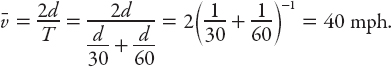
No, it’s not 45 mph, sorry. The car spends twice as long traveling at 30 mph as it does returning at 60 mph, so the average speed will be “weighted” toward the lower speed. The correct answer is 40 mph. To see why, the average speed is defined as the total distance traveled divided by the total time (T) for the round trip. For those who are concerned that we have not specified the distance from the proverbial “A to B”—not to worry, let’s just call it d. Then the average speed is

In fact, the above result is the harmonic mean of the two speeds. The harmonic mean of a set of numbers is the reciprocal of the arithmetic mean of the reciprocals! Put more obviously in mathematical terms, for a set of n numbers x_i, i = 1, 2, 3, . . . n, the harmonic mean H is

That’s the power of algebra for you! The incorrect answer of 45 mph is based on the arithmetic mean, which as we see, is not the appropriate measure of “average” for this problem. This difference is exacerbated by considering more than one “vehicle”; suppose that nine vehicles traverse a route one mile in length, and that all travel at the posted speed limit of 55 mph. I decide to walk the route at a reasonable pace, say 4 mph. The average speed for all ten trips, as computed by using the arithmetic mean is

On the other hand, if we calculate the total distance traveled and divide it by the total time taken, the result is

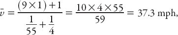
a considerable difference.

Question: If we replace “speed” by “average speed” in the above question, does it change the result?

Exercise: Generalize the first result for speeds v₁ and v₂.

X = ΔE: Question: How does gasoline consumption vary with speed?

In recent years, as well as several decades ago, the increasing costs of oil and gasoline have threatened to change the habits of American motorists, and in some cases has done so (albeit for a limited period of time, after which gas prices have declined, and everything reverts to the status quo). We know that at low speeds in low gears fuel consumption rate is relatively high because of lower efficiency in converting chemical energy to kinetic energy at these speeds. At high speeds the effects of air resistance (or drag) also increases the rate of fuel consumption. So it’s certainly reasonable to conclude that there is an optimal speed (or range of speeds) for which the rate of fuel consumption is minimized.

The national 55-mph speed limit in the U.S. is no longer in existence, but in 1982 a newspaper article stated that one should “Observe the 55-mile-an-hour national highway speed limit.” Furthermore, it stated that “For every five miles an hour over 50, there is a loss of one mile to the gallon. Insisting that drivers stay at the 55-mile-an-hour mark has cut fuel consumption 12 percent for [Company name] of Jacksonville, Florida—a savings of 631,000 gallons of fuel a year. The most fuel-efficient range for driving generally is considered to be between 35 and 45 miles an hour” (“Boost Fuel Economy,” Monterey Peninsula Herald, May 16, 1982, as quoted in Giordano et al. 2003).

My first reaction on reading this was to wonder if the article is referring to fuel consumption for domestic as opposed to commercial vehicles, or both (which seems unlikely). And I very much doubt that the mpg losses are a linear function of speed above 55 mph as suggested. Surely there are more factors that affect how many miles per gallon we get from our vehicles, such as the age of the engine (and maybe the driver!), the type of fuel used, the air temperature, the speed of travel, and the resistive forces of drag and road friction. Drag will depend on the speed and shape of the vehicle and the prevailing atmospheric conditions at the ground (wind in particular). Friction will depend on the condition of the tires, and the type and weight of the car. The nature of the terrain is very important also: is it a flat, smooth road or an unpaved track in a hilly or mountainous region? How good is the driver? Does he drive smoothly where possible, or speed up/slow down in an irregular pattern, even if the road conditions do not warrant it? Is she an experienced driver or a novice? These and probably several other considerations all have bearing on the problem of interest here.

A quick and dirty method

The drag force on most everyday objects is proportional to their cross-sectional area A and the square of their speed v. Therefore driving at highway speeds for a distance d will consume energy E ∝ Av²d. For a given value of d and a small change in v(Δv), the corresponding percentage change in energy expended is [16]

While the change from driving at 70 mph (as many do) to 60 mph (about 14%) may not be considered “small,” we’ll use it anyway, and conclude that there is a nearly 30% drop in fuel consumption. This makes a lot of sense!

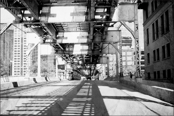
X = d₀: TRAFFIC SIGNALS IN THE CITY

What thoughts typically run through your mind as you approach a traffic signal? Here are some likely ones: will it stay green long enough for me to continue through? Will it turn red in enough time for me to stop? What if it turns yellow and someone is close behind me—should I try to stop or go through? And perhaps related to the latter thought, “Is there a police car in the vicinity?”

Obviously we assume that the car is being driven at or below the legal speed. If the light turns yellow as you approach the signal you have a choice to make: to brake hard enough to stop before the intersection, or to accelerate (or coast) and continue through the intersection legally before the light turns red. Unfortunately, many accidents are caused by drivers misjudging the latter (or going too fast) and running a red light.

The mathematics involved in describing the limits of legal maneuvers is straightforward: integration of Newton’s second law of motion. Suppose that the width of the intersection is s ft and that at the start of the deceleration (or acceleration), time t = 0, and the vehicle is a distance d₀ from the intersection and traveling at speed v₀. If the duration of the yellow light is T seconds, and the maximum acceleration and deceleration are denoted by a₊ and −a₋ respectively, then we have all the initial information we need to find expressions for the two situations above: to stop or continue through. A suitable form of Newton’s second law relates displacement x and acceleration a as

from which follow the speed and displacement equations

We have chosen x(0) = 0. In order to stop before the intersection in at most T seconds, it follows from the second of these equations that

On the other hand, to continue through, we note that the vehicle must travel a distance d₀ + s in less than T, so that requiring x(T) ≥ d₀ + s in the third equation above yields the inequality

In each inequality, we have assumed that the maximum deceleration and acceleration are applied accordingly. Before treating the inequalities graphically, we write them in dimensionless form. This will reduce the number of parameters needed from five to four. To illustrate this, if we divide the distance d₀ by s, we obtain a dimensionless measure of distance in units of s, namely δ = d₀/s. Similarly, we define dimensionless speed by σ = v₀/(s/T), time by τ = t/T, and acceleration by α_± = a_±/(s/T²). Notice that τ is a measure of time in units of the yellow light duration. In these new units, the combined inequalities show that a driver may successfully choose either legal alternative provided that

Now we are in a position to discuss reasonable ranges on these parameters, starting with the physical data. Typical ranges have been taken from the literature [17]. If we adopt the range for the speed approaching the intersection as 10 mph ≤ v₀ ≤ 70 mph (or approximately 15 fps ≤ v₀ ≤ 100 fps), with the bounds 20 ft ≤ d₀ ≤ 600 ft, 30 ft ≤ s ≤ 100 ft, 2 s ≤ T ≤ 6 s, and 3 ft/s² ≤ | a_± | ≤ 10 ft/s², then we find that 0.3 ≤ σ ≤ 16.7, 0.2 ≤ δ ≤ 20, and 0.12 ≤ α_± ≤ 8.3. Since we are measuring time in units of T, the results are relative, even though T itself can and does vary. In Figure 8.1 we plot a generic graph for the bounds on δ(σ) (based on equation (8.6)). There are four regions to consider. The region OAB corresponds to a domain with relatively low speed and small distance, and represents a portion of (σ, δ) space for which either option—stop or continue—is viable. Continuing, the region above ABC is a (theoretically infinite!) region with relatively low speed and large distance, so it is easy to stop before reaching the intersection. BCD is a region with relatively high speed and large distance, and represents a domain in which a violation (or accident) is likely. Finally, below OBD the region corresponds to relatively high speed and small distance, implying it is possible to continue through the intersection before the light turns red.

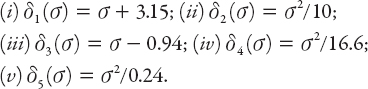
The various δ_i(σ) functions chosen here (with i = 1, 2, 3, 4, also based on equation (8.6)) are defined as follows:

As in Figure 8.1, Figure 8.2 shows dimensionless position/speed graphs identifying regions of safety. Obviously this is a simplistic analysis of the stop-light problem; an experienced and careful driver will have developed some measure of intuition (and caution) concerning whether a successful “continue through” is possible. We have not considered the possibility of skids; they are likely to occur if the deceleration is too large, and poor road conditions (wet, icy, etc.) will greatly affect the required stopping distance. In addressing this problem, Seifert (1962) has suggested posting signs along the roadside indicating a speed at which it is safe to continue through or stop from that location. It’s a thought!

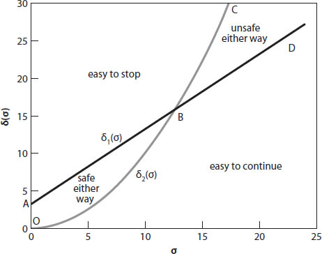
Figure 8.1. Dimensionless distance-speed graphs indicating regions of legal/illegal options based on equation (8.6); δ₁(σ) = σ + 3.15 and δ₂(σ) = σ²/10.

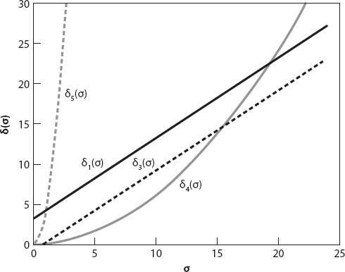
Figure 8.2. Additional dimensionless distance-speed graphs based on equation (8.6) (see Figure 8.1). Here δ₁ is as in Figure 8.1, and δ₃(σ) = σ − 0.94; δ₄(σ) = σ²/16.6; and δ₅(σ) = σ²/0.24.

X = β: AVOIDING ACCIDENTS IN THE CITY

Should the driver of a car try to stop or turn in order to avoid a collision? We shall examine this question for several different situations, the first being when a car approaches a T-intersection with a brick wall directly ahead across the intersection. We shall assume that the junction is free of other vehicles, so the only possibility of collision involves the car hitting the wall. Furthermore, we shall assume that there is no skidding, in which case the coefficient of friction in a turn may be considered to be the same as that in the forward direction. (Skidding would involve the coefficient of sliding friction, in general different from that for rolling friction.)

We can examine three possible choices [18] as illustrated in Figure 8.3: (i) to steer straight ahead and apply the brakes for maximum deceleration; (ii) to turn in a circular arc without braking (using all the available force for centripetal acceleration); or (iii) to choose some combination of (i) or (ii), such as turning first and then steering straight (or vice versa), or even steering in a spiral path. In fact, option (ii) can be ruled out immediately by means of a simple (but nontrivial) argument as follows.

Suppose that the distance of the car from the wall is l and that its speed at that point is v₀. The force required to turn the vehicle (of mass m) in a circular arc of radius l is , but the force required to bring the vehicle to stop in a distance l is . This means that if the car can be turned without hitting the wall, it can be brought to a stop halfway to the wall. Regarding option (iii), a rather more subtle argument [18] shows that the appropriate choice is still to stop in the direction of motion. Apart from a brief discussion below, this will not be elaborated on here; instead we shall examine some other potential driving hazards. It should be no surprise that the worst highway accidents are those involving head-on collisions.

A related problem is this: suppose that we are driving along a road in the right-hand lane for which, at the present speed, our stopping distance is D.

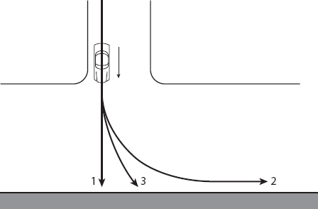
Figure 8.3. The three maneuver options open to the driver.

There is an obstacle ahead—it might be a repair crew, a stalled truck, or even a vehicle moving more slowly than we are (in the latter case we must adjust our speed in the calculations to that relative to the vehicle). What is the maximum obstacle width W that can just be avoided by turning left in a circular arc (if traffic in the adjacent lane permits this maneuver)?

We already know that the turning radius is twice the stopping distance. From Figure 8.4 we see that the angle β = α/2. Here β is the angle subtended by the obstacle and the vehicle before the maneuver begins, and α = arcsin (1/2) = 30°, so β = 15°. The width of the obstacle at this distance is therefore D tan β ≈ 0.268 D. A wider obstacle cannot be avoided except by stopping.

Exercise: From the figure show that tan 15° = 2 − .

Let’s try to estimate some typical stopping distances for a range of speeds. This distance depends on the coefficient of friction (μ) between the tires and the road, and the driver’s reaction time. The minimum such distance D_m can be found by ignoring the latter, as long as one adds the “reaction time × speed” distance D_r afterward. The frictional force must reduce the kinetic energy of the car to zero over the distance D_m. Provided the wheels do not lock during the deceleration (no sliding or skidding occurs), we use the coefficient of static friction. If the wheels are locked, the braking force is due to sliding friction, which is in general different, as noted earlier. In the case of static friction, for a car of mass m, the equation to be satisfied is therefore

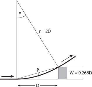
Figure 8.4. Geometry for turning to avoid a slower vehicle.

from which it follows that

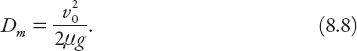
Examining this result, we note that it is independent of the mass (or weight) of the car. It is also proportional to the square of the initial speed; thus doubling the speed quadruples the minimum stopping distance. The value of the coefficient μ depends on the quality of the tires and the prevailing road conditions; probably the best realistic value is μ = 0.8, but for more worn tires, or wet roads, a somewhat lower value 0.7 or 0.6 is probably appropriate (or even lower for tires in poor condition). Here are some minimal (rounded) stopping distances for various speeds, taking μ = 0.65. Also included, for illustrative purposes, is D_r, the distance covered in a nominal (and somewhat slow) reaction time of one second. The fourth column is the approximate total distance (D_T) required to stop at these speeds, given the above assumption.

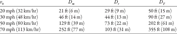
For simplicity we now consider a minimal stopping distance of 100 ft, corresponding to a speed of about 44 mph (71 km/hr). If the vehicle is able to pass the obstacle without braking at all, this maneuver will begin after the reaction time. This means that the vehicle can pass a large obstacle of width nearly 27 feet if traffic in the adjacent lane(s) permits. But then the direction of the car will be at an angle of 30° to the original direction, a dangerous predicament to be sure!

To improve the safety of this maneuver, consider the following modification: we require that once abreast of the obstacle, the car should be moving parallel to the road in the new lane. For this case, the geometry changes a little (see Figure 8.5). Now the car’s “trajectory” will be a sigmoidal-type shape composed of two smoothly joined circular arcs as shown. As before β = α/2, but now α = arcsin(1/4) ≈ 14.48°, so β ≈ 7.24°, meaning that the width of the obstacle should not exceed D tan β ≈ 0.127 D for the maneuver to be executable. For a value of D = 100 ft, this is just less than 13 ft, which allows for a few feet of clearance around a large truck.

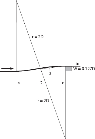
Figure 8.5. Modified geometry for turning to avoid a slower vehicle.

Next we consider two cars approaching an intersection perpendicularly at the same speed, as shown in Figure 8.6. Suppose that each driver instinctively tries to swerve to the side by at least 45°; we will take this as a lower bound, for then they end up moving parallel to each other (if road conditions permit, of course). The angles of the truncated triangle are each 45° and therefore by symmetry the line joining each vertex to the corner of the junction makes an angle exactly half this with the hypotenuse. Recall that the minimum distance required for a “straight stop” is D and that for a circular arc is 2D. Now the radius of the arc shown in Figure 8.6 is r = D cot(π/8) ≈ 2.41D. From equation (8.8) we can compare the corresponding speeds for the circular arc (1) and the 45° swerve (2):

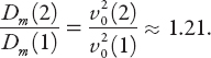
This implies that v₀(2)/v₀(1) ≈ 1.1, that is, the speed can be about 10% greater in the 45° swerve.

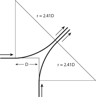
Figure 8.6. Two vehicles approaching on an initially perpendicular path.

A compromise of sorts between the straight stop of length D and the circular turn of radius 2D is the “spiral stop.” This is accomplished by turning and braking simultaneously, and the vehicle will trace out a spiral path. The straight stop is achieved by applying (in the simple case) a constant force at 180° to the direction of motion. The circular path arises when that force is applied at 90° to the direction of motion. When this force is applied at some other constant angle γ to the direction of motion, the result is an equiangular spiral trajectory. In polar coordinates the equation of the path takes the form r₁(θ) = r₀e^(2cotγ)θ, where r₀ is a constant (see Appendix 6 for details).

X = σ : ACCELERATION “NOISE” IN THE CITY

What factors are important in studying what might be called “traffic engineering”? Clearly, weather and road conditions and the driver’s response to a changing traffic environment are all significant and indeed, interrelated. A twisty two-lane road poses different problems from a six-lane Interstate highway or “main drag” in a city. The effects of increased traffic volume, road repairs, or adjacent building projects on congestion are generally difficult to answer quantitatively, but the concept of acceleration noise—the root-mean-square of the acceleration of a vehicle—is a useful one in determining some answers to questions of this type.

If v(t) and a(t) are respectively the speed and acceleration of a vehicle at time t, assumed continuous, then the average acceleration over a trip lasting time T is

It is interesting to note that if the initial and final speeds are the same, then ā = 0. This will certainly be the case if the vehicle starts from rest and stops at the end of the trip!

The acceleration noise σ is the RMS (root-mean-square) of a(t) − ā, that is,

Exercise: Show that

Clearly, when ā = 0, then

Exercise: Calculate this quantity for several simple analytic choices of a(t).

Why might this concept be a useful one for traffic engineering? If we think about a car that is driven fairly smoothly (i.e., with no violent acceleration or braking), we would expect the quantity σ to be small (in a sense to be discussed later). If the vehicle is driven with such accelerations and decelerations, σ will be large. Recall that the slope of a speed-time graph at a given point is the acceleration at that point. In effect, the acceleration noise is a measure of the smoothness of the speed-time graph—the smaller σ, the smoother the journey. A narrow, crowded road with sharp turns will give rise, other things being equal, to a higher value of σ. Those reckless drivers (never ourselves, of course) we see so frequently weaving in and out of traffic will engender high σ-values. Instead of wishing to shake a fist at them, or inwardly raging at them, perhaps we should just content ourselves with this fact. At this point, an amusing image comes to mind: after passengers alight from a car, they each in turn raise a card above their heads with an estimate of the σ-value for the just-completed trip!

In a very interesting article by Jones and Potts (1962), several possible answers to this question are provided, based on experimental data. After extensive investigations in Adelaide and its environs, they were able to draw several conclusions, some of them perhaps not surprising:

1. Given, say, a two-lane road and a four-lane road through hilly countryside, σ is much greater for the former than the latter.

2. For roads in hilly countryside, σ is smaller for an uphill journey than for a downhill one.

3. If two drivers drive at different speeds below the “design speed” of a highway, σ is about the same.

4. If one or both drivers exceeds the design speed of the highway, σ is higher for the faster driver.

5. An increase in the volume of traffic increases σ.

6. Similarly, an increase in traffic congestion resulting from parked cars, frequently stopping buses, cross traffic, pedestrians, etc., increases σ.

7. A suitably calibrated value of σ may provide a better measure of traffic congestion than travel or stopped times.

8. High values of σ indicate a potentially dangerous situation; they may be a measure of higher accident rates.

Naturally we must ask, what are typically high and low values for σ? The authors found that σ = 1.5 ft/s² is a high value, and σ = 0.7 ft/s² is a low one.

Another factor influenced by the size of σ is an economic one: fuel efficiency. This is not just important for trucking companies or individual truckers, of course: it is increasingly important for the average driver as well. Trucks are fitted with tachographs to record the driving behavior of the truckers, and presumably have the effect of providing an incentive to (in effect) lower the value of σ.

Generally, then, the smoothness of a journey can be measured by the acceleration noise—the standard deviation of the accelerations; furthermore, it is known that the acceleration distribution is essentially normal. It could well be a useful measure of the danger posed by erratic drivers, for whom σ is high. It also increases in tunnels, the reasons probably being narrow lanes, artificial lighting, and confined conditions. However, it is not always sensitive to changing traffic conditions, especially in city centers or major highways leading into them, where traffic congestion is common and the average speeds are low. It is also the case that a given value of σ may correspond to more than one traffic situation, for example, journeys at low speeds in dense traffic or faster journeys interspersed with traffic lights. One possibility to avoid this ambiguity is to use a modification of σ, namely , where is the average speed. may be interpreted as a measure of the mean change in speed per unit distance of the journey.

Question: jerk is defined as the time derivative of the acceleration, that is, j(t) = da/dt. Do you think there is any usefulness to defining a quantity similar acceleration noise (as in equation (8.10), namely jerk noise?

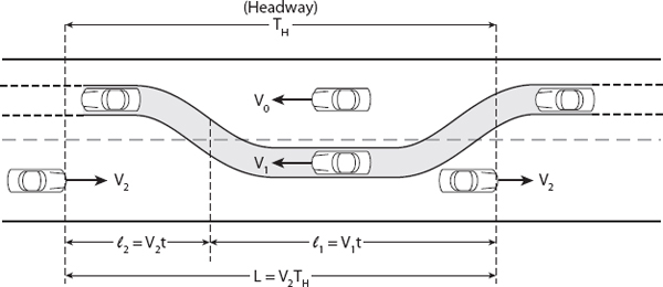
Figure 8.7. Headway geometry for a two-lane highway.

X = T_h: OVERTAKING IN THE CITY

We conclude this chapter with a simple mathematical model of overtaking and passing on a straight section of road. In Figure 8.7 a vehicle in the right lane moves into the left lane at speed V₁ > V₀ to overtake and pass a slower-moving vehicle. The equations, if not the diagram, are independent of which side of the Atlantic the vehicle resides! The headway T_H is the time gap between adjacent oncoming vehicles moving at speed V₂.

Clearly,

Suppose that a reasonable time in which to complete a passing maneuver by a car traveling at 55 mph is 8 seconds, the headway required for an oncoming vehicle traveling at 65 mph in the opposing lane is T_H ≈ 15 seconds. For interstates or other multilane highways, the needed gaps are smaller; we just change the sign of V₂ (obviously we require V₁ < V₂). In this case for the same speeds T_H ≈ 1.2 seconds!