Chapter 7
NOT DRIVING IN THE CITY!
As we have remarked already, cities come in many shapes and sizes. In many large cities such as London and New York, the public transportation system is so good that one can get easily from almost anywhere to anywhere else in the city without using a car. Indeed, under these circumstances a car can be something of an encumbrance, especially if one lives in a restricted parking zone. So for this chapter we’ll travel by bus, subway, train, or quite possibly, rickshaw. Whichever we use, the discussion will be kept quite general. But first we examine a situation that can be more frustrating than amusing if you are the one waiting for the bus.
X =T: BUNCHING IN THE CITY
In a delightful book entitled Why Do Buses Come in Threes? [8] the authors suggest that in fact, despite the popular saying, buses are more likely to come in twos. Here’s why: even if buses leave the terminal at regular intervals, passengers waiting at the bus stops tend to have arrived randomly in time. Therefore an arriving bus may have (i) very few passengers to pick up, and little time is lost, and it’s on its way to the next stop, or (ii) quite a lot of passengers to board. In the latter case, time may be lost, and the next bus to leave the terminal may have caught up somewhat on this one. Furthermore, by the time it reaches the next stop there may be fewer passengers in view of the group that boarded the previous bus, so it loses little time and moves on. For the next two buses, the cycle may well repeat; this increases the likelihood that buses will tend to bunch in twos, not threes.
The authors note further that if a group of three buses occurs at all (and surely it sometimes must), it is most likely to do so near the end of a long bus route, or if the buses start their journeys close together. So let’s suppose that they do . . . that they leave the terminal every T minutes, and that once they “get their buses in a bunch” buses A and B and B and C are separated by t minutes (where t < T of course). A fourth bus leaves T minutes after C, and so on. The four buses have a total of 3T minutes between them, initially at least. When the first three are bunched up, the fourth bus is 3T − 2t minutes behind C (other things such as speed and traffic conditions being equal). If you just missed the first or the second bus, you have a wait of t minutes for the third one; if you just missed that then you have a wait of 3T − 2t minutes. Thus your average wait time under these circumstances is just T, the original gap between successive buses!
How does this compare with not missing the bus? The probability that you have arrived in the long gap as opposed to one of the two short ones is (3T − 2t)/3T, your time of arrival could be just after the third bus left, just before the fourth one arrives, or any time in between, and the mean of those two extremes is (0 + 3T − 2t)/2. This will actually be longer than the previous average wait time if T > 2t, which of course is quite likely, even allowing for the small possibility that you arrived in a t-minute gap.
X = Va: AVERAGE SPEED IN THE CITY
We shall examine and “unpack” an idealized analysis of public transport systems (based on an article [14] published in the transportation literature). The article contained a comprehensive account of two models: a corridor system and a network system. In so doing, it is possible to derive some general results for transport systems. Although some of these conclusions were represented in graphical form only, the mathematics behind those graphs is well worth unfolding here. In both models there are three components to the travel time from origin A to destination B: (i) the walk times to and from the station at either end; (ii) the time waiting for the transportation to arrive; and (iii) the total time taken by the subway train, bus, or train to go from the station nearest A(SA) to that nearest B(SB). (This includes waiting time at intermediate stops along the way.)
In what follows, the city is assumed to have a “grid” system with roads running N-S and E-W (see Appendix 3 on “Taxicab geometry”). While this may be more appropriate to cities in the United States, it is also an acceptable approximation for many European cities [14], [15]. From Figure 7.1 we see that a walk from any location to any station will involve an N-S piece and an E-W piece. If each station is considered to be at the center of a square of side L, the average walk length is L/2. To see this, note that for any trip starting at the point (x, y) on the diagonal line (for which x + y = L/2) to the center is just L/2. By symmetry, there is the same area on each side of the line. If the population demand is uniformly distributed, L/2 is the average trip to or from the central station, and hence L is the average total distance walked—just the average stop separation.

Figure 7.1. One segment of a transportation corridor with a central station serving a square area of side L. The diagonal shown has equation x + y = L/2.
First we consider the average speed Va for the vehicular part of the trip. We suppose that this part consists of a uniform acceleration a from rest to a (specified) maximum speed Vm(A–B), and a period of travel at this speed (B–C–D) followed by a uniform deceleration −a to rest at the next station (D–E). The acceleration and deceleration take place over a distance x km, say, and the speed is constant for a distance L − 2x ≥ 0. Using the equations of motion for uniform acceleration it is found that Vm = (2ax)1/2 and the time Tx to travel the distance x (= distance AB) and reach this maximum speed is Tx = (2x/a)1/2. The time to travel the distance BC is therefore TBC = ([L/2] − x)/Vm. If we include a waiting time TW at the station A before leaving for the next one at E, the total time for the journey AE is 2 (Tx + TBC) + TW; typically, TW ≈ 20s and a = 0.1g according to published data [15]. Hence the average speed in terms of the maximum speed is
![]()
after a little reduction. We take TW = 20s and a = 10−3 km/s2 ≈ 1.3 × 10⁴ km/hr2 in what follows. Then equation (7.1) takes the form
![]()
where α = 7.7 × 10⁻⁵, β = 5.6 × 10⁻³.
It is interesting to note that on the basis of formula (7.2), Va possesses a shallow maximum occurring at ![]() for the constants chosen here. For a station separation L = 0.5 km this corresponds to Vm ≈ 80 km/hr. It can be seen from Figure 7.2 that for L = 1 km the maximum average speed attainable is only about 40 km/hr regardless of maximum speed. For a stop spacing of 0.25 km the maximum is less than 20 km/hr. In these cases the vehicle does not have enough time to reach its maximum speed and merely accelerates to the midpoint and then decelerates.
for the constants chosen here. For a station separation L = 0.5 km this corresponds to Vm ≈ 80 km/hr. It can be seen from Figure 7.2 that for L = 1 km the maximum average speed attainable is only about 40 km/hr regardless of maximum speed. For a stop spacing of 0.25 km the maximum is less than 20 km/hr. In these cases the vehicle does not have enough time to reach its maximum speed and merely accelerates to the midpoint and then decelerates.

Figure 7.2. Average speed vs. maximum speed for different values of station spacing L = 5 km, 2 km, 1 km, 0.5 km.
The next phase of the calculation is to include passenger “walk and wait” times, the latter referring to the wait for the arrival of the train or bus. Furthermore, a trip length is now assumed. We shall adopt 80 m/min or 4.8 km/hr for the average walking speed, the average passenger wait time as 5 minutes, and an estimate of 8 km for the average (UK) trip length [14]. The number of stops beyond the origin is 8/L (if this is an integer), as is the number of in-station wait times TW. For small values of L (less than 0.25 km, for example) the model is impractical, but we shall nevertheless treat L (and the number of stations) as a continuous variable. The average speed is now
![]()
Graphs of Va(L) for Vm = 30 km/hr and 80 km/hr are shown in Figures 7.3a and 7.3b, for comparison with the graph for the in-vehicle average speed without the passenger walk-and-wait times (the above expression without the last two terms in the denominator). The lower speed for Vm is representative of a bus, given the typical stops necessary at crosswalks (pedestrian crossings) and traffic lights. The higher speed is more typical of light rail, monorail, or possibly priority bus lanes, which would ensure higher average speed. From the figure it is seen that for the bus the optimum spacing L between stations (corresponding to the peak average speed) is about 0.5 km. For the higher speed, the optimum spacing is closer to 0.75 km.
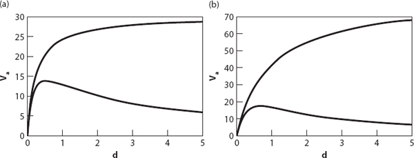
Figure 7.3. (a) Average speed vs. stop separation (in km) for maximum speeds of 30 km/hr for in-vehicle with stops (upper curve) and with walk and wait times included (lower curve). (b) Average speed vs. stop separation (in km) for maximum speeds of 80 km/hr for in-vehicle with stops (upper curve) and also with walk and wait times included (lower curve). The generic distance d in Figures 7.3–7.5 represents the spacing L between stops.
Note what little difference the increase in maximum speed makes to the maximum average speed. These average speeds are probably at best comparable to the average speed for cars in rush hour periods, since the latter will not have to keep stopping to let passengers on or off. This model suggests that overall trip times using public transport will generally be higher than for cars during the same peak times.
X = Lv: AVERAGE TRIP LENGTH IN THE CITY
Consider first an eastbound trip consisting of N stops, numbered from n = 0 to N − 1. The total number of such trips from 0 is N − 1, from 1 is N − 2, etc. so summing over all values of n we find that the total number of eastbound trips is the well-known result
![]()
The sum of all the trips from the mth stop eastward (0 ≤ m ≤ N − 1)can be found by replacing N above by N − m, that is,
![]()
If the stations are a distance L apart, then the sum of all trip distances from all stops is L times the sum of the above expression over all possible values of m, that is,
![]()
Exercise: establish the result (7.4).
For trips on a rectangular grid containing M stops on the N-S corridors, the total length of eastbound trips in any one row is M times the result (7.4) above, and the total length over all rows requires multiplication by M once more. Multiplying this by two for the westbound trips, the total length of eastbound and westbound trips is
![]()
Assuming a uniform demand at the MN starting points, each of which serves the MN − 1 others, there are MN(MN − 1) trips, so the average length of all eastbound and westbound trips is
![]()
By interchanging M and N we obtain the corresponding result for N-S trips, that is,
![]()
Any single trip will generally involve a combination of both types of trip, so the average length over all trips is
This gratifying result shows that the average trip length is one sixth of the perimeter of the area served, and if the area is square, this is two thirds of the length of a side.
With this general result established (though only for the in-vehicle part of the trip), we proceed with the “walk, wait, ride, and walk” overall trip time calculations for a square city of side c. With a grid containing n2 equally spaced stations, the distance between adjacent stops is c/n, and with each station centrally located in its “sub-square,” the average walk distance is, from our earlier discussion, c/2n, which of course must be doubled for the assumed symmetry of the trip. The time to walk both such trips is c/nW.
The “wait time” depends on the spacing of the vehicles on a line. For example, if they are two stations apart the wait time is 2c/nVa, and in general, sc/nVa for a vehicle spacing of s stations. The trip time is merely the average distance divided by Va, and from the previous discussion, this will be 2c/3Va. There is also a transfer time for travel involving different vehicles, which for our purposes is just the waiting time multiplied by a factor F of order one. (There are data [14] indicating that for networks sizes up to 10 × 10, 0.5 ≤ F ≤ 2. This will be generically incorporated in the term sc/nVa for the calculations below.)
Combining all three “times,” that is, walk + wait + in-vehicle, we express the overall trip time as
![]()
In keeping with the literature [14], we choose a city size of c = 10 km. In Europe, typical population densities are around [14] 4000/km2 (the average figure for U.S. cities is about half this). Thus “our” city has a population of about 400,000. The average length of all trips is, as noted above, 2/3 of the side length, approximately 6.7 km. Again, fictionally treating the station spacing as a continuous variable, we can the network travel time as a function of station spacing from the above formula.
The total travel time in minutes is shown in Figure 7.4 for Vm = 30 km/hr (upper curve) and 80 km/hr (middle curve). The lower (dotted) line is the walk time, and it can be seen that the walk time is the dominant contribution for large station spacing (corresponding to fewer tracks). Notice that the minimum travel time for the slower speed of 30 km/hr occurs at a stop spacing of about 0.25 km (appropriate for a city bus route) and at about 0.5 km for the 80 km/hr monorail route.
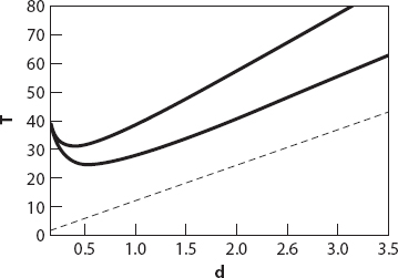
Figure 7.4. Total travel time (minutes) vs. stop spacing for a maximum speed of 30 km/hr (upper curve) and 80 km/hr (middle curve). The dotted line represents the walk time component for one end of the trip.

Figure 7.5. Average speeds in km/hr vs. stop spacing, based on Figure 7.4. The upper curve is for a maximum speed of 80 km/hr, the lower for a maximum speed of 30 km/hr.
Figure 7.5 shows the average speed for these curves (starting for d = L = 0.1 km). Note that the maximum average speed is only between about 13 and 16 km/hr for the range of maximum speeds considered here.
The much higher value for Vm of 80 km/hr adds relatively little to the average speed.
A final word: pedestrians. The most complete forms of the above models make allowances for the average time to walk to and from the station. As someone who has walked to work almost every weekday for twenty-eight years, I have learned to be very careful about crossing roads. I have to judge whether there is sufficient time to do so before the nearest vehicle reaches me. (One certainly hopes there is.) In fact, every individual has (in principle) a critical time gap, T say, above which crossing is acceptable and below which it is not. Mathematically, this can be represented by a step function
G(t) = 0, t ≤ T,
G(t) = 1, t > T.
I think a step function is an entirely appropriate thing for pedestrians to have.