
Chapter 13
CONGESTION IN THE CITY

If all the cars in the United States were placed end to end, it would probably be Labor Day Weekend.
—Doug Larson
X = v(N): SOME EMPIRICAL MEASURES OF URBAN CONGESTION
What percentage of our (waking) time do we spend driving? In the United States, a typical drive to and from work may be at least half an hour each way, frequently more in high density metropolitan areas. So for an 8-hr working day, the drive adds at least 12–13% to that time, during much of which drivers may become extremely frustrated. (Confession: I am not one of those people; I am fortunate enough to walk to work!)
On 25 January 2011 my local newspaper carried an article entitled “Slow Motion.” The article took data from the American Community Survey (conducted by the U.S. Census Bureau) and presented average commuter travel times for the region. According to the survey, the NYC metro area had the highest “average commute time,” more than 38 minutes; Washington, DC, was second with 37 minutes, and Chicago was third with more than 34 minutes. (The piece in the newspaper stated the commute times to the nearest hundredth of a minute—about half a second—which is clearly silly!) The average for my locality was about 26 minutes.
In much of what follows, the equations describing various features of traffic-related phenomena are based on detailed observational studies published in the literature. Consequently, the coefficients in many of these equations are not particularly “nice,” that is, not integers! For example, one measure of the capacity of a road network in a UK city center (London) was given by [25]
![]()
where v1 is the average speed of traffic in mph (numerically). The traffic flow is more easily appreciated by inverting this to give the approximate expression v1 = (523 − 7.7N)1/2. For comparison, another empirical measure is also illustrated:
![]()
As can be seen from Figure 13.1, the two formulae give similar results for speeds above about 12 mph, but in fact v1(N) (solid curve) is a better fit to the low-speed data. It should be emphasized that both N and v1,2 are numerical values associated with the units in which they are expressed, so equation (13.1) and others like it are dimensionless.
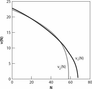
Figure 13.1. v1 and v2 in mph vs. N (cars/hr/highway width in ft)
Of course, not all vehicles will be cars. In some of the literature [20]–[27], bicycles were regarded as the equivalent of one third of a car, buses the equivalent of three cars, and so forth. Thus, in order to achieve a speed of v mph, equation (13.1) suggests that each car on the road, during a period of one hour, requires a width of (68 − 0.13v2)−1 ft. A bus would require three times this width and a bicycle one third (a motorcycle, presumably, one half).
GENERAL ALGEBRAIC EXPRESSIONS FOR TRAFFIC DYNAMICS
X = δT: Question: How are increases in traffic and losses in time (due to congestion) related?
As above, we’ll write N(v) as a quadratic function,
where N0 = a and ![]() = a/b. N0 is interpreted as the maximum flow of vehicles and v0 as the speed under “light” traffic conditions. Suppose that a journey is of distance l and we define T, the accumulated time loss due to congestion, as the difference (for N vehicles) between the times traveled at speeds v and v0, respectively, then
= a/b. N0 is interpreted as the maximum flow of vehicles and v0 as the speed under “light” traffic conditions. Suppose that a journey is of distance l and we define T, the accumulated time loss due to congestion, as the difference (for N vehicles) between the times traveled at speeds v and v0, respectively, then
![]()
We shall define the relationship between small changes in T and N (δT and δN respectively) by
![]()
where T′(N) is the derivative of T with respect to N. If T′ is not too large, a small change in N induces a correspondingly small change in T according to this formula. This is a slight variation on the definition of differentials in elementary calculus, but it will be quite sufficient an approximation for our purposes, and indeed a good one, so we will use “=” rather than “≈” in what follows. From equations (13.2) and (13.3) we obtain
or

As a function of the ratio v0/v, the right-hand side of (13.5) is a cubic polynomial, increasing monotonically from zero when the traffic is light (v0/v = 1). Graphically, it is perhaps easier to appreciate as a function of the ratio of speed to the “light” speed (not the speed of light!), that is, in terms of x = v/v0. Thus
![]()
The graph of this decreases monotonically to zero when x = 1, and as can be seen in Figure 13.2, the congestion term on the left of equation (13.6) decreases by a factor of about twelve as x increases from 0.2 to 0.5; that is, when the average speed is one fifth of the speed of light traffic, the time loss is about twelve times as great as when the average speed is one half that of light traffic. Furthermore, from equations (13.2), (13.3), and (13.5) we can deduce an expression for the following useful measure of congestion:
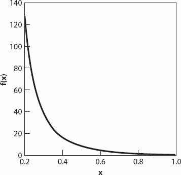
Figure 13.2. Graph of the function f(x) defined by equation (13.6).
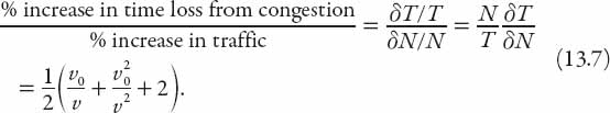
Clearly δT/T increases as a quadratic function of the percentage increase of traffic.
X = δt: Question: What difference will just one more vehicle make?
The change in time for a journey of length l and duration t = l/v when there is a small change δv in speed is given by δt = −lδv/v2. If this change arises because of a small change δN in the traffic flow, we may write
![]()
Therefore, if N is the flow before I try to sneak my car into the traffic, the total increase in journey time of the other vehicles is approximately Nδt/δN, that is, −Nlv′(N)/v2. I do feel a little guilty about this, but I have to get to the bank before it closes. Using equation (13.2) this can be rewritten as
![]()
We can extract more from this equation. The journey takes a time l/v, so that

As may be seen from equation (13.9), this represents a significant time loss if the speed of traffic is low. And here is another point to note: equation (13.8) represents the time loss imposed on other vehicles by my entry into the traffic stream. If we add to this the time loss sustained by my vehicle, then the resulting sum must be the same as that expressed by equation (13.5), that is,

Exercise: Verify this identity.
X = dx/dt: Question: How fast do traffic back-ups increase in length?
As we all know from experience, delays while driving can arise for several reasons: accidents or other obstructions, tunnels, bottlenecks at an intersection, raised bridges, or even a poorly adjusted traffic light at a busy junction. If the traffic flow is N vehicles at speed v, and joins a line of traffic (a traffic queue if you are reading this in the UK) with average flow N0 at speed v0, no line forms if N < N0. By contrast, if N > N0, a steadily increasing line forms (we are here excluding temporary back-ups that oscillate in length). In the latter case, the rate at which the line lengthens can be computed as follows. We denote the length of the back-up be x at time t, where x(0) = 0, that is, we suppose that the problem starts at time “zero.” Noting that the ratio N/v has units of (vehicles/hr) ÷ (mph), or vehicles/mile, it follows that at t = 0, a portion of road of length x contains Nx/v vehicles. At a later time t it contains N0x/v0, because of the back-up. Therefore the number of vehicles entering the stretch minus the number leaving it is (N − N0)t, but this is just the quantity ![]() . Hence the rate at which the back-up increases is
. Hence the rate at which the back-up increases is
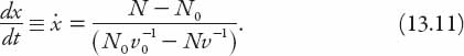
In the question below we apply this formula to an all-too-common situation in many parts of the world.
Question: Suppose the traffic is stationary. How fast is the line of traffic increasing?
This means that N0 = 0 and v0 = 0; clearly this means that equation (13.11) is indeterminate, so how are we to interpret the ratio N0/v0 in this case? Dimensionally, N/v is the ratio of vehicles per unit time to speed, that is, vehicles/length, or vehicular density on the road. In the case of stationary traffic, as here, this is just the concentration of vehicles in the queue. We shall take the effective length of an “average” vehicle to include the space between each one and the vehicle ahead. As before, we’ll call this density k, so equation (13.11) reduces to
![]()
This is the rate at which the traffic “jam” lengthens. Suppose, as an example, that we take the effective length for American vehicles (including the gap ahead) to be about 25 ft (it is probably less in Europe since the cars are typically smaller), and that the vehicles arrive at 30 mph, with a flow rate of, say, 500 vehicles per hour. The concentration per mile of the stationary line of cars, k, is then 5280 ÷ 25 ≈ 210 per mile. From (13.12) the line increases at a rate
![]()
Obviously, one can plug in one’s own estimates based on different traffic conditions.