Chapter 15

SEX AND THE CITY

 

 

We can think about the growth of cities in several ways, none of them prurient, despite the title of this chapter. Perhaps the most obvious one is how the population changes over time; another is how the civic area changes; yet another might be the number of businesses or companies in the city; and so on. These statistical properties are generally referred to as demographics, and they can include gender, race, age, population density, homeownership, and employment status, to name but a few. In this chapter we shall focus attention on some the simplest possible models of population growth in several different contexts, ending with some using “real” data from a bygone era. We’ll start with exponential growth.

X = P(t): MATHEMATICAL MODELS OF POPULATION GROWTH

In the November 4, 1960, issue of the journal Science, a paper [28] was published with the following provocative title: “Doomsday: Friday 13 November, A.D. 2026.” Beneath this was the sentence: At this date human population will approach infinity if it grows as it has grown in the last two millennia.

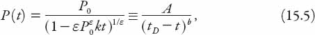
The authors presented a formula for the population P in terms of positive constants A, b, and t_D (to be defined below) as

In this equation, the subscript D stands for “Doomsday”! We proceed to derive more simply a form of this result to illustrate the principle behind it. But first, a caveat. In what follows, differential calculus is used. So what’s the problem with that? Well, in so doing, we are making the implicit assumption of differentiability, and hence continuity of the population of interest, whether it be humans, bedbugs, or tumor cells. But the populations are discrete! In these models, there are always an integral number of people, bedbugs, and so on. Calculus is strictly valid only when there is a continuum of values of the variables concerned and the dependent variables are differentiable functions. In that sense continuum models can never be totally realistic, even when there are billions of individuals (such as the number of cells in a tumor). Nevertheless, if there are sufficiently many individuals, we can justifiably approximate the properties of the population and its growth using calculus. Further informal discussion of one aspect of this “discrete/continuum” problem can be found in Appendix 8. Now we can begin!

Everyone has heard of “exponential growth” but not everyone knows what it means. It applies to (here, differentiable) functions P(t) for which the growth rate is proportional to P, or equivalently, the “per capita” growth rate is a constant, k. In mathematical terms

If we know that at some time t = 0 say, the population is P₀, then the solution of equation (15.1) is

If k < 0, then P decreases exponentially from its initial value of P₀. Such exponentially decreasing solutions are used in many algebra books to illustrate the phenomenon of radioactive decay. If k > 0 we see an immediate problem: the solution grows without bound as t → ∞. This is reasonably supposed to be unrealistic, because if P represents the population of a city, country, or the world, there is not an unlimited supply of resources to maintain that growth. In fact, the English clergyman Thomas Malthus (1766–1834) wrote an essay in 1798 stating that “The power of population is indefinitely greater than the power in the earth to produce subsistence for man.” This has been paraphrased to say that populations grow geometrically while resources grow arithmetically. Not surprisingly, exponential growth is sometimes referred to as “Malthusian growth.”

Let’s modify equation (15.1) just a little, and examine the innocuous looking first-order ordinary differential equation

(with P(0) = P₀ as before). For reasons discussed below we will restrict the parameter ε to the range −1 < ε < ∞. This simple looking nonlinear ordinary differential equation has some surprises in store for us, and in fact is sometimes referred to as the “Doomsday” equation. The first thing to do is integrate it to obtain

where C is a constant of integration. This can be found immediately by setting t = 0 in equation (15.4). After a little rearrangement, the solution to equation (15.3) is found to be

with the restriction on t being

Equation (15.5) is in precisely the form stated at the beginning of this subsection.

Exercise: Derive the solution (15.5).

Before we examine some of the implications of this solution, and restrictions on it (remember: every equation tells a story), let’s reexamine equation (15.3) and plot the quantity k⁻¹dP/dt = P^1+ε ≡ r_i, i = 0, 1, 2, as a function of P for the three cases ε > 0, ε = 0, and −1 < ε < 0, respectively. This last inequality ensures that the population growth rate for this case is not declining, since

In Figure 15.1 these values correspond to the top, middle, and bottom curves. The case ε = 0 (dashed line) clearly corresponds to the equation for exponential growth we have already seen (equation (15.2)). The upper curve corresponds to the arbitrary (and for illustrative purposes, rather large) value for ε of 0.5.

 

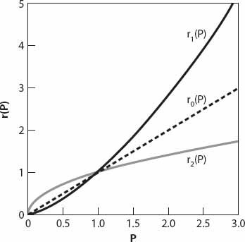
Figure 15.1. Curves proportional to the growth rates for super-exponential, exponential, and sub-exponential growth (from equation (15.3)).

The lower curve has ε = −0.5. Now let’s consider a much smaller but positive value of ε, 0.05 say. Then the growth is just slightly “super-exponential” with the right-hand side of equation (15.3) increasing in proportion to P^1.05. From equation (15.5) the solution is

This solution is undefined (“blows up”!) at time

in whatever units of time are being used (usually years, of course). This doomsday time is the finite time for the population to become unbounded. Thus if we take the current “global village” world population of 7 billion (as declared on October 31, 2011) to be P₀, and, for simplicity, an annual growth rate k = 0.01 yr⁻¹ (just 1% per year) then for the (admittedly arbitrary) value ε = 0.15, equation (15.7) gives

This is the doomsday time for our chosen value of ε! Note that if ε ≤ 0 the problem does not arise because there is no singularity in the solution. The population will still tend to infinity, but will not become infinite in a finite time, as is predicted for any ε > 0, no matter how small. The original “doomsday” paper [28] (and others listed in the references) should be consulted for the specific demographic data used.

Despite such a projection, I thought there was no suggestion that the world population is actually growing according to equation (15.3) until I read a paper [29] published in 2001. The first two sentences from the abstract of that paper may serve to whet the reader’s appetite for further discussion later in this book (Chapter 18): “Contrary to common belief, both the Earth’s human population and its economic output have grown faster than exponential, that is, in a super-Malthusian mode, for most of known history. These growth rates are compatible with a spontaneous singularity occurring at the same critical time 2052±10 signaling an abrupt transition to a new regime.” Doomsday again?

Exercise: Obviously the choice ε = 0 in equation (15.3) results in the standard exponential growth of P as noted above. Using a limiting procedure in equation (15.5), show that

Exercise: Another model, the “double exponential” model of bounded population growth, is defined by

where P_∞ is the asymptotic population (approached as t → ∞), 0 < b < 1, and 0 < a < 1.

(i) Show that

  (ii) A town population starts at P(0) = 80,000 and has an upper bound P_∞ = 200,000. It is known that after 10 years the population has risen to 150,000. Determine the constants a and b.

 (iii) Find the population after 15 years.

X = x(t): ANOTHER SIMPLE NONLINEAR MODEL—THE LOGISTIC EQUATION

Now we shall discuss a population model that predicts a definite limit on growth. Let’s examine the logistic differential equation

both k and N are positive constants. We have changed the dependent variable from P to x to reflect the fact that these models can apply to many different things. N is often called the carrying capacity in ecological contexts and the saturation level in chemistry. It can be used to describe, in a very simple manner, the spread of diseases or rumors in a closed community of population N, or a cultural fad, or indeed the spread of anything that can be spread by casual person-to-person contact, from the common cold to word-of mouth advertising about a new brand of coffee! (See Appendix 8.) The variable x(t) describes the number of individuals with the disease, or who have heard the rumor, read the ad, and so on, and for our purposes the most relevant range of values for x is 0 < x < N. The case x > N is also easily accommodated and will be discussed below. Equation (15.8) is separable, and using partial fractions we can integrate it to obtain

D being a constant of integration to be determined. Hence

where we have defined K = e^D. The general solution x(t) is therefore

Now rumors don’t start and diseases don’t spread without someone to initiate them, so we define the initial value of x to be x(0) = x₀ > 0. This enables us to find K in terms of the (in principle known) quantities x₀ and N. Thus

On rearranging the final result, the solution becomes

Check that the initial condition is satisfied, and note also that lim_t→∞ x(t) = N. This means that x = N is a horizontal asymptote; if nothing else changes, then the population x approaches the limiting value N from below (in this case) as time increases. Note that the solution (15.9) is still valid if x₀ > N; now the solution decreases monotonically from its initial value toward the asymptote from above. This case is meaningless in the present context, though it can apply to a simple model of overpopulation when the natural resources in a nature reserve, say, become compromised, perhaps by pollution or an environmental disaster. Then the normally sustainable population can no longer be supported, and the numbers decrease toward the new carrying capacity.

Further information about the evolution of x(t) may readily be found from examining both its population growth rate and its per capita growth rate using equation (15.8). The latter rate is just

and clearly in the interval 0 < x < N this is a linearly decreasing function. This means that the per capita growth rate slows uniformly from a maximum near kN (when x is small) toward zero as the carrying capacity (or saturation level) is approached. On the other hand, it can be seen from equation (15.8) that the population growth rate dx/dt as a function of x is a downward facing parabola with intercepts at x = 0, N and a maximum of kN²/4 at x = N/2.

X = ugh!: BED BUGS (OR RATS) IN THE CITY

We can now change the context somewhat from the spread of rumors and diseases to a city-related version of harvesting or fishing. Suppose that a city has a problem with vermin—whether of the four-legged, six-legged (bed bugs!), or winged variety (e.g., pigeons), and a program is introduced to reduce the population of these unwanted “critters.” How might we incorporate this “vermin reduction program” into the equations we have been discussing above? We can do this mathematically in two straightforward ways, depending on how the program is administered: by including a constant reduction rate or including a term proportional to the existing vermin population. Were we to replace “vermin” by “fish” then we would note that the former more appropriately describes a fishing effort in which the rate at which fish are caught on each fishing foray is the same. In the latter case the catch rate is proportional to the population, and the number of fish caught will thus diminish or increase as the population does. Taking the latter case first because it is mathematically simpler, and possibly more relevant to a town or city with a vermin problem, we can modify equation (15.8) as

Here the term cx represents the vermin reduction rate (in units of e.g. rats/week). The constant c can be thought of as the per capita reduction rate (rat?) resulting from the program. Noting that equation (15.10) may be rewritten as

where = N − c/k, we see that this has been encountered above; equation (15.11) is just (15.8) with a reduced carrying capacity (we assume that c ≤ Nk). The solution (15.9) still applies with this new horizontal asymptote replacing the earlier one. Nevertheless, this reduction is obviously helpful in the relentless fight against foul vermin! In terms of the original capacity N, the maximum growth rate is k(N − c/k)²/4 and occurs at x = (N − c/k)/2.

Returning to the constant reduction rate, we now have a governing equation

To study this, we write the quadratic polynomial on the right-hand side of (15.12) as P_c(x) in the form

Now P_c(x) possesses real zeros if and only if N²/4 > c/k, that is, if c < kN²/4. Then these zeros occur at

Clearly, P_c(x) > 0 when x₋ < x < x₊ as opposed to the case for c = 0, that is, where P₀(x) > 0 when 0 < x < N. Another way of thinking about this is by noticing that the right-hand side of equation (15.12) is just the original quadratic function kx(N − x) “lowered” by the amount c. This is illustrated in Figure 15.2 for x in units of N (or equivalently, N = 1) and k = 1, c = 0.15.

Recalling that P_c(x) = dx/dt, we can easily see from the figure that for c ≠ 0 (dotted curve), dx/dt < 0 for both x < x₋ and x > x₊. This means, according to this simple model, that the population of rats, bedbugs, or whatever it is declines to zero or to x₊. Obviously the former is the more desirable of the two situations. Furthermore, if c > kN²/4 then dx/dt for all x-values and the vermin population declines continuously to zero. This might reasonably be termed “overkill”!

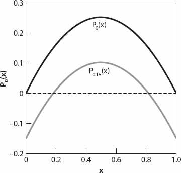
Figure 15.2. Right-hand side of equation (15.12) for c = 0 and 0.15 (solid and dotted curves respectively).

Exercise: Show that the solution of equation (15.12) is given by

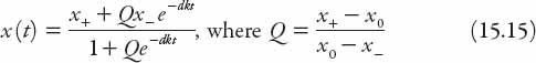
and d is the difference of the zeros of P_c(x), namely, x₊ − x₋. When c = 0, x₊ = N, and x₋ = 0 also verify that result this reduces as it should to the solution (15.9). The graphs of x(t) in units of N are shown in Figure 15.3 for both c = 0 (solid curve) and c = 0.15 (dashed curve), with k = 1 and x₀ = 0.25. Each exhibits the classic “logistic curve” sigmoid (or stretched S) shape.

X = ∑N: HOW MANY PEOPLE HAVE LIVED IN LONDON?

Well, I was one of them, but enough about me. Suppose that at time t₁ the population was N₁, and at a later time t₂ the population was N₂. Assuming that the growth was exponential, the annual growth rate r can then be determined from these data using the equation

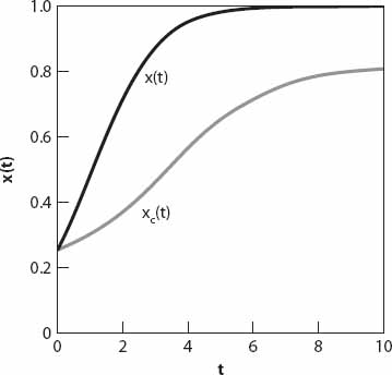
Figure 15.3. Solution curves from equation (15.15) for c = 0 and 0.15.

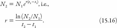
At any time t during the interval [t₁, t₂] the population was N₁e^r(t−t₁) and the total number of “person-years” from t₁ to t₂ is therefore

Hence the number of person-years lived is, from (15.16),

The left-hand side, expressed in person-years, can be converted to persons by dividing by a time factor. This should be an average life expectancy, but that is very difficult to determine, even if known in principle, owing to gender, regional, and temporal variations. For example, extracting possibly relevant (i.e., Northern European) data from a table in the Encyclopedia Britannica (1961), we have:

In view of these “data” we shall take an average of r⁻¹ = 40 years for the range 1801–2006 considered in Table 15.1, and estimate the quantity

TABLE 15.1

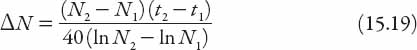
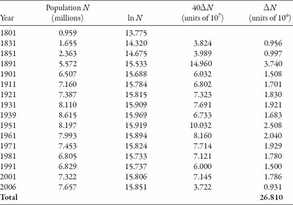
for a range of data points. Summing all these from the table we have the estimate of

Clearly this is a rough-and-ready approach, dependent on the width of the time intervals and the reliability of the data. The result is not particularly sensitive to the choice of life expectancy, but it is sensitive to the number of intervals chosen in the overall time frame. The more intervals we choose, assuming the data are available, the more different the cumulative population will generally be. To see this, just take a single interval from 1801 to 2006. We take t₁ = 1801 and t₂ = 2006, and N₁ = 9.59 × 10⁵, N₂ = 7.66 × 10⁶. Using equation (15.19), we find that N_tot (now equal to ΔN of course) ≈ 16.7 million. If we were to go back to the years t₁ = 1000 and t₂ = 2600 as before, then N₁ ≈ 10⁴ and N₂ is again as before. The corresponding value of N_tot is now 290 million for the same value of r. Obviously the value for London’s population in the year 1000 is somewhat suspect, but this is just to illustrate the point regarding the interval width. The average lifetime was probably lower in medieval times, so if we set r⁻¹ = 30 yr then N_tot increases to 386 million.

Nevertheless, this is an interesting application of some simple mathematics, and is probably far more reliable than estimates of all the people who have ever lived (Keyfitz 1976)!