Chapter 11

CAR FOLLOWING IN THE CITY—I

Don’t some cars inevitably follow others, and not just in the city? They certainly do, but the phrase as used here means that we model traffic by identifying each car as a separate object, not just part of the flow of a fluid called “traffic.” We’ll start by setting up a particular type of differential equation for this (now) discrete system.

X = x_n (t): A STEADY-STATE CAR-FOLLOWING MODEL

Suppose that the position of the nth car on the road is x_n(t). If we disallow passing in this model we can assume that the motion of any car depends only on that of the car ahead. A simple approach is to set the car’s acceleration proportional to the relative speed between it and the car in front; thus we have

This means that if the nth car is traveling faster than the one in front, it must decelerate to avoid a collision (generally a good idea). Conversely, if it is not traveling as fast as the one in front, the driver will (in this model) accelerate accordingly. Note that the model, simplistic as it is, does not give the driver the choice of maintaining a constant speed unless the right-hand side of equation (11.1) is zero. Additionally, the equation takes no account of the time lag due to the reaction time (T) of the driver in responding to the changing conditions ahead of her.

(At this point the reader may throw up his hands in disgust and say—“These mathematicians! Nothing is ever realistic—when do such conditions ever occur?” He has my sympathies, but this is the way modeling is usually done: take the simplest nontrivial situation and see what the implications are for the real-world problem, and modify, tweak, and improve as necessary . . . trial and error are important in constructing models.)

Incorporating the reaction time T results in the modification

According to one source, T is approximately 1.5 seconds for half of all drivers, and in the range 1–2.2 sec for all drivers, though over two seconds seems rather high to me. Equation (11.2) is actually a system of delay-differential equations (n = 1, 2, 3, . . .) and in general these are notoriously difficult to solve. It can be integrated directly however, to yield

where c_n is a constant of integration. This equation defines the speed of the nth car in terms of the separation from the car in front at an earlier time. Let’s examine the special case of a steady state (or time-independent) situation in which all the cars are spaced equidistantly, and hence moving at the same speed. Then, since

equation (11.3) may be reformulated as

We may now ask how the spacing x_n(t) − x_n−1 (t) = −d might depend on the traffic concentration k. In the situation described by equation (11.4), consider all vehicles to have length l, so that the number of cars per mile (or km) will be the constant value k = (l + d)⁻¹. From equation (11.4) with c_n = c

Imposing the reasonable requirement that at the maximum possible density k_max (bumper-to-bumper traffic), u = 0, we can solve for the constant c to obtain the simple result

There is a problem, however; this equation predicts that u → ∞ as k → 0(!). But it is easily resolved, because we know that for small enough densities, 0 < k < k_c say, u ≈ u_max. By requiring u(k) to be continuous it is necessary to choose

so that the traffic flow is

A typical q-k graph is shown in Figure 11.1. It is a piecewise linear approximation to the concave-down curve discussed in the previous model. One unfortunate feature is that the maximum flow occurs at k = k_c, which is unlikely to be the case. The corresponding u-k graph is shown as a dotted line.

The above model is rather limited in its scope, and can be improved somewhat by modifying the proportionality parameter b. This is likely to depend on the distance between the car and the one it is following; it seems reasonable to conclude that the closer it follows, the larger will be the accelerative or decelerative response. This quantity is in effect a sensitivity term. To this end, we choose

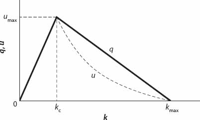
Figure 11.1. q(k) and u(k) profiles based on equations (11.6) and (11.5), respectively.

so that instead of the linear equation (11.2) we have the following nonlinear version:

As above, this can be integrated, yielding

Again, we choose a steady-state traffic flow for which this reduces to

Since

we simplify this to the case when the traffic density is much less than the bumper-to-bumper density k_max = l/l (for which u = 0), that is, k l/l. Then (11.9) reduces to

upon which, as before, we impose the low density condition u = u_max to avoid singular behavior as k → 0. The flow is therefore given by

For u to be continuous the choice of

must be made, but in this model the coefficient B has a more interesting interpretation. From equation (11.10) the maximum flow occurs when

and this occurs when k = k_max/e. At this value of k, the speed of traffic is, from (11.10) simply u(k_max/e) = B. For consistency with the continuity requirement, k_c must be such that

or more explicitly,

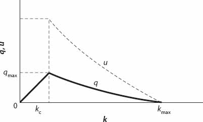
Figure 11.2. q(k) and u(k) profiles based on equations (11.11) and (11.10), respectively.

A generic sketch of both u(k) (dotted line) and q(k) is shown in Figure 11.2.