Appendix 10

RANDOM WALKS AND THE DIFFUSION EQUATION

Consider the motion of non-interacting “point particles” along the x-axis only, starting at time t = 0 and x = 0 and executing a random walk. The particles can be whatever we wish them to be: molecules, pollen, cars, inebriated people, white-tailed deer, rabbits, viruses, or anything else as long as there are sufficiently many for us to be able to assume a continuous distribution, and yet not so dense that they interact and interfere with one another (though this may seem rather like “having our cake and eating it”!). In its simplest description the particle motion is subject to the following constraints or “rules”:

1. Every τ seconds, each particle moves to the left or the right, moving at speed v, a distance δ = ±vτ. We consider all these parameters to be constants, but in reality they will depend on the size of the particle and the medium in which it moves.

2. The probability of a particle moving to the left is ½, and that of moving to the right is also ½. Thus they have no “memory” of previous steps (just like the toss of a fair coin); successive steps are statistically independent, so the walk is not biased.

3. As mentioned above, each particle moves independently of the others (valid if the density of particles in the medium is sufficiently dilute).

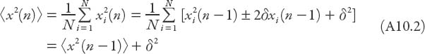
Some consequences of these assumptions are that (i) the particles go nowhere on the average and (ii) that their root-mean-square displacement is proportional, not to the time elapsed, but to the square root of the time elapsed. Let’s see why this is so. With N particles, suppose that the position of the ith particle after the nth step is denoted by x_i(n). From rule 1 it follows that x_i(n) − x_i(n − 1) = ±δ. From rule 2, the + sign will apply to about half the particles and the − sign will apply to the other half if N is sufficiently large; in practice this will be the case for molecules. Then the mean displacement of the particles after the nth step is

That is, the mean position does not change from step to step, and since they all started at the origin, the mean position is still the origin! This means that the spread of the particles is symmetric about the origin.

Let’s now consider the mean-square displacement . It is clear that

so that

Since x_i(0) = 0 for all particles i,

Thus the mean-square displacement increases as the step number n, and the root-mean-square displacement increases as the square root of the step number n. But the particles execute n steps in a time t = nτ so n is proportional to t. Thus the spreading is proportional to . And as we have shown in Chapter 19 for the case of a time-independent smokestack plume or a line of traffic, the spreading is proportional, in the same fashion, to the square root of distance from the source.

Incidentally, there is a very nice application of these ideas, extended to three dimensions, in the book by Ehrlich (1993). In an essay entitled “How slow can light go?” he points out that, barring exotic places like neutron stars and black holes, it’s probably in the center of stars that light travels most slowly. This is because the denser the medium is, the slower is the speed of light.

In fact, it takes light generated in the central core of our star, the sun, about 100,000 years to reach the surface! (Do not confuse this with the 8.3 minutes it takes for light to reach Earth from the sun’s surface.) The reason for this long time is that the sun is extremely opaque, especially in its deep interior. This means that light travels only a short distance (the path length) before being absorbed and re-emitted (usually in a different direction). The path of a typical photon of light traces out a random walk in three dimensions, much like the two-dimensional path of a highly inebriated person walking away from a lamppost. After a random walk consisting of N steps of length (say) 1 ft each, it would be very unlikely for the person to end up N feet away from the lamppost. In fact the average distance staggered away from the lamppost turns out to be feet.

In the sun, the corresponding path length is about 1 mm, not 1 foot. This is the average distance light travels before being absorbed, based on estimates of the density and temperature inside the sun. The radius of the sun is about 700,000 km, or 7 × 10⁵ km, or approximately 10¹² mm, rounding up for simplicity to the nearest power of ten. Now watch carefully: there’s nothing up my sleeve. We require this distance, the radius of the sun, to be the value of , the distance from the center traveled by our randomly “walking” photon. This means that N ≈ (10¹²)² = 10²⁴, and 10²⁴ mm steps is 10¹⁸ km. Now 1 light year is about 10¹³ km (check it for yourself!), so N ≈ 10⁵ light years, which by definition takes 10⁵ or 100,000 years! Good gracious me!

THE DIFFUSION EQUATION

Now we formulate the one-dimensional diffusion equation in a very similar fashion. Basically, we wish to be able to describe the “density” of a distribution of “particles” along a straight line (the x-direction) as a function of time (t). N(x, t) will denote the density of particles (number per unit volume) at location x and time t. How many particles at time t will move across unit area perpendicular to the x-direction from x to x + δx? By the time t + τ (i.e., during the next time step), half of the particles will have moved to the location x + δ and half of those located at x + δ will have moved to x (see Figure A10.1). This means that the net number moving from x to x + δx is [N(x,t) − N(x + δ, t)]/2. The total number of these particles per unit time and per unit area is called the net flux. We’ll call this F_x and rearrange it as

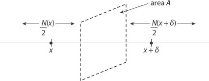
Figure A10.1. Schematic for the flux argument leading to equation (A10.4).

The quantity δ²/2τ has dimensions of (distance)²/(time), and this will be called the diffusion coefficient D. The first quotient in square brackets is the number of particles per unit volume at x + δ and time t. This is just the concentration, denoted by C(x + δ,t). Similarly, the second term is C(x,t). This means that we can rewrite the net flux as

At this point we are in a position to carry out a familiar procedure: taking the limit of this quotient as δ → 0. If this limit exists, we can write

Physically this means that the net flux is proportional to the concentration gradient, and it moves in the opposite direction. We can think of it this by imagining instead that C is temperature; the flow of heat will be from the higher temperature region toward the lower one—in a direction opposite to the gradient of the temperature. If on the other hand C is the concentration of sugar in my tea, the flow of sugar molecules is toward regions of lower concentration.

Let’s take this one stage farther and consider a little slab of thickness δ and area A perpendicular to the x-axis (see Figure A10.2). In a time τ, the number of particles entering from the left is F_x(x)Aτ, while F_x(x + δ)Aτ leave from the right (assuming no particles are created or destroyed). This means that the number of particles per unit volume in the slab must increase at a rate given by the expression

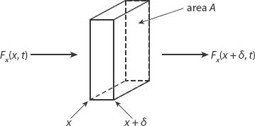
Figure A10.2. Schematic for the flux argument leading to equation (A10.6).

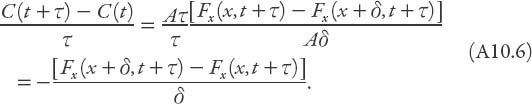
In the limit τ → 0, δ → 0 we obtain

There is another mechanism that must be included in any realistic discussion of pollution: wind. As with the discussion in Chapter 19 we shall consider the effects of a wind with constant speed U in the x-direction only (even when a higher-dimensional diffusion equation is used). The rate at which particles enter the slab per unit volume is approximately UC(x, t)A, so the wind’s contribution to the right-hand side of the diffusion equation is approximately

And so in the usual limit, equation (A10.7) is generalized slightly to become