Chapter 3

LIVING IN THE CITY

 

 

X = N: A “ONE-FITS-MANY” CITY “BALLPARK” ESTIMATE

Suppose the city population is N_p million, and we wish to estimate N, the number of facilities, (dental offices, gas stations, restaurants, movie theaters, places of worship, etc.) in a city of that size. Furthermore, suppose that the average “rate per person” (visits per year, or per week, depending on context) is R, and that the facility is open on average H hours/day and caters for an average of C customers per hour. We shall also suppose there are D days per year. This may seem a little surprising at first sight: surely everyone knows that D = 365 when the year is not a leap year! But since we are only “guesstimating” here, it is convenient to take D to be 300. Note that 400 would work just as well—remember that we are not concerned here about being a “mere” factor of two or three out in our estimate.

Then the following ultimately dimensionless expression forms the basis for our specific calculations:

For simplicity, let’s consider a city population of one million. How many dental offices might there be? Most people who visit the dentist regularly do so twice a year, some visit irregularly or not at all, so we shall take R = 1, C = 5, H = 8 and D = 300 (most such offices are not open at weekends) to obtain

That is, to the nearest order of magnitude, about a hundred offices. A similar estimate would apply to doctors’ offices.

Let’s now do this for restaurants and fast-food establishments. Many people eat out every working day, some only once per week, and of course, some not at all. We’ll use R = 2 per week (100 per year), but feel free to replace my numbers with yours at any time. The size of the establishment will vary, naturally, and a nice leisurely dinner will take longer than a lunchtime hamburger at a local “McWhatsit’s” fast-food chain, so I’ll pick C = 50, allowing for the fast turn-around time at the latter. Hours of operation vary from pretty much all day and night to perhaps just a few hours in the evening; I’ll set an average of H = 10. Combining everything as before, with D equal to 400 now (such establishments are definitely open on weekends!), we find for the same size city

Therefore the most we can say is that there are probably several hundred places to eat out in this city! I’m getting hungry . . .

We can do this for the number of gas stations, movie theaters, and any other facility you wish to estimate.

Exercise: Make up your own examples. Do your answers make sense?

Our final example will be to estimate the number of houses of worship in the city. Although many, if not most, have midweek meetings in addition to the main one at the end of the week or at some time during the weekend, I shall use the figure for R of 50 per year (or once per week) as above in the “eating out” problem. Spiritual food for those that seek it! But now I shall include the proportion of people who attend houses of worship in the calculation because clearly not everyone does. In the U.S. this is probably a higher proportion than in Europe, for example, so I shall suggest that one in five attend once per week in the U.S. The estimates for C and H are irrelevant (and meaningless) in this context, since everyone who attends regularly knows when the services start! Furthermore, this is more of a “discrete” problem since the vast majority of those who attend a house of worship do so once a week, so we shall simplify the formula by estimating an average attendance for the service. From my own experience, some churches have a very small attendance and some are “mega-churches,” and I will assume that the range is similar for other faith traditions also. Using the Goldilocks principle—too small, too large, or just right?—I shall take the geometric mean of small attendance (10) and large attendance (1000), that is, 100. Hence the approximate number of houses of worship in a city of one million people is

X = d: THE MUSEUM

Question: What is the optimal distance from which to view a painting/sculpture/display?

At the outset, it should be pointed out that we are referring to an object for which the lowest point is above the eye level of the observer: a painting high on a wall, a sculpture or statue on a plinth, and so forth. Commonsense indicates that unless this is the case, the angle subtended by the statue (say) at the observer’s eye will increase as the statue is approached. Of course, there is still an optimal viewing distance—wherever the observer feels most comfortable standing or sitting—but this is subjective. What this question means is where is the maximum angle subtended when the base or bottom of the painting is above the ground? That a maximum must occur is again obvious—far away that angle is very small, and close up it is also small, so a maximum must occur somewhere between those positions.

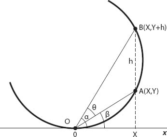
Figure 3.1. Display geometry for the maximum viewing angle. The object (e.g., a painting) lies along the vertical segment AB.

This is posed as a standard optimization problem in many calculus books. Consider the object of interest to be of vertical extent h (from A to B) with its base a distance Y above the observer’s eye line (the x-axis, with the observer at the origin O). From Figure 3.1 it is clear that the angle AÔB = θ = α − β is to be maximized. If A has coordinates (x, Y) in general, it follows that

Therefore an extremum occurs when

Y[x² + (Y + h)²] = (Y + h)(x² +Y²), i.e., when x = (Y² + Yh)^1/2 ≡ X.

We know this corresponds to a maximum angle, so we leave it to the reader to verify that θ″(X) < 0. For the Statue of Liberty, the plinth height Y is 47 meters, and the Lady herself is almost as tall: h = 46 meters. Therefore if the ground is flat we need to stand at a distance of X = (46 × 47 + 47²)^1/2 = 66 meters.

It is interesting to verify that the points O, A, and B lie on a circle: if this is the case, the center of the circle has coordinates (0, Y + h/2) by symmetry. Then if the radius of the circle is r it follows that

It is readily verified that the points A(X, Y), B(X, Y + h), and O(0, 0) all satisfy this equation, so the eye level of the observer is tangent to the circle. And another interesting fact is that this maximum angle is attained from any other point on the circle (by a theorem in geometry). Of course, this is only useful to the observer if she can levitate!

This result for the “vertical” circle (Figure 3.1) has implications for a “horizontal” circle in connection with the game of rugby—the best position to place the ball for conversion after a try is on the tangent point of the circle (see the book by Eastaway and Wyndham [8] for more details; they also mention the optimal viewing of two other statues—Christ the Redeemer in Rio de Janeiro and Nelson’s Column in London).

X = T: THE CONCERT HALL

We have tickets to the symphony. It is well known that the “acoustics” in some concert halls are better than in others—a matter of design. A fundamental question in this regard is—how long does it take for a musical (or other) sound to die out? But this is a rather imprecise question. As a rough rule of thumb, for the “average” (and hence nonexistent) person, weak sound just audible in a quiet room is about a millionth as intense as normal speech or music, so we’ll define the reverberation time T in seconds as the time required for a sound to reach 10⁻⁶ of its original intensity (Vergara 1959). Clearly, the value of T depends on many things, particularly the dimensions of the room and how well sound is absorbed by the wall, floor, ceiling, and the number of people present. Suppose that as the sound is scattered (here meaning reflected and absorbed) and the average distance between reflecting surfaces is L feet. On encountering such a surface suppose that (on average) a proportion a of the intensity is lost. We will call a the absorptivity coefficient. If the original sound intensity is I₀, then the intensity after n reflections is

We’ll assume this to be an exact expression from now on. Then we naturally ask: when does I_n = 10⁻⁶ I₀? In other words, if (1 − a)ⁿ = 10⁻⁶, what is n (to the nearest integer)? It is convenient to work with common logarithms here, so

(to the nearest integer). If c (ft/s) is the speed of sound in air at room temperature and pressure, then on average over a distance L, sound will be reflected approximately c/L times per second. This enables us to write the reverberation time T as

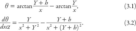
T is a linear function of L as we would expect, but before putting in some “typical” numbers, let’s see how the quantity N = n/6 = Tc/6L = −[log₁₀(1 − a)]⁻¹ behaves as a function of the absorptivity a.

It can be seen from Figure 3.2 and equation (3.6) that both n and T fall off rapidly for absorptivities up to about 20%. In fact, if we use c ≈ 1120 fps and L ≈ 20 ft, then n ≈ 270 and therefore the number of reflections per second is c/L ≈ 56 s⁻¹. This means that T ≈ 5 s, which is an awfully long time—almost long enough for the audience to leave the symphony hall in disgust! We need to do better than this. This is why soundproof rooms have walls that look like they are made of egg cartons: the value of a needs to be much higher than 0.05.

Figure 3.2. The reflection function n(a).

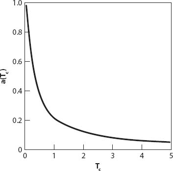
Figure 3.3. Absorptivity as a function of threshold reverberation time T_c.

However, we can invert the problem: suppose that the musicologists and sound engineers have determined that T should be no larger than T_c seconds. With the same values of c, and L, we now require that n = 56T_c, so that

For T_c = 1 s, a ≈ 0.22; for T_c = 0.5 s, a ≈ 0.39, and T_c = 0.1 s, a ≈ 0.92. That’s more like it! A graph illustrating the dependence of a on T_c is shown in Figure 3.3. Again, note the rapid fall-off when T_c < 1 s.

In reality, the physics of concert halls must be very much more complicated than this, but you didn’t really expect that level of sophistication in this book, did you?

X = R: SKYSCRAPERS

Figures 3.4 and 3.5 show, respectively, rebuilding at Ground Zero in New York City, and an office tower at Delft University of Technology in The Netherlands. In both cases we see tall buildings, very much taller than most kinds of trees. But trees sway in the wind, right? So why shouldn’t the same be true for tall buildings? In fact, it is true. The amplitude of “sway” near the top of the John Hancock building in Chicago can be about two feet. At the time of writing, the world’s tallest building has opened in Dubai. The Burj Khalifa stands 828 meters (2,716 ft), with more than 160 stories. It may not be long before even this building is eclipsed by yet taller ones. How much might such a building sway in the wind? Structural engineers have a rough and ready rule: divide the height by 500; this means the “sway amplitude” for the Burj Khalifa is about 5.5 feet! The reason for such swaying is intimately associated with the wind, of course; wind flows around buildings and bridges in a similar fashion to the way water flows around obstacles in a stream. Careful observation of this dynamic process reveals that small vortices or eddies swirl near the obstacle, be it a rock, twig, or half-submerged calculus book. The atmosphere is a fluid, like the stream (though unlike water, it is compressible) and buildings are the obstacles. If wind vortices break off the building in an organized, rhythmic fashion, the building will sway back and forth. Or, to put it another way, a skyscraper (or a smokestack) can behave like a giant tuning fork!

Figure 3.4. Rebuilding at the site of Ground Zero, New York City. Photo by Skip Moen.

Figure 3.5. Tower at the Delft University of Technology, Delft, The Netherlands. Photo by the author.

The oscillations arise from the alternate shedding of vortices from opposite sides of the tall structure. Their frequency depends on the wind speed and the size of the building. Not surprisingly, such “flow-induced” oscillations can be very dangerous, and engineers seek to design structures to minimize them [9]. Figure 3.6 illustrates in schematic form how such vortices can develop around a cylindrical body and alternatively “peel off” downstream.

There are two dimensionless numbers that are very important in a study of flow patterns around obstacles. One is called the Reynolds number, denoted by R, and is defined by

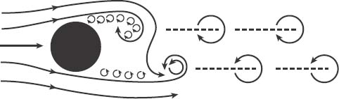
Figure 3.6. Schematic view of vortex formation around a cylindrical obstacle.

where L and U are characteristic size and (here) wind speed, respectively, and ν is a constant called the kinematic viscosity. For small values of R(R < 1) there is no separation: the cylinder just causes a symmetrical “bump” in flow. For R > 1 things get more complicated; in the range 1 < R < 30 small vortices develop behind the obstacle, but symmetrically about the axis of symmetry, so there is nothing yet to drive oscillations. For R > 40 this symmetric flow becomes unstable, and vortices are shed alternately from side to side (as viewed from above). This pattern can exist for Reynolds number up to several thousand (even up to 10⁵ if the obstacle is very “smooth”).

The other important number is the Strouhal number, S. It is named after Vincenc Strouhal, a Czech physicist who in 1878 investigated aeolian tones—the “singing” of wires set into oscillation by the wind. Again, in terms of the wind speed U and the diameter d of the wire, S is defined by

f_s being the frequency of the vortex shedding. Naturally it is to be expected that the Strouhal number is related to the Reynolds number, but for a wide range of the latter, S is almost constant, varying at most between 0.15 and 0.2. When f_s is close to the natural frequency of vibration of the obstacle, the latter can “capture” the former, and the resulting resonance can be very dangerous, for obvious reasons. This phenomenon is called “lock-in.”

And speaking of swaying buildings, a few minutes before I wrote this, my office building started to sway. I’m on the second floor, and didn’t feel anything, but I heard the bookcases behind me move back and forth. They have a lot of books in them, and are very heavy. Subsequently I heard tales from across campus of swinging lights and moving floors—yes, Virginia, we just had an earthquake! Initial reports indicated it was 5.8 on the Richter scale, with an epicenter midway between Charlottesville and and Richmond, Virginia (and about 80 miles from Washington, D.C.). Tremors were felt as far as New York, Massachusetts, Ohio, Tennessee. and the Carolinas, and the U.S. Capitol and the Pentagon were evacuated. And as I write, Hurricane Irene, currently a Category 3 storm, is making her way steadily toward the Eastern seaboard! Thankfully, by the time it made landfall the storm had weakened to Category 1, but it still caused one death and extensive property damage in the Outer Banks, North Carolina, New Jersey, New York, and Vermont.

X = d(x, y): THE MALL

Note that in the UK, mall = shopping center = shopping centre!

More and more frequently, malls are being located out of towns and cities, perhaps as a single “megastore” or as a mall-like complex; however, many are still built in cities with pedestrian walkways. What follows is a very simplistic model for the competitiveness of two such malls, carried out by considering how one “stacks up” against the other, as measured by the number of trips (N) made per unit interval to a given location.

An important (but rather subjective) question for urban planners is “How attractive is the mall likely to be?” Factors such as the variety of stores within it, ease of access, and parking facilities all contribute to the answer. Essentially, the attractiveness of the mall determines whether one will prefer to travel farther to get there, as opposed to shopping at a nearer but less attractive one. Another question, fundamental for developing a mathematical model for the competition between malls (or specialty stores and shops, for that matter) is “How does N depend on the distance d from the mall?” [10]. Many factors, including those mentioned above, must be contributory, and it is therefore unlikely that N will be a simple function of d. Nevertheless, that is beyond the scope of this book, and we shall content ourselves with a simpler approach to illustrate some basic principles involved.

Obviously we expect N to decrease with distance d, but how rapidly? Another question concerns what we mean by distance here, that is, should we use the standard Euclidean “metric” in the plane, or a modified version, weighted in some manner to account for geographical or social factors? In all likelihood the latter, but again for simplicity we will stick with circular symmetry, consistent with models that appear later in the book. (However, see Appendix 3 for a brief introduction to the so-called taxicab or Manhattan metric.) To that end, we define a constant “attraction factor” a_i > 0 for each mall (here i = 1, 2) and write

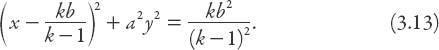
where the distance d(x, y) from a particular mall is calculated using the standard Pythagorean distance formula. The two malls A and B will be located at the coordinate origin and at (b, 0), respectively. We wish to determine the locus of points in the (x, y)-plane such that N₁ = N₂. This will be the (closed) boundary curve inside and outside of which one mall is preferred over the other. Therefore we can write

Rearranging this equation by raising both sides to the power 2/p we obtain

where the positive parameter k = (a₁/a₂)^2/p. In so doing we have effectively transferred the dependence on the distance (via the parameter p) to a measure of the “relative attractiveness” of the malls. For given values of a_i, note that k increases as p decreases toward zero if a₁/a₂ > 1, and k decreases as p decreases toward zero if a₁/a₂ > 1, and k decreases as p decreases toward zero if a₁/a₂ < 1. Upon completing the square it follows that for k ≠ 1

that is, the “boundary of attraction” is a circle of radius centered at the point . If 0 < k < 1, that is, mall A is considered less attractive than mall B, the center of the boundary is on the negative x-axis. Furthermore, in this case > k so that the circle extends into the half-plane and the point closest to mall B is at a distance from it. If k > 1, mall A is the more attractive of the two, and the closest point on the boundary to the point A is also a distance from it. Figure 3.7 illustrates this case for arbitrary k > 1; the dotted contours represent circular arcs on which (i) N₁ is constant (outside the solid circular boundary) and (ii) N₂ is constant (inside the boundary), respectively.

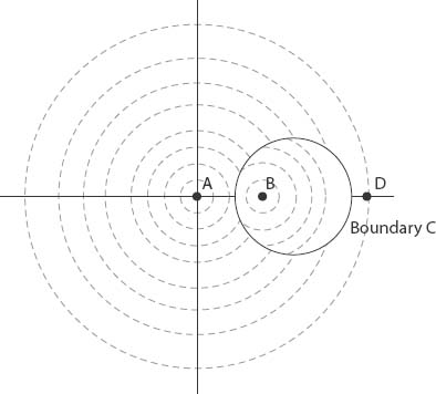
Figure 3.7. Equidistance contours and “attraction” boundary for a circular city.

One obvious and simple change to the model would be to consider elliptical contours of constant N_i; thus for the equation of the boundary curve we might use

instead of equation (3.9). In this case, if a > 1 the loci of constant N_i will be ellipses with semi-major axes along the x-axis, and the resulting boundary curve is also an ellipse, not surprisingly, with the equation

A representative diagram is shown in Figure 3.8.

X = P: THE POST OFFICE

I know that it’s usually a bad idea to go to the post office to mail letters when it first opens, especially on a Monday morning. And around the middle of December it’s a nightmare! But sometimes there is little or no line at all, even when the office is normally busy. That has happened on my last two visits. And conversely, sometimes there is a long line when I least expect it. While the average number of customers may be one every couple of minutes, it is most unlikely that each one will arrive every two minutes: there will be a certain “clumpiness” in the arrivals. The Poisson distribution describes this clumpiness well. Details and applications of this distribution are discussed in Chapter 9 and in Appendix 4, but we will summarize the results here. If the arrivals at the post office, checkout line, traffic line, busstops, and so on are random and average to λ per minute (or other unit of time), then the probability P(n) of n customers arriving in any given minute is

Figure 3.8. Equidistance contours and “attraction” boundary for an elliptical city.

Suppose that on a reasonably busy day at the post office, λ = 2. What is the chance that there will be six customers ahead of me when I arrive? (Of course, there is also the question of how quickly on average the counter clerks serve the customers, but that is another issue.)

Then

or just over 1 percent. That’s not bad! And that’s just for starters; we will meet the Poisson distribution again in Chapter 9.

X = Pr: CHANCE ENCOUNTER?

Another probability problem. Suppose that Jack and Jill, freshly arrived in the Big City, each have their own agendas about things to do. They decide—sort of—to do their “own thing” for most of the day and then meet sometime between 4:00 p.m. and 6:00 p.m. to have a bite to eat and discuss the day’s activities. Both of them are somewhat disorganized, and they fail to be more specific than that (after all, there are so many books to look at in Barnes and Noble, or Foyle’s Bookshop in London, who knows when Jack will be ready to leave?) Furthermore, neither cell (mobile) phone is charged, so they cannot ask “where the heck are you?”

Suppose that each of them shows up at a random time in the two-hour period. Jack is only willing to wait for 15 minutes, but Jill, being the more patient of the two (and frankly, a nicer person) is prepared to wait for half an hour. What is the probability they will actually meet? The related question of what will happen if they don’t is beyond the scope of this book, but the first place to start looking might be the local hospital.

This is an example of geometric probability. In the 2-hr square shown in Figure 3.9, the diagonal corresponds to Jack and Jill arriving at the same time at any point in the 2-hr interval. The shaded area around the diagonal represents the “tolerance” around that time, so the probability that they meet is the ratio of the shaded area to the area of the square, namely,

or about one third. Not bad. Let’s hope it works out for them.

X = Q(L, M): BUILDING IN THE CITY

To build housing requires land (L) and materials (M), and if the latter consists of everything that is not land (bricks, wood, wiring, etc.), then we can define a function Q(L, M),

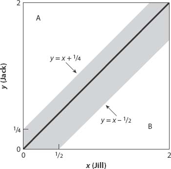
Figure 3.9. The shaded area relative to that of the square is the probability that Jack and Jill meet.

where a > 0 and 0 ≤ λ ≤ 1. This form of function is known as a Cobb-Douglas production function, widely used in economics, and named for the mathematician and U.S. senator who developed the concept in the late 1920s.

If the price of a unit of housing is p, the cost of a unit of land per unit area is l, and the cost of unit materials is m (however all these units may be defined), then the builders’ total profit P is given by

If a speculative builder wishes to “manipulate” L and M to maximize profit, then at a stationary point

Exercise: (i) Show, using equation (3.16), that this set of equations takes the algebraic form

(ii) Show also from equation (3.16) that according to this model, such a speculator “gets his just deserts” (i.e., P = 0)!

We shall use equations (3.15) and (3.17) to eliminate Q, L, and M to obtain

where C(α, λ) is a constant. With two additional assumptions this will enable us to derive a valuable result to be used in Chapter 17 (The axiomatic city). If the cost of materials is independent of location, and land costs increase with population density ρ according to a power law, that is, l ∝ ρ^κ(κ > 0), then

p = Aρ^γ,

where γ = κλ and A is another constant.

Exercise: Derive equation (3.18)

We conclude this section with a numerical application of equation (3.15) in a related context. It is recommended that the reader consult Appendix 5 to brush up on the method of Lagrange multipliers if necessary.

Suppose that

L now being the number of labor “units” and M the number of capital “units” to produce Q units of a product (such as sections of custom-made fencing for a new housing development). If labor costs per unit are l = $50, capital costs per unit are m = $100, and a total of $500,000 has been budgeted, how should this be allocated between labor and capital in order to maximize production, and what is the maximum number of fence sections that can be produced? (I hope the reader appreciates the “nice” numbers chosen here.)

To solve this problem, note that the total cost is given by

The simplified equation will be the constraint used below. The problem to be solved is therefore to maximize Q in equation (3.19) subject to the constraint (3.20). Using the method of Lagrange multipliers we form the function

The critical points are found by setting the respective partial derivatives to zero, thus:

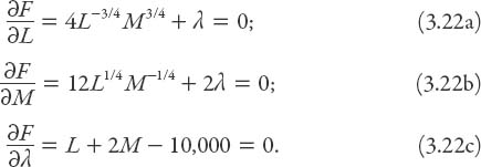
From equations (3.22a) and (3.22b) we eliminate λ to find that M = 3L/2. From (3.22c) it follows that M = 2500, and hence that L = 3750. Finally, from (3.22a), λ = −4(2500)^−3/4 (3750)^3/4 ≈ −5.4216, so the unique critical point of F is (2500, 3750, −5.4216). The maximum value is Q(L, M) = 16(2500)^1/4 (3750)^3/4 ≈ 54,200 sections of fencing.

Question: Can we be certain that this is the maximum value of Q?

Exercise: Show that had we not simplified the constraint equation (3.20), the value for λ would have been λ ≈ −0.1084 but the maximum value of Q would remain the same.

X = A_n: A MORTGAGE IN THE CITY

The home has been built; now it’s time to start paying for it. It’s been said that if you think no one cares whether you’re alive or not, try missing a couple of house payments. Anyway, let’s set up the relevant difference equation and its solution. It is called a difference equation (as opposed to a differential equation) because it describes discrete payments (as opposed to continuous ones).

Suppose that you have borrowed (or currently owe) an amount of money A₀, and the annual interest (assumed constant) is 100I % per year (e.g., if I = 0.06, the annual interest is 6%), compounded m times per year. If you pay off an amount b each compounding period (or due date), the governing first-order nonhomogeneous difference equation is readily seen to be

The solution is

Let’s see how to construct this solution using the idea of a fixed point (or equilibrium value). Simply put, a fixed point in this context is one for which A_n+1 = A_n. From equation (3.23) such a fixed point (call it L) certainly exists: L = Bm/I. If we now define a_n = A_n − L, then it follows from equation (3.24) that

that is

Thus we have reduced the nonhomogeneous difference equation (3.23) to a homogeneous one. Since a₁ = λa₀, a₂ = λa₁ = λ²a₀, a₃ = λa₂ = λ³a₀, etc., it is clear that equation (3.25) has a solution of the form a_n = λⁿa₀. On reverting to the original variable A_n and substituting for L and λ the solution (3.24) is recovered immediately.

Exercise: Verify the solution (3.24) by direct substitution into (3.23).

Here is a natural question to ask: How long will it be before we pay off the mortgage? The answer to this is found by determining the number of pay periods n that are left (to the nearest preceding integer; there will generally be a remainder to pay off directly). The time (in years) to pay off the loan is just n/m (usually m = 12 of course). To find it, we set A_n = 0 and solve for n. Thus

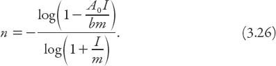
Exercise: Verify this result. And use it to find out when you will have paid off your mortgage!