Testing and statistical quality control in textile manufacturing
Abstract:
This chapter discusses the use of statistical tools, such as measurement of variability, differences between means, significance of variables, control charts and hypothesis testing in textile industries. It is necessary to test the fibre, yarn and fabric for their quality while purchasing in bulk in the industry. An entire batch cannot be accepted by testing only one or two samples. Acceptance sampling technique is a reliable method of selection of samples from bulk. The quality of the product or process can be identified by control charts. Certain controllable variables such as count of yarn, strength, etc. are taken for analysis and their importance is found by statistical significance tests. So in this chapter, different statistical techniques and their applications in textile industry are clearly explained with relevant examples.
3.1 Introduction: statistical quality control
The modern textile industry is a complex, high technology industry facing numerous competitive challenges. Markets are becoming more complex. Short life cycles are common, and demands for rapid response and justin-time delivery are growing. As competition continues to increase, textile companies must rely more on superior quality, innovative products and rapid response to customer needs, to secure markets and continue to grow. To cope with these challenges, many textile companies have implemented quality management initiatives, to reduce costs and increase both product quality and customer satisfaction.
One of the most recent trends in automation is the use of continuous monitoring systems for on-line quality measurement and for recording defects. The continuous monitoring of a process often produces more data than manufacturers are equipped to use profitably, and continuous correction of a process based on a data stream may actually decrease product quality or mask problems needing attention.
Statistical quality control (SQC) is designed to sample a large population on an infrequent basis. Quality assessment therefore only takes place on a small portion of the total product. It has been argued that the use of continuous monitoring would mean that there would be no need for SQC. This attitude assumes that the sole function of SQC is to catch the defective product before it reaches the customer (i.e. acceptance sampling), and ignores the potential for statistics as a tool for product improvement. In recent years, those SQC techniques that worked well for final product quality control have been applied to both the materials being processed and to process conditions. This procedure is now known as statistical process control (SPC). However, some SPC techniques that work with infrequent sampling may not be useful when very frequent or continuous sampling is necessary. Nevertheless, SPC is currently widely used in the textile industry.
3.2 Basic measurement concepts in statistical quality control
SQC comprises the set of statistical tools used by quality control professionals. It can be divided into three broad categories:
i. Descriptive statistics: These are used to describe quality characteristics and relationships. This group includes the mean, standard deviation, range and distribution of data.
ii. SPC: This involves inspecting a random sample of the output from a process and deciding whether the characteristics of the products in the sample fall within a predetermined range. SPC is used to determine whether the process is functioning properly or not.
iii. Acceptance sampling: This involves random inspection of a sample of goods. Based on the results of the sample, a decision is made as to whether a batch of goods should be accepted or rejected.
The tools in each of these categories provide different types of information for use in quality analysis. Descriptive statistics are used to describe certain quality characteristics, such as the central tendency and variability of observed data. Although descriptions of specific characteristics are helpful, they are not enough to identify whether there is a problem with quality. Acceptance sampling can help to solve this problem. However, although acceptance sampling is helpful in deciding on acceptability after the product has been produced, it does not aid in identifying a quality problem during the production process. To do this it is necessary to use tools from the SPC category.
Variation in the quality of manufactured textiles is inevitable. The manufacturing processes currently in use are not capable of producing completely identical products. However, inspection of all of the raw materials and finished goods is impossible, because:
• The standard test is destructive in nature. For example, a fabric manufacturer buys yarn from a spinning mill. It has been settled between the two parties that each consignment of yarn delivered to the fabric manufacturer should have an average linear density inside the tolerance range 40 ± 1 Tex. When the batch of yarn is delivered, it would be impractical to test the whole consignment for whether or not the average linear density lies within the tolerances, as the standard test for linear density is destructive. There would therefore be no product left to work with.
• The population size is too large. For example, a menswear manufacturer marks the size of the trousers he produces according to the waist size. In order to design the trousers, therefore, he must know the average waist size of the men in the population to whom he is hoping to sell the trousers. To determine this average exactly, the waist size of every man in the population would have to be measured, which would of course be prohibitively expensive and time-consuming.
• The rate of production is too high to examine every product. For example, a garment manufacturer knows from past experience that usually 2% of the garment blanks he produces are defective. He is content with this level of defective items but he does not want it to increase, so he aims to control the level, that is, to detect quickly any increase in the number of defective items being produced so that remedial action can be taken. To do this, garment blanks must be inspected, but the rate of production is too high to examine every single blank.
The only reasonable method of addressing the above problems is to examine a small fraction of the population or output, on the assumption that the results of the sample are representative of the untested population or output.
However, there are still some questions that arise, for example:
• Using sample data, what can be said about the average value of the population from which the sample was drawn?
• How many standard tests should be carried out?
• How should the test results be used to describe whether or not the population meets the required specifications?
• How should these results be used to detect a change in the preset levels?
When there is variation within a population and only a sample has been examined, our knowledge of the population is incomplete and uncertain. Statistical methods deal with this by also measuring the degree of uncertainty.
The statistics can be summarised according to the data:
3.2.1 Measures of central tendency
Central tendency represents the average of set of values or data. The average is the general term which can be specifically defined by three different terminologies namely, mean, median and mode.
Arithmetic mean
This is a commonly used term in the industry that has the advantages of (1) being simple to understand, (2) being easy to calculate, and (3) using all the measurements. It is therefore the most popular method used to locate a distribution.
where Xi = observed value, n = sample size, N = population size.
Median
This is the middle value when the data are arranged in increasing or decreasing order. The median divides the area under the frequency curve into two equal parts.
where L is the lower limit of the median class, f is the frequency of the median class, h is the class interval, C is the cumulative frequency of class preceding the median class.
Example:
Suppose 15 threads have been tested for single thread strength in grams and the values have been noted down in order of increasing strength:
The median is the eighth value, that is, 187 g.
Should there be an even number of values, then the mean of the two middle values is taken to determine the median:
The median is the sum of the fifth and sixth values divided by 2, that is (152 + 153) ÷ 2 = 152.5 g.
Mode
The mode is the value occurring most frequently in the data.
where L is the lower limit of the modal class, f1 is the frequency of the modal class, f0 is the frequency of class preceding the modal class, f2 is the frequency of class preceding the modal class, h is the class interval.
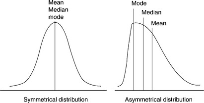
The median and the mode are not usually used in the textile industry. If the frequency curve is symmetrical the mean, median and mode will coincide. Where the curve is moderately asymmetrical, there is an interesting approximate relationship between the three values (Fig. 3.1):
3.2.2 Measures of variation
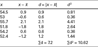
As an example, the deviations for the sample of garment blank lengths are given in Table 3.1. From Table 3.1, sample variance for the garment blank length is found as S2 = 10.62/(6–1) = 2.124 cm2
Since S2 = 2.124 cm2, we find that the standard deviation of the garment blank length data is S = (2.124)1/2 = 1.46.
For the garment length data, ![]() and s = 1.46 cm, so the coefficient of variation is C = 100 × 1.46/53.6 = 2.72%
and s = 1.46 cm, so the coefficient of variation is C = 100 × 1.46/53.6 = 2.72%
Example:
Of a large batch of hand towels, 5% are under 60 g in weight and 40% are between 60 and 65 g. Assuming the normal distribution, find the mean weight and standard deviation.
Solution: If we consider the normal distribution of variant X, that is, mass of hand towel:
The area that will lie to the left of X = 60 is 0.05The area between z = 0 and ![]() is 0.50 – 0.05 = 0.45
is 0.50 – 0.05 = 0.45
From the table, the value of z1 corresponding to this area is 1.645.Therefore,
Also, the mass of 40% of the hand towels is between 60 and 65 g, the area between the ordinates at X = 60 and X = 65 is 0.4 or the area to the left of the ordinate at X – 65 is 0.45. The area between z = 0 and ![]() is 0.50 – 0.45 = 0.05. The value of z2 corresponding to this area is 0.13.
is 0.50 – 0.45 = 0.05. The value of z2 corresponding to this area is 0.13.
Solving equations (i) and (ii):
Result: σ = 3.3 and ![]() .
.
Statistical techniques are important tools for effective process control and innovative solutions to problems. The main focus of statistical techniques is to avoid defects that are produced in the manufacturing process. Experiments designed to assess the advantages of novel types of processing or to determine optimal conditions also fall into the category of SQC. Statistical techniques are also very useful in determining sample size, deciding rate of recurrence of inspection, deciding natural limits of variation of the process, testing conformity of sample to specification provided and so on.
In any product line, no two articles are perfectly identical. For example, it is impossible to find two bundles of yarn with exactly the same count, strength, evenness, length, etc. This is due to raw material variation. The product quality depends on the raw materials used in the process and the level of technical enhancement attained during manufacturing. Machines and tools will sustain wear and tear through use and it is neither practical nor cost-effective to remove or repair the machines after every small occurrence. Therefore, a certain margin for error must be built into the manufacturing process.
3.2.3 Sampling error
It is worth noting that there is room for variation in the accuracy of samples. For example, although the average count spun by a mill can be determined as 40sNe, the count in individual leas could fall anywhere between 35sNe and 45sNe in 95% of the leas produced. The higher the number of samples tested, the closer the average sample count comes to the actual count spun by the mills. The disparity between the actual count (40) and the count estimated from the sample (35–45 assuming the sample size is one lea), is termed the ‘standard error’ due to sampling.
The standard error in the estimated count from a sample of ‘n’ is given by ![]() at 95% confidence limits.
at 95% confidence limits.
It is important to consider the sampling error while interpreting any computed data. For example, for a CV of 4.5%, if the average count of a sample of 36 leas is 60 then the count for the department as a whole would be, at 95% confidence, within
3.3 Interpretations: critical difference
With the advent of a large number of testing instruments, it has become possible to test various aspects of the quality of textile materials and therefore present a large volume of data to the manager for decision-making.
However, interpretation of the test data is made more complex due to the instrumental and sampling errors associated with the data, as discussed above. Experimental work has been carried out by research associations to assess the variability of each property of fibre and yarn and to fix the levels of variability in average values, which manufacturers could then accept as a base while dealing with test data. This variability has been expressed in terms of critical difference. With help of such values the test data can be interpreted meaningfully.
Critical difference (CD) is a measure of the difference between two values that arises solely due to natural or unavoidable causes. When the difference between two values exceeds the CD, then the two values are said to be statistically different. The CD depends upon the CV% and the number of tests carried out to determine the quality characteristics.
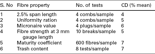
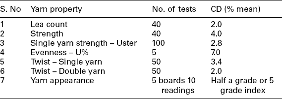
The values of CD for various fibre and yarn properties are given in Tables 3.2 and 3.3. These values are based on the recommended number of tests for each fibre or yarn property as given in the same labels. If, however, the number of tests carried out to determine a specific property differs from the recommended number, then the CD would vary from the values reported. Under such circumstances, a new CD must be computed using the formula:
where N1 = number of tests recommended in Tables 3.2 and 3.3, N2 = number of tests actually conducted.
i. an increase in CV% would increase CD and
ii. an increase in the number of tests (N2) would decrease CD.
3.3.1 Fibre test data
In the following section some of the major problems encountered commonly in the mills are discussed and solutions are suggested.
Consistency between basic and delivery samples
A mill has received a basic sample of Shankar-6 cotton, whose micronaire value on testing was found to be 4.0. The delivery sample had a micronaire value of 3.8. The mill manager is interested to know whether they could accept the delivery sample. Four tests were carried out on both the basic and delivery samples to determine the micronaire value.
The extent of variation present between the two samples is computed as follows:
Since the actual difference of 5.13% is less than the CD of 6%, the delivery sample could be considered as not significantly different to the basic sample, as far as the micronaire value is concerned. The mill manager could therefore accept the delivery sample.
In above example, the CD is computed based on the mean of the micronaire values of the basic and delivery samples. This is because when two samples are compared to determine their difference, the allowable limits for the CD should be fixed based on the average of the two samples.
However, if data from a test is to be compared with a specific value, a different procedure should be adopted, as shown in the example below.
A mill wants to purchase cotton of 3.7 micronaire value to spin 60s count. The cotton sample received from a supplier was tested for micronaire and it was found to be 4.0 (on the basis of four tests). The mill technician now needs to know whether the cotton sample conforms to his requirements or not.
Difference in micronaire values between the specific value (3.7) and the actual value (4.0) = 4.0 – 3.7 = 0.3
Since the mean value is being compared with a specific value, the CD should be calculated on the basis of the specific value.
The CD for micronaire value (as in Table 3.2) = 6%
Since the actual difference of 8.1% is higher than the CD of 6%, the mill could not purchase cotton from that supplier. In the same way, data on the fibre length, strength, fineness, maturity and trash could be analysed with the proper use of the CD values reported in Table 3.2.
3.3.2 Yarn test data
The following sections cover some of the common problems and their respective solutions in the spinning division of most of the mills.
Pinion changes in spinning frame
Mill ‘D’ spins 60s Ne using a specific variety of cotton. A random sample of 40 cops is taken from a spinning frame and the count is checked by taking one lea from each cop. The average count is found to be 62s Ne. The problem is to ascertain whether changing the draft wheel in the spinning frame is necessary to correct the count. (The change wheel in the frame has 50 teeth.)Difference between actual and nominal count = 62 – 60 = 2
For reasons explained earlier, the percentage difference is calculated on the basis of the nominal count.Thus the difference expressed as a percentage of the nominal count = (2/60) × 100 = 3.3%
Since the difference of 3.3% is greater than the CD value of 2% (Table 3.3), the count of yarn from the particular spinning frame (62s Ne) is significantly different from the nominal count (60s Ne).
But while making wheel changes to correct the count, the limitation imposed by mechanical factors should also be taken into account. A change of pinion is advantageous only when the true deviation from the desired count exceeds C/2A, where C is the nominal count and A is the number of teeth in the change pinion.
Since the actual difference of 3.3% is greater than the sum of the CD and mechanical errors (2% + 1%), wheel changes could be recommended in the spinning frame to correct the count.
Yarn evenness between samples
Mill ‘E’ produces 40s yarn. While testing two samples from different spinning frames for evenness, the U% values are found to be 13.8 and 15.0 respectively on the basis of ten observations in each case. It is then necessary to assess whether the yarn produced in the frames is even or not.
Because ten tests were done to assess U%, the CD of 7% given in Table 3.3 needs correction.
Using formula [3.1]
The difference between the two samples expressed as a percentage of the average = (1.2/14.4) × 100 = 8.3%
Since the actual difference of 8.3% is higher than the CD of 5%, it can be concluded that the two yarn samples are not even.
Average and minimum CSP
Mill ‘F’ produces 50s P/V yarn for the export market. The mill intends to produce yarn with a minimum CSP of 2500 and CV strength of 6%. The mill would like to decide the average CSP it has to achieve so that the minimum CSP is 2500.
The relationship between the average and minimum CSP is given by the formula:
Thus, if the mill aims at an average CSP of 3049 with a CV of strength not greater than 6.0%, then it can expect to produce a yarn with a minimum CSP of 2500.
3.4 Interpretations: ‘t’ tests, ‘F’ tests and the chi-square method
The following section covers the tests for analyzing the statistical significance of the data set, namely, the ‘t’ test, ‘F’ test and chi-square method.
3.4.1 ‘t’ and ‘F’ tests
To analyse properties for which CD values are not stipulated, for example, hairiness or CV of twist, special tests need to be applied.
i. ‘t’ test: to compare two mean values,
ii. ‘F’ test: to compare two variances (square of standard deviation).
Hairiness between samples
A mill produces 80s P/C yarn. While testing two yarn samples for hairiness, one each from the RF1 and RF2 ring frames, the number of hairs per 1000 m are found to be 8000 and 10 000. The CVs of hairiness are therefore 30% and 40% respectively (on the basis of 20 tests for each sample). The mill wants to know whether the RF2 ring frame is producing a more hairy yarn.
In order to decide whether the two samples differ in terms of hairiness, the ‘t’ value of significance is to be applied as no CD value for hairiness is reported.
where X1 = average hairiness of sample 1, X2 = average hairiness of sample 2, n = number of tests carries out for sample 1 and sample 2, S1 and S2 = standard deviations for sample 1 and sample 2, respectively.
From the value of CV and mean, the SD values can be deduced. Thus, S1 = 2400 and S2 = 4000
The calculated value of ‘t’ should then be compared against the standard value of ‘t’, which is available in any standard statistics book. For this, it is necessary to know the degrees of freedom in the problem concerned. The degree of freedom is 2(n – 1), where ‘n’ is the number of tests carried out for samples 1 and 2.
The value of ‘t’ for 38 degrees of freedom is 2.0.
Since the calculated value, 1.9, is less than 2.0, it can be concluded that the yarns from both frames are similar with regard to hairiness.
Twist variability among samples
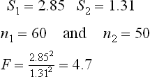
Mill ‘H’ produces 40s yarn. On testing two samples drawn from two spindles for twist, the standard deviations of twist were found to be 1.31 and 2.85 based on 50 and 60 tests respectively. The mill therefore wants to find out whether the two samples differ in terms of their twist variation.
As two standard deviations are to be compared, the ‘F’ test needs to be conducted, as follows:
S1 = standard deviation of twist for one sample (sample 1) for which the number of tests conducted is n1;
S2 = standard deviation of twist for the other sample (sample 2) for which the number of tests conducted is n2.
S1 and S2 are to be chosen in such a manner that ‘F’ is always greater than 1. In the present problem,
The value of F (refer to the ‘F’ table in any standard statistics book, for df1 = 59 and df2 = 49) is 1.6 where df1 = degrees of freedom for sample 1 and df2 = degrees of freedom for sample 2.
Since the calculated value of F (4.7) is greater than the 1.6, it is confirmed that the two yarns differ significantly in their twist variability.
Application of ‘F’ test: auto levellers in cards
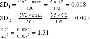
Due to the incorporation of auto levellers in the high production cards in a mill, the CV% of card sliver decreased from 4 to 3.5. It is now necessary to determine whether this difference is statistically significant. The mean value of a hank of card sliver is 0.2.40 readings were taken to measure CV%.
As two CV values are to be compared, the ‘F’ test must be employed:
This value is to be compared with the values of ‘F’ in statistical tables. Since 40 readings were taken to assess CV%, the degrees of freedom are:
The value of F (for n1 = 39 and n2 = 39) = 1.53Since the calculated value of ‘F’ (1.31) is lower than that given in tables (1.53), it can be inferred that auto levellers do not improve the CV% of card sliver.
3.4.2 The χ2 (chi-square) method
This method is used when there is no prior knowledge of the distribution of the test values.
where O and E are observed and expected values, respectively.
Comparison of end breaks
A mill maintains an average end breakage rate of 150 breaks per 1000 spindle hours in 60s Ne. When the mixing was changed, the breakage rate increased to 220 breaks per 100 spindle hours. In order to determine whether the change of mixing increased the breakage rate, the following can be used (breaks were observed for 1000 spindle hours):In the present problem O = 220 and E = 150
The χ2 (chi-square) value (refer to the ‘χ2’ table in any standard statistics book) for 1 degree of freedom is 3.84.Since the actual value of χ2 (32.7) is greater than 3.84, it could be concluded that the end breaks did increase due to the change in mixing.
Comparison of neps during carding
A mill processes cotton fibre through a card-A and card-B. Neps in the card web were assessed by taking ten readings from each of the cards. The neps were found to be 120 and 80 per 10 g respectively. The mill now needs to find out whether the card-A really does generate more neps.
We have here two observed values for neps (120 and 80) but the expected number of neps from each card is unknown. Under the circumstances, an assumption is made that the expected value is the mean of the two observed values, and the following formula is used:
where A and B are the two observed values.
χ2 (chi-square) value for 1 degree of freedom = 3.84.Since the actual value of χ2 (8) is greater than 3.84, it is confirmed that the card-A generates more neps.
3.5 Decision-making using control charts
Process control forms a key part of the overall effort to maintain quality in yarn manufacture. The properties of the material as determined at different stages of processing act as indicators to ascertain whether a correction at any specific stage of processing is necessary or not. The application of appropriate statistical methods would facilitate a proper understanding of the data. SPC methods extend the use of descriptive statistics to monitor the quality of the product and process. They can be used to determine the amount of variation that is common or normal and to monitor the production process to make sure production stays within this normal range; that is, that the process is in a state of control. The most commonly used tool for monitoring the production process is a control chart. Different types of control charts are used to monitor different aspects of the production process.
A control chart (also called a process chart or quality control chart) is a graph that shows whether a sample of data falls within the common or normal range of variation. A control chart has upper and lower control limits that separate common from assignable causes of variation. A process is defined as out of control when a plot of data reveals that one or more samples fall outside the control limits.
Control charts are one of the most commonly used tools in SPC. They can be used to measure any characteristic of a product, such as the count or hank, strength, U%, etc. The different characteristics that can be measured by control charts can be divided into two groups: variables and attributes.
Variable data are data that can be measured on a continuous scale such as a thermometer, a weighing scale or a tape rule.
Attribute data are data that are counted as having a certain attribute or value; for example, as good or defective, or as possessing or not possessing a particular characteristic.
3.5.1  and R charts
![]() and R charts are control charts that are commonly used to control average (
and R charts are control charts that are commonly used to control average (![]() ) and variation – range (R) in terms of data. They are used to control the hank or count of textile material, strength, U%, etc. The method for creating these charts is given below:
) and variation – range (R) in terms of data. They are used to control the hank or count of textile material, strength, U%, etc. The method for creating these charts is given below:
a. Collect data over a fixed period of time, testing 20 to 25 samples per day in sub-groups of 4 to 5.
b. Calculate the average (![]() ) and range (
) and range (![]() ) the range for each sub-group, followed by the overall average.
) the range for each sub-group, followed by the overall average.
c. Calculate the upper and lower limits of the group ranges: ![]() and
and ![]() , where D4 and D3 are factors that can be read from the statistical tables.
, where D4 and D3 are factors that can be read from the statistical tables.
d. If any group range is higher than ![]() or lower than
or lower than ![]() omit these values and recalculate the
omit these values and recalculate the ![]() and the upper and lower limits. Repeat this procedure until all the group ranges fall within the limits.
and the upper and lower limits. Repeat this procedure until all the group ranges fall within the limits.
e. The control limits to be fixed for the averages are ![]() The A2 values can be found in any standard statistical book.
The A2 values can be found in any standard statistical book.
f. Plot the centre line and control limits, then add the sample number and data to the X-axis as well as the average and range to the Y-axis.
After setting up the charts for ![]()
![]() and
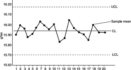
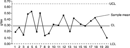
and ![]() the daily test values should be plotted in the chart as and when the tests are carried out. Figures 3.2 and 3.3 provide examples of
the daily test values should be plotted in the chart as and when the tests are carried out. Figures 3.2 and 3.3 provide examples of ![]()
![]() and
and ![]() charts.
charts.
3.5.2 Using p and C charts
The p chart is used to record the fraction of defectives; that is, the proportion of excessively high or low weight laps or machine stoppage. The C chart is used to record the average number of defects. The control limits are as follow:
where p is the average fraction of defectives; and
where c is the average number of defects per unit.The method of calculating average values and fixing control limits is the same as described above for the ![]() -bar and
-bar and ![]() -bar charts.
-bar charts.
Example for p chart
In a blow room situation, for the average lap weight to be under control, the proportion of heavy laps should be 0.5. If 100 laps are produced in one shift, then the control limits for the proportion of heavy laps would be
If the proportion of heavy laps lies between 35% and 65%, then the lap weight is under control.
3.6 Decision-making: hypothesis testing
A statistical hypothesis is an assumption about a population parameter that may or may not be true. In order to determine whether or not it is true, the most accurate method would be to examine the whole population. However, this is usually impractical, so a random sample needs to be generated and used as a representation of the whole population. The sample is then examined to determine whether it is consistent with the statistical hypothesis. If it is not, then the hypothesis is considered to be untrue.
There are two types of statistical hypothesis; the null hypothesis (H0), which states that the observations made from two samples are due to chance; and the alternative hypothesis (H1 or Ha), which suggests that the observations from the samples are influenced by a non-random cause.
3.6.1 Hypothesis tests
The decision to accept or reject a null hypothesis is described as hypothesis testing. It consists of four steps:
3.6.2 Decision errors
A hypothesis test can result in two different types of error. A Type 1 error occurs when the researcher rejects a null hypothesis that then turns out to be true. The probability of this occurring is called the ‘significance level’ and is denoted by α. A Type 2 error occurs when the researcher accepts a null hypothesis that then turns out to be false. The probability of this occurring is called the ‘power’ and is denoted by β.
3.6.3 Decision rules
Decision rules are included in the analysis plan, and are used to determine whether to reject the null hypothesis. Statisticians describe these rules with reference to either a P-value or a region of acceptance. A P-value measures the strength of the evidence in support of a null hypothesis (e.g. the probability of observing the test statistic assuming the null hypothesis is true); whereas the region of acceptance is a range of values into which the test statistic must fall if the null hypothesis is to be accepted. The region outside the region of acceptance is called the region of rejection. If the test statistic falls into this region, it is said that the hypothesis has been rejected at a level of significance. Where there is only one region of rejection (e.g. on one side of the sampling distribution), the test of the hypothesis is referred to as a ‘one-tailed’ test. Where the region of rejection occurs on both sides of the sampling distribution, the test is referred to as ‘two-tailed’.
3.7 Decision-making: significance testing
Significance testing is used to determine whether there is enough evidence to reject the null hypothesis; that is, if the difference between the assumed value in the null hypothesis and the observed value in the experiment is large enough to reject the possibility of the result being due to chance. The ‘significance level’ is the value used to specify how large the difference has to be in order to reject the null hypothesis. This is usually 1% or 5%. The other 99% or 95% is described as the ‘confidence level’.
3.7.1 Test for a single mean (large sample available)
This is performed in situations in which a significance test for a single mean is appropriate. In these cases, the researcher conducting the experiment has to decide between two possibilities: either the mean = μ0, or it has not changed. See Example 1.
3.7.2 Test for a single mean (small sample available)
The significance test described in the previous section is suitable for use in two different cases: when the value of standard deviation (σ) is already known, and when the sample is sufficiently large to enable a good estimate ‘s’ of σ to be drawn. The latter condition is generally encountered when the sample size is greater than approximately 30.
When the sample size is smaller than this, the sample estimate ‘s’ may not be precise enough, meaning that some corrections will have to be made to take into account potential errors in the calculation of a that may occur due to the use of ‘s’ instead of σ.
The modification to the test is simple and straightforward. It is necessary to consult the t-table rather than the normal distribution tables in this case.
The following calculation should be made:
and the observed value compared with the tabulated values for k = n – 1 degrees of freedom.See Example 2.
3.7.3 Test for the difference between two means (independent samples)
Suppose there are two populations, both with unknown mean μ1 and ;μ2, and it is necessary to test the null hypothesis that their difference is equal to a specified value μs. Many practical situations involve the testing of equality of means, that is, μs = 0, but any other value can also be specified. The alternative hypothesis could be either single sided or double sided.
Independent samples of size n1 and n2 are taken, randomly chosen from the two populations, the means of which are ![]() and
and ![]() . Therefore
. Therefore ![]() is a point estimate of the difference μ1 – μ2.
is a point estimate of the difference μ1 – μ2.
The value of α can be found by computing:
and comparing the resulting value with normal distribution tables. But this calculation requires knowledge of the unknown population variances σ12 − σ22. If the samples are reasonably large, that is, n1 and n2 are greater than approximately 30, then σ12 and σ22 may be replaced by their sample estimates s12 and s22. The equation then becomes:
When this equation has been used to obtain U, the value of α can be found from the standard tables.
However, sample sizes are usually small, that is, less than 30. In this situation, the above methodology can lead to errors in the significance level. It is therefore necessary to assume two things in such cases: one, that the two populations are normal; and two, that their variances are equal.
Here, the common variance is given by the equation:
which is used to calculate:
Therefore in this case, k = n1 + n2 – 2 degrees of freedom.
3.7.4 Test for the difference between two means (matched samples)
If the samples available for the tests are not chosen independently from the populations of which the means are being compared, that is, the samples are matched in pairs, then a different method is used.
3.7.4 Test for single variance
If the results of inspection of a sample set reveal a high level of variability among the sample units, the manufacturer or user may call for some change in the manufacturing process of the item on which the tests were carried out. Following the alterations, the manufacturer or user will obviously wish to check whether or not the changes introduced in the process parameters have resulted in some reduction in the variability of the sample items or not. In such a case, the variance of the new sample set is compared with a preset or standard variance value that falls within the acceptable range.
3.7.6 Test for difference between two variances
Following a modification to the process as described in the previous example, it may sometimes be necessary to compare the variability of two sample sets and not the variance of the new sample set from any preset standard. In such a case, the variances of two sample sets, one taken before the modifications in process and the other taken after the modifications, are compared. The results will show whether there has been a significant reduction in variability; that is, whether the process modifications have had a positive result or not.
3.7.7 Test for a single proportion
Variation is inherent to all textile products. It is common practice to set norms or specifications for the end product in a manufacturing process; however it is never possible to ensure that all products have exactly the same dimensions or characteristics. Some proportion of the bulk production is bound to be defective in some way or other. Therefore, an acceptable level of defective items in a specific amount of bulk is always preset, on the basis of which it can be assumed prior to any manufacturing process that x% of the products will probably be defective. But in some cases, the proportion of defective items from a manufacturing cycle is substantially more than x%. It is then necessary to carry out a further test to conclude whether the process has in fact developed a fault.
Examples
Example 1: Single mean with a large sample (n greater than 30)
One hundred ring bobbins are tested for count and the mean count is found to be 34.2 s. The frame should be spinning 34 s. If the standard deviation of the sample is 0.62, can we conclude that the frame is really spinning off count?
Answer
Step 1: Calculate the standard error of the mean by using the standard deviation of the sample as an approximation of the SD of the population:
Step 2: Calculate the difference between the nominal mean and the sample mean and divide by SE.
Step 3: Compare the value obtained from step 2 with the values 1.96 and 2.58:
Conclusion: The difference in count is statistically significant at the 1% level. The frame is spinning ‘off count’.
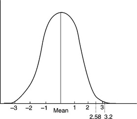
To reach a conclusion we have noted that the value 3.2 is greater than 2.58. This value (3.2) represents the difference between the nominal and sample means expressed in terms of the standard error.
A glance at Fig. 3.4 will show that the chance of the sample mean lying outside the limit (nominal mean ± 2.58 SE) is only one in 100 if the population from which the sample was drawn had a mean equal to the nominal mean. Once it has been concluded that there is a real difference, the ring frame should be adjusted. The chance of this conclusion being incorrect is only 1 in 100.
Example 2: Single mean with a small sample
Twelve ring cops were tested for count and the mean was found to be 94.2s. The standard deviation of the twelve results is 2.2 counts. If the nominal count is 92s, then the ring spinning process is too fine.
Answer
Step 1: Estimate the standard error of the mean by dividing the standard deviation of the sample by the square root of the number in the sample.
Step 2: Calculate the value of t:
Step 3: Consult the t-table for v = n – 1, then compare the value of t obtained in step 2 with the 5% and 1% values for t.
Conclusion: Since 3.47 is greater than 3.106, we can conclude that the ring is spinning too fine because the difference between the sample mean and the nominal mean is significant at the 1% level.
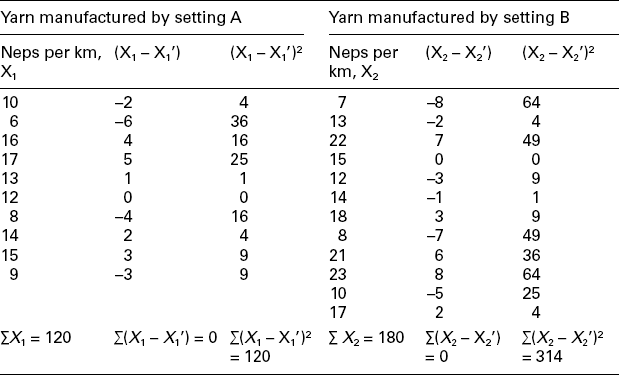
Example 3: For 10 randomly chosen samples of yarn, manufactured by two different card settings, the effect on neps per 1000 km is as follows:
Setting B: 7, 13, 22, 15, 12, 14, 18, 8, 21, 23, 10, 17
It is necessary to test whether card settings A and B differ significantly in their effect on neps per km.
Solution: Let us take the null hypothesis that A and B do not differ significantly with regards to their effect on neps per km.
Calculating the required values:
Mean neps per km value with setting A
Mean neps per km value with setting B
Putting values in equation (i),
Degree of freedom, v = n1 + n2 – 2 = 10 + 12–2 = 20.
For v = 20, the table value of t at 5% level is 2.09. The calculated value is less than the table value and hence the experiment provides no evidence against the hypothesis. It can therefore be concluded that there is no significant difference between the two card settings as regards their effect on the value of neps per km.
Table 3.5
Weight of cones and variability after conditioning under two different process conditions: A and B
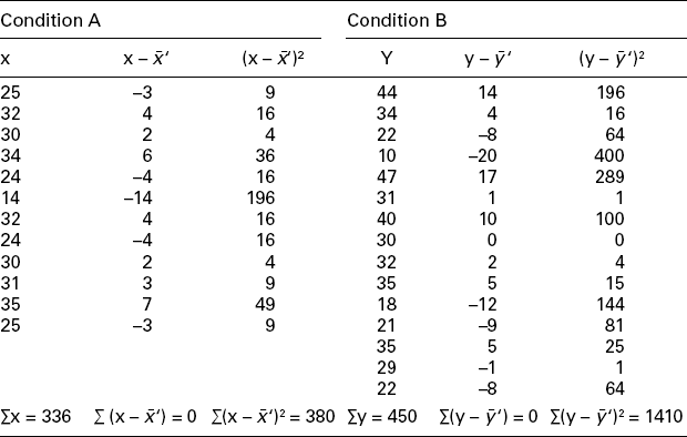
Example 4: Below are listed the weight gains (in g) of cones after conditioning, when processed under two different process conditions: A and B:
Condition B: 44, 34, 22, 10, 47, 31, 40, 30, 32, 35, 18, 21, 35, 29, 22
It is necessary to test whether the two conditions differ significantly as regards their effect on increase in cone weight.
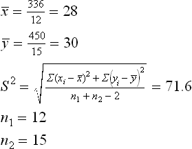
Solution: Null hypothesis, H0: μx = μy; that is, there is no significant difference between the mean increases in weight under conditions A and B.
The alternative hypothesis, H1: MX ≠ MY (two-tailed)
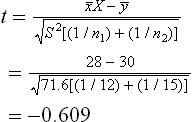
Tabulated t0.05 for (12 + 15–2) = 25 degrees of freedom is 2.06.
Analysis: since the calculated value of t is less than the tabulated value, H0 may be accepted at a 5% level of significance and we may conclude that the two conditioning parameters do not differ significantly as regards their effect on weight gain.
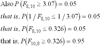
Example 5: A polyester fabric is stitched using two different types of sewing threads: a 100% polyester sewing thread and a polyester-cotton blend sewing thread. Two random samples of 11 and 9 stitched fabrics show the sample standard deviation of the seam strengths as 0.8 and 0.5 respectively. Assuming that the seam strength distribution is normal, it is necessary to test the hypothesis that the true variances are equal at the 10% level. [Assume that P (F10, 8 ≥ 3.35) = 0.05 and P (F8, 10 ≥ 3.07) = 0.05.]
Solution: We want to test the null hypothesis, H0 : σx2 = σy2 against the alternative hypothesis, H1 : σx2 ≠ σy2 (two-tailed).
The following values are given: n1 = 11, n2 = 9, Sx = 0.8, Sy = 0.5.
F = Sx2/Sy2 follows F distribution with (n – 1, n – 2)df
or
Similarly,
Therefore,
The significant values of F for the two-tailed test at the level of significance α = 0.10 are:
and
We are given the tabulated significant values:
Therefore, from a, b and c, the critical values for testing the null hypothesis against the alternative hypothesis at the level of significance α = 0.10 is given by:
Since the calculated value of F (= 2.5) lies between 0.33 and 3.35, it is not significant and so the null hypothesis of the equality of the population variances may be accepted at the level of significance of α = 0.10.
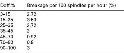
Example 6: The breakages in a ring frame (while spinning 30s) count across the doff are given successively as doff completes. According to mill practice, the breakage percentage for this count is 2%. What should the variance of population be at the acceptable (1%) level of significance?
Solution: Assuming that there is no significant difference in the breakage percentage at various positions of doffs (the null hypothesis):
Sample size, n = 7Because the sample is small, the t-test must be used here.Degree of freedom, v = n – 1 = 7–1 = 6
The tabulated value of t is t0.005, 6 = 3.71The calculated value of t is ![]()
Since the calculated value of t is less than the tabulated value, the null hypothesis is acceptable at a 1% level of significance. There is no significant difference in the breakage percentage at various positions of doff.
Example 7: The waste (in g per batch) found at various speed frames in a spinning unit are as follows:
Do the values vary significantly at a 5% level of significance? Mill practice in this case is that waste produced at a speed frame is generally 21 kg per batch.
Solution: Assume the null hypothesis that there is no significant difference in the waste obtained at various speed frames.
Sample size, n = 10Because the sample is small, we will use the t-test here.Degree of freedom, v = n – 1 = 10–1 = 9 The tabulated value of t is t0.025, 9 = 2.26The calculated value of t is
 ![]()
Since the calculated value of t is less than the tabulated value, therefore null hypothesis is acceptable at 5% level of significance. There is no significant difference in the waste obtained at various speed frames.
3.8 Testing fibre and yarn properties
3.8.1 Fibre properties
Fibre properties are very important and should be considered in each stage of the textile manufacturing process. There are many different fibre properties, of which the following are most important to textile technicians:
fibre length,fibre strength and elongation,fibre fineness,fibre maturity.
Fibre length is one of the most important fibre characteristics, and has an influence on factors such as spinning limit, yarn strength and evenness, and product appearance. It can also influence productivity in textile manufacturing. For example, shorter fibres (e.g. < 4–5 mm) will usually be lost as waste in the manufacturing process. Fibres of 5–15 mm in length tend to contribute to the fullness of the yarn rather than its strength, whereas fibres above 12–15 mm are long enough to contribute to yarn strength and survive carding without significant shortening.
Fibre strength is another important characteristic, with the minimum strength for a useful textile fibre being approximately 6 cN/tex. Fibre bundles are usually tested for strength using HVI instrumentation, which uses the following scale of values:
In most fibres (with the exception of polyester and polypropylene), strength depends on the moisture content, which will change depending on the ambient conditions.
Fibre elongation can be divided into three different categories: permanent elongation, in which the fibre is stretched and does not return to its original shape on relaxation; elastic elongation, in which the fibre does return to its original shape; and breaking elongation, the point at which the fibre breaks. Elongation is measured as a percentage of the original length of the fibre. Elasticity is very important in textile fibres, as textile products must have the ability to return to shape after deformation and stretching, for example, in the elbow of a garment. The fibre elongation should therefore be at least 1–2%. Synthetic fibres often have much higher elongation values, for example, 15–30%, although a very high elongation value can make spinning and drafting more difficult. The relationship between strength and elongation is expressed in a ‘stress-strain’ curve. Each fibre has a typical curve, and it is therefore important when blending fibres that those with similar curves are chosen.
Another of the main fibre characteristics is fineness. The fineness of the fibres in a yarn determines how many fibres appear in a cross-section of the yarn, which in turn determines the strength and evenness of the yarn. There are usually over 100 fibres in yarns used for new spinning technologies, although there can be as few as 30 in yarns for other applications. As well as the yarn strength and evenness, fibre fineness has an influence on the spinning limit and such factors as the drape and lustre of the fabric. The fibre fineness can also influence productivity, in terms of the end breakage rate. Fineness is determined by the relation of mass to length, as follows:
The final fibre characteristic to be discussed in this section is fibre maturity. A natural fibre (e.g. cotton) consists of a cell wall and lumen, and the fibre is said to be more mature as the cell wall thickens. A moisture-swollen cotton fibre is considered ‘mature’ when the cell wall comprises 50–80% of the fibre cross-section; ‘immature’ when it comprises 30–45%; and ‘dead’ when it is less than 25%. It is important that cotton stock does not include too many immature or dead fibres, as these do not have adequate strength or stiffness and so can lead to problems such as loss of yarn strength, variable dye uptake and processing difficulties.
3.8.2 Yarn properties
As well as fibre properties, it is also important to routinely test yarn properties such as fineness/count, twist, strength, evenness and surface integrity.
Yarn fineness can also be described as yarn count, number or size, and as with fibre fineness, can be variable as yarn does not always have a circular cross-section. To address this problem, ‘linear density’ or mass per unit length is used to measure the fineness of yarn. This can be done using direct or indirect systems of measurement. Direct count systems such as the ‘tex’ (Ne) determine yarn count as the mass of a unit in length of yarn, for example, the mass in grams of 1 km of yarn. Other systems such as the ‘kilotex’, which measures mass in kg per kilometre, and the denier, which measures mass in grams of 9000 m, are also used. Indirect count systems determine yarn count as ‘units of length’ per ‘unit of weight’; for example, hanks (840 yards) per pound (lb) or kilometres (km) per kilogram (km).
Yarn twist is the number of spiral turns in a yarn in order to bind the constituent fibres together. Twist is described using three main parameters: direction, level (turns per unit of length) and factor. Twist direction is especially important when twisting two single yarns together to form a ply yarn. The aesthetic and strength requirements of the ply yarn determine whether the twist is Z on Z or S on Z. Forming a ply yarn in this way will result in contraction or extension of the length of the ply yarn compared to the two single yarns, depending on the direction of the twist. This later influences the appearance of the fabric made from the yarn, and can be used for example to create different surface effects. It can also influence the fabric stability or torque.
While linear density is the most practical way to express yarn fineness, as discussed above, it is sometimes necessary to know the yarn diameter, for example, when determining the structural features of a fabric (e.g. width or thickness). The following equations can be used to express the yarn radius as a function of the yarn density:Direct count (tex):
Indirect count (cotton count): 1
The value of the yarn diameter therefore depends on both the linear and volumetric densities of the yarn.
One of the main characteristics of yarn quality is its strength, and there have been many studies devoted to this subject. It is an important parameter throughout textile manufacture; for example, a weak yarn can cause defects and even breakages in spinning and weaving, and processes such as dyeing and sizing can alter the strength and mechanical behaviour of yarn. It is therefore very important to determine and test yarn strength at regular intervals. The stress–strain behaviour of yarn has a direct effect on the properties of the end fabric; for example, a strong yarn will produce a strong fabric.
Finally, testing yarn density is an important factor in textile manufacture. Yarn consists of fibres and air pockets and the packing fraction (φ), which determines the yarn bulk density, is calculated as follows:
Vf = volume of fibres in yarn and Vy = volume of yarn (fibres + air).
The packing fraction indicates the air to fibre ratio; for example, a packing fraction of 0.5 means that there are equal amounts of air and fibre in the yarn (most spun yarns have a packing fraction of well above 0.5). The yarn density again has a direct effect on the properties of the end fabric, as a high packing fraction can create a stiff, weak yarn, whereas a low packing fraction can create a yarn with minimal surface integrity (i.e. it is likely to disintegrate during processing). Yarn density also has an effect on fabric performance, in terms of properties such as flexibility, dimensional stability, strength, insulation and absorption.
The type of fibre used in the yarn and the spinning technique (e.g. ring-spun vs. rotor-spun) can also have an effect on the yarn density.
3.9 Testing fabric properties
It is important to test fabric properties throughout the production process, as part of quality control. Testing the fabric properties at regular intervals ensures that they are suitable for their intended purpose. The following are a few of the important fabric properties that need to be checked regularly:
fabric weight,fabric thickness,fabric strength,fabric abrasion resistance.
3.9.1 Fabric weight
Fabric weight is expressed as the weight of the fabric in grams per m2. It has no limits but does affect the many of the fabric properties.
Fabric weight is a fundamental property that needs to be controlled during the manufacturing process in order to avoid economic loss, for example, by buying heavier fabric than is necessary for the product being manufactured.
Fabric weight, that is, GSM, influences other fabric properties such as thickness, flexural rigidity, bending rigidity, drape, air permeability and thermal properties. For example, the lighter the fabric, the lower its bending rigidity.
3.9.2 Fabric thickness
In order to determine the thickness of a compressible material such as textile fabric, the precise measurement of the distance between two parallel plates should be measured when they are separated by the cloth. A known arbitrary pressure between the plates should be applied and maintained.
It is useful to measure fabric thickness, in order to check the material against the specification.
Fabric thickness is also useful in studying fabric properties such as thermal insulation, resilience, dimensional stability, fabric stiffness, abrasion and total handle value.
Raw material
Fabric construction (Weave: plain weave is stronger than other types, for example floats-twill or satin weave. Density: Low density causes weave slippage which results in seam slippage).
Finish applied to fabric. (For example, a resin finish improves seam slippage.)
Where the fabric is to be subjected to tension (e.g. for industrial purposes), tensile strength is necessary. The tensile strength of a fabric should always be several times greater than the maximum stress likely to be encountered in use, because the strength of most fabrics will diminish during their lifetime due to rubbing, flexing and chemical attack. Fabric tensile strength is also useful in monitoring various relevant process parameters during production. For example, if a shortfall in the fabric tensile properties is observed during production, this observation can help to identify potential causes in the process.
Fabric tear strength
The tear strength of the fabric refers to its resistance to tearing force. Usually fabric tears when it is snagged by a sharp object and the immediate small puncture is converted into a long rip. This is probably the most common type of strength failure, so testing fabric tear strength is very important.
Resistance to tearing force is of great importance in clothing fabrics and in technical fabrics such as those used for parachutes. Tear tests are not suitable for knit fabrics and non-woven fabrics.
It is important to measure tear strength for flat sheet-like materials such as fabric, plastic films, paper and leather. Outdoor clothing and uniforms are examples of clothing where tearing strength is of importance.
Fabric bursting strength
Bursting strength is a method of measuring strength in which the material is stressed in all directions at the same time and is therefore more suitable for materials such as knitted fabrics, lace or non-woven.
Fabrics used in parachutes, filters, sacks and nets are simultaneously stressed in all directions during service. In service, a fabric is more likely to fail by bursting than by a straight tensile fracture; one example is the stress present at the elbows and knees of clothing. During the test, fabric fails across the direction that has the lowest breaking extension.
3.9.4 Fabric abrasion resistance
Abrasion or wear is the wearing away of any part of a material by rubbing against another surface. Textile material becomes unserviceable for several reasons. The first is abrasive wear. Carpets are often discarded because of extensive wear due to abrasive action over a period of time. Measuring the abrasion resistance of fabric is therefore important for customer acceptance and satisfaction, as well as manufacturing practicalities.
The following are factors that can cause abrasion of fabric during usage:
Friction between two fabrics, such as the rubbing of a jacket or coat lining on a shirt, pant pockets against pants fabric, and so on.
Friction between the cloth and external objects such as furniture or seat covers.
Friction between fibres and dust or grit in a fabric, resulting in the fibres being broken or cut. This is an extremely slow process and may take several years before it becomes apparent. It might be observed in home textiles.
The abrasive resistance of a fabric should therefore be tested and controlled, in order to achieve good quality fabrics.
3.10 References
1. Leaf, G.A.V. Practical statistics for the textile industry. Manchester, U.K.: The Textile Institute; 1984.
2. Montgomery, Douglas C., Runger, George C.Applied Statistics and Probability for Engineers. John Wiley & Sons, 2010.
3. Grant, E.L., Leavenworth, R.S. Statistical Quality Control, 6th Ed. New York, USA: McGraw-Hill; 1998.
4. A. Abouelela Radwan, H. Abbas, H. El deeb, S. Nassar, A statistical approach for textile fault detection, IEEE International conference on Systems, Man, and Cybernetics 2000, vol. 4, 2857–2862.
5. Vincent A. Voelz, HypothesisTesting, August 30, 2006, Math Bio Boot Camp 2006, University of California, San Fransisco, pp. 2–11
6. Ratnam, T.V., Chellamani, K.P.Ratnam T.V., Chellamani K.P., eds. Quality Control in Spinning, 3rd Ed, Coimbatore: SITRA, 1999.
7. Booth, J.E. Principles of textile Testing, 3rd Ed. CBS Publishers and Distributors; 1996.
8. Kothari, V.K. Testing and Quality Management. New Delhi: IAFL Publications; 1999.
9. http://www.scribd.com/doc/15627537/Yarn-Characteristics.
10. http://www.rieter.com/en/rikipedia/articles/technology-ofshort-staple-spinning/raw-material-as-a-factor-influencing-spinning/.


