
9
Transfer Matrix Method for Controlled Multibody Systems
9.1 Introduction
Research on the dynamics of multibody systems began more than 40 years ago and international commercial software based on a great many theories and methods for multibody systems has been developed. The transfer matrix method for multibody systems (MSTMM) does not need global dynamic equations of the system and has a lot of advantages, such as easy modeling, high programming stylization and high computational efficiency. In principle, the MSTMM can be combined with any other mechanics method, including all kinds of multibody system dynamics methods, the finite element method (FEM), the classic mechanics method and the analytical mechanics method, so that the advantages of different methods can be exploited. The MSTMM can be combined with all kinds of software to improve its computational speed. Precise performance prediction and effective controls of the multibody system are very important in control engineering problems, especially in fields such as the firing control of the launch system of high‐performance weapons, spatial structure control and robots. Because the problems are complex and the computation speed for the multi‐rigid‐flexible‐body system (MRFS) is too slow to satisfy the required response time for quick control, the dynamic models of multibody systems have to be simplified when dealing with those problems, and the model error needs to be compensated for through complex control design. The excessive simplification of the dynamic model usually results in difficulty when predicting the dynamic law of the system and the redundant high‐frequency behavior of the system, and therefore the control precision of the system is deeply affected. For example, when the firing control system of the launch system of a modern weapon is designed, the launch system is modeled as a simple multi‐rigid‐body system, where the deformation vibration of the system is not considered, resulting in poor control precision and low sensitivity. The best way to solve this problem is to introduce the dynamic method of a controlled multibody system which describes the dynamic of an MRFS perfectly and also satisfies the demand for rapid computation speed for real‐time control. The modeling of the multibody system and the controller are established synchronously and completely.
In this chapter, the following methods developed by the authors will be introduced: the mixed transfer matrix method for multibody systems and other multibody system dynamic methods [71, 72], the mixed MSTMM and the FEM [76], the finite segment discrete time MSTMM [81], the linear transfer matrix method (TMM) for controlled multibody systems [77], the discrete time TMM for controlled multibody systems [78] and the Riccati discrete time MSTMM [78, 80]. These methods make it easier to study the dynamics of multi‐dimensional systems and complex structures by using the MSTMM.
9.2 Mixed Transfer Matrix Method for Multibody Systems
In this section, the mixed TMM for multibody systems and other multibody system dynamic methods [71, 72] developed by the authors is introduced. In this method, any multibody system can be decomposed into subsystems, and the connection relation among the subsystems can be regarded as the boundary of each subsystem, as if the other subsystems do not exist. We usually establish the “global” dynamic equations using the ordinary method of multibody system dynamics for some subsystems and the “overall” transfer equation using the MSTMM for other subsystems. The unknown state variables on these “boundary subsystems” are considered to be external forces in the subsystem handled by the ordinary dynamic method and the internal forces in the subsystem handled by the MSTMM. Combining the global dynamic equations (usually hybrid differential‐algebra equations) with the overall transfer equations (algebra equations), the corresponding equations of the overall system can be assembled. Once all the global dynamic equations and the overall transfer equations of an MRFS are solved, the time history of the system dynamics can be obtained. It is an advantage of the method that each subsystem can adopt an optimum mathematic model and software.
The main steps for a numerical algorithm that can be used to solve MRFSs using the mixed MSTMM and other multibody system dynamics methods can be summarized as follows:
- Give the system parameters and the initial state parameters etc.
- Set the simulation step sequence number
 (discrete time step).
 - According to the angular coordinates of a rigid body and their first‐ and second‐order derivatives with respect to time at time
 , calculate the coefficients for the step‐by‐step time integration method at time ti and estimate the angular coordinates of a rigid body at time ti. Take this as the initial value of the next iterative procedure.
 - Set the iterative variable
 .
. - Regard the motion state of a rigid body as the boundary condition of a flexible body and compute the dynamic response of a flexible body using the multibody system dynamic method.
- Set the iterative variable for the angular coordinates of the rigid body
 .
. - Compute the transfer matrices of each body element and hinge element.
- Assemble the overall transfer equations according to the structure of the system.
- Regard the boundary conditions of the system and the motion state and force state of the subsystem boundary as the boundary conditions of the overall transfer equations. Solve the overall transfer equations to obtain the state variable of each element at time ti.
- Judge the convergence criterion. If the square sum of the errors of all angular coordinates of rigid bodies from the kth to the (
 )th iterations is bigger than the required supposed precision value or the iterative loop does not reach the given iteration number, set
  and return to (7).
 - Compute the end‐point velocity, the acceleration of each element and the first‐ and second‐order derivatives with respect to time of the rigid‐body angular coordinates using the step‐by‐step time integration method.
- Let
 . If j does not reach the required times, return to (5).
 - If the required simulation time has been reached, exit the program; if not, let
 and return to (3).
The following two examples are given to validate the proposed method.

Figure 9.1 MRFS model with a reticulated particle–spring system.

Figure 9.2 Reticulated lumped mass–spring system.
Figure 9.3 Force analysis of a lumped mass.
Figure 9.4 Dynamic simulation of a multibody system with a reticulated particle–spring system: (a) rotation angle of rigid body 1, (b) rotation angle of rigid body 5, (c) rotation angle of rigid body 3, (d) rotation angle of rigid body 4, (e) coordinates of particle 2, (f) coordinates of particle 17, (g) coordinates of particle 24 and (h) total mechanical energy of the system.
Figure 9.5 Dynamic simulation of a multibody system with a plate: (a) rotation angle of rigid body 1, (b) rotation angle of rigid body 5, (c) rotation angle of rigid body 3, (d) rotation angle of rigid body 4, (e) coordinates of particle 2, (f) coordinates of particle 17, (g) coordinates of particle 24 and (h) total mechanical energy of the system.
Figure 9.6 Equivalent flexible plate.
Figure 9.7 The positions of the system at 0.5 s in Examples 9.1 and 9.2: (a) system in Example 9.1 and (b) system in Example 9.2.
Figure 9.8 MRFS model.
Figure 9.9 Time history of the dynamics of an MRFS: (a) time history of the rotations of rigid body 2 and rigid body 6, (b) coordinates of particle 2 and particle 3, and (c) coordinates of particle 4 and particle 5.
9.3 Finite Element Transfer Matrix Method for Multibody Systems
The dynamics of linear multibody systems are solved by combining the MSTMM and the FEM, and the FEM is “reconstructed” by the MSTMM, or the MSTMM is “reconstructed” by the FEM. The mixed MSTMM and the FEM [76] introduced in this section is different from the “reconstructed method” mentioned above. In the proposed method, the two independent methods are applied in different subsystems of the same multibody system, that is, the multibody system is divided into subsystems and each of these subsystems could be readily modeled by the MSTMM or the FEM. The overall transfer equation is obtained by the MSTMM, and the global dynamic equations of other two‐ or three‐dimensional complex subsystems are obtained by the FEM. The subsequent processing method is the same as in section 9.2.
Figure 9.10 Chain MRFS.
Figure 9.11 The element partition of beam 1.
Figure 9.12 The transverse displacement of the connected point.
Figure 9.13 The transverse displacements of node 1 of the beam.

Figure 9.14 The transverse displacements of node 2 of the beam.
Figure 9.15 The transverse displacements of node 3 of the beam.
Figure 9.16 Time history of the azimuth angle of rigid body 3.

Figure 9.17 Time history of the azimuth angle of rigid body 5.
Figure 9.18 Time history of the interaction forces between rigid body 3 and beam 1.
9.4 Finite Segment Transfer Matrix Method for Multibody Systems
This section introduces the finite segment discrete time transfer matrix method for multibody systems [81], which was developed by the authors. The beam is divided into finite rigid segments by the finite segment method, and the segments are connected by a torsional spring and a linear spring with a parallel damper. The inertia characteristic of the beam is described by a rigid segment, and the elasticity and damp characteristics are described by springs and dampers between the rigid segments, as shown in Figure 9.19. After being discretized by the finite segment method, the beam can be regarded as a chain‐type MRS connected by springs and dampers. The finite segment model is similar to the continuous beam model, with an increase in the number of rigid segments.
Figure 9.19 The finite segment model of a beam.
The stiffness coefficient of each spring connecting the segments can be determined as follows. The relation between the internal moment of the beam and the rotation angle generated by bending the beam can be obtained according to Euler–Bernoulli beam theory,
where M is the internal moment of the beam, EI is the bending stiffness and θ is the rotation angle generated by bending the beam.
Substituting difference for differential, we obtain
where the subscript i denotes the ith finite segment, Δ denotes difference, ![]() is the torsional stiffness coefficient of a torsional spring with respect to the corresponding finite segment and li is the length of the finite segment.
is the torsional stiffness coefficient of a torsional spring with respect to the corresponding finite segment and li is the length of the finite segment.
The elasticity of the finite segment is regarded as two series torsional springs. For a homogenous beam with uniform cross‐section, it becomes
where ![]() and
and ![]() are the stiffness coefficients of two series torsional springs corresponding to
are the stiffness coefficients of two series torsional springs corresponding to ![]() .
.
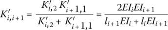
According to the finite segment model, the torsional springs ![]() and
and ![]() are introduced for two rigid segments of the series. The torsional stiffness coefficient between two rigid segments is
are introduced for two rigid segments of the series. The torsional stiffness coefficient between two rigid segments is
The moment and rotation angle between the two rigid segments can be obtained from
where ![]() is the elastic moment between two rigid segments, and
is the elastic moment between two rigid segments, and ![]() and θi are the orientation angles of the (
and θi are the orientation angles of the (![]() )th rigid segment and the ith rigid segment, respectively.
)th rigid segment and the ith rigid segment, respectively.
Similarly, considering the torsion and compression deformation of the beam, we obtain
where ![]() is the elastic force between rigid segments, namely the internal force between rigid segments, and
is the elastic force between rigid segments, namely the internal force between rigid segments, and ![]() and xi are the position coordinates of the hinge point of the (
and xi are the position coordinates of the hinge point of the (![]() )th rigid segment and the ith rigid segment, respectively.
)th rigid segment and the ith rigid segment, respectively.
Similar to the above derivation, the elastic coefficient of the linear spring between two rigid segments is
where EA is the extensional rigidity coefficient.

Figure 9.20 Plane‐motion cantilever mounted on a rotary base.
Figure 9.21 Time history of the driving moment.

Figure 9.22 Time history of the transverse deformation of a tip end.
Figure 9.23 Time history of the longitudinal deformation of a tip end.
Figure 9.24 Time history of rotation angular velocity.
Figure 9.25 Relation between computational time and number of segments.
9.5 Transfer Matrix Method for Controlled Multibody Systems I
In reference [251], the control signal is regarded as the state variable of a state vector. The TMM is extended to control of a chain multibody system for modal analysis of the controlled multi‐link mechanical arms. The computational method for the dynamics of a real‐time controlled system, whose control force is related to the current system state, is introduced in this section. By taking the control characteristic parameters of the system as special mechanical parameters and re‐deriving the transfer matrices of controlled elements, there is no need to add the state variables corresponding to the control signal. The dynamics of controlled multibody systems can be studied by the MSTMM [77]. For a time‐delay controlled multibody system, the control force can be denoted by the previous system state and regarded as an external force, and only the control forces in the terms of the external force column matrix of the MSTMM need to be considered. The dynamics of the controlled system can be solved using the same methods of the MSDTTMM.
9.5.1 Transfer Matrix Method for Linear Real‐time Controlled Multibody Systems
9.5.1.1 Dynamic Model of Linear Controlled Multibody Systems
For the linear controlled multibody system shown in Figure 9.26, Kj and ![]() denote the elastic coefficient of the spring and viscous damping coefficient of element j, respectively. The simple harmonic external force with frequency Ω acting on lumped mass mj
denote the elastic coefficient of the spring and viscous damping coefficient of element j, respectively. The simple harmonic external force with frequency Ω acting on lumped mass mj![]() is
is
Figure 9.26 Dynamic model of a linear controlled multibody system.
The sensor of the controlled system is fixed on lumped mass mk and the real‐time control force acting on the lumped mass mp produced by the controller is
9.5.1.2 Transfer Equation and Extended Transfer Matrix of Elements
According to the method given in Section 2.7, when the system is in steady‐state motion, the motion of every lumped mass may be indicated by
where ![]() is the complex amplitude of the steady‐state forced vibration.
is the complex amplitude of the steady‐state forced vibration.
The complex amplitude of the simple‐harmonic external force can be written as
Substituting Equation (9.14) into Equation (9.13), the control force of the controlled element is
The complex amplitude of the control force is
According to the geometrical relationship and the force balance condition of the two ends of the controlled lumped mass p, we can obtain
Substituting Equation (9.17) into Equation (9.18), these equations can be written in the following matrix form
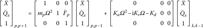
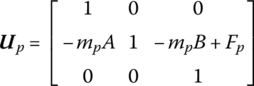
Thus, the transfer equation of the real‐time controlled element p is
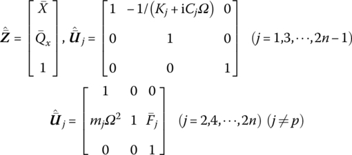
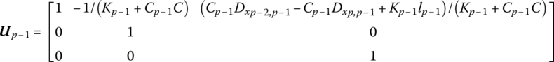
The extended transfer equation of other elements without control is
where
9.5.1.3 Overall Transfer Equation and Overall Transfer Matrix
From Equations (9.20) and (9.21), we obtain
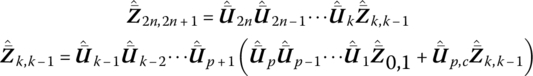
The second formula of Equation (9.23) yields
Substituting Equation (9.24) into the first formula of Equation (9.23), the overall transfer equation is obtained
where the overall transfer matrix is
9.5.1.4 Solving the Steady‐state Motion of the System
The boundary conditions of the system are
Substituting Equation (9.27) into Equation (9.25) yields
Solving Equation (9.28), the unknown state variables in the state vector of the system boundary can be obtained
By using Equation (9.21) in sequence and Equation (9.20), the state vectors at any point of the system can be determined. Therefore, the complex amplitude ![]() of each lumped mass can be obtained. From Equation (9.14), the steady‐state motion can be obtained
of each lumped mass can be obtained. From Equation (9.14), the steady‐state motion can be obtained
Figure 9.27 A linear multibody vibration system with a controlled loop.
Figure 9.28 The computational results of system dynamics. (a) Time history of the location coordinate of lumped mass 2. (b) Time history of the location coordinate of lumped mass 4. (c) Time history of the location coordinate of lumped mass 6.
Figure 9.29 Frequency response for a linear controlled multibody system with a controlled loop. (a) Frequency response for Ka = 0. (b) Frequency response for Ka = 5.0.
Figure 9.30 Linear controlled multibody system with a controlled loop.
Figure 9.31 Time history of the dynamics of a system: (a) time history of the displacement of lumped mass 2, (b) time history of the displacement of lumped mass 4 and (c) time history of the displacement of lumped mass 6.
Figure 9.32 Model of a branch multibody system.
Figure 9.33 Time history of the angular velocity of element 5 around the x axis.
Figure 9.34 Time history of the angular velocity of element 5 around the y axis.
Figure 9.35 Time history of the angular velocity of element 5 around the z axis.
9.5.2 Transfer Matrix Method for Linear Delay Controlled Multibody Systems
A linear controlled multibody system is shown in Figure 9.26. If the system has a time delay τ and steady‐state motion, the motion of a lumped mass can be denoted by
where ![]() is the complex amplitude of the steady‐state forced vibration.
is the complex amplitude of the steady‐state forced vibration.
The control force is
Equation (9.41) can be written as
The complex amplitude of the control force is
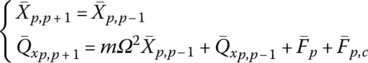
Taking the known control force Fp,c of the current time into the transfer matrix of the controlled element, the transfer equation of the controlled element is

namely
The overall transfer matrix is
According to the boundary conditions of the system and the transfer relation, the complex amplitude of each lumped mass ![]() can be obtained. The steady‐state motion can be obtained from Equation (9.40):
can be obtained. The steady‐state motion can be obtained from Equation (9.40):
Figure 9.36 The time history of the motion of a controlled system with time delay: (a) time history of the displacement of lumped mass 2, (b) time history of the displacement of lumped mass 4 and (c) time history of the displacement of lumped mass 6.
9.6 Transfer Matrix Method for Controlled Multibody Systems II
In this section, using the system in Figure 9.37 as an example, the discrete time transfer matrix method (DTTMM) for controlled multibody systems [78], developed by the authors, is introduced.
Figure 9.37 Controlled multibody system.
9.6.1 Discrete Time Transfer Matrix Method of Real‐time Controlled Multibody Systems
The DTTMM for multi‐rigid‐body systems was introduced in Chapter 7. The transfer equations of a lumped mass and a spring with longitudinal motion (see Figure 9.38) are obtained as follows
Figure 9.38 The subsystem composed of a spring and a lumped mass.
The state vector is
The transfer matrix of the spring is
The transfer matrix of the lumped mass is
Linearizing the real‐time control force as shown in Equation (9.13), this can be written as
From the geometry relation and the force equilibrium condition of element p, we have
Substituting Equation (9.53) into Equation (9.54), the transfer equation of the controlled element p is
where
From the system structure we can obtain

From the second formula of Equation (9.57), we have
Substituting Equation (9.58) into Equation (9.57), the overall transfer equation is
The overall transfer matrix is
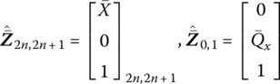
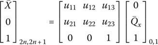
Substituting the boundary conditions ![]() and
and ![]() into Equation (9.53) yields
into Equation (9.53) yields

Hence
The state vector of each element in the system at any time can be solved using Equations (9.48) and (9.49) repeatedly, and Equation (9.55).

Figure 9.39 Time history of system motion with or without control: (a) time history of the displacement of lumped mass 2, (b) time history of the displacement of lumped mass 4 and (c) time history of the displacement of lumped mass 6.
Figure 9.40 Time history of system motion: (a) time history of the displacement of lumped mass 2, (b) time history of the displacement of lumped mass 4 and (c) time history of the displacement of lumped mass 6.
Figure 9.41 Time history of system motion: (a) time history of the displacement of lumped mass 2, (b) time history of the displacement of lumped mass 4 and (c) time history of the displacement of lumped mass 6.

Figure 9.42 Model of a controlled planar flexible manipulator.
The following assumptions are made for system modeling:
- The thickness of the bond for each PZT actuator and the flexible arm is too thin to have a deep effect on dynamics of the system, thus is neglected.
- The PZT actuators are rigidly bonded to the flexible arm.
- The thickness of each PZT actuator is transparent, and their effects on the mass distribution and stiffness distribution of system are neglected. The flexible arm is considered to be a uniform cross‐section Euler–Bernoulli beam.
- The voltage of each PZT actuator is uniformly distributed. The polarization direction of each PZT is the same as the transverse vibration direction of the corresponding flexible arm. The trajectory tracking and active vibration control of the flexible arm are studied by combining the proportional‐differential (PD) feedback control and the modal velocity feedback control.
The control moments acting on the hub rigid body and the driving voltage applied to the ith segmented PZT are, respectively
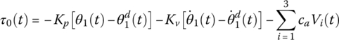
where ![]() and
and ![]() are the desired angle and angular velocity of hub rigid body 1, respectively, θ1 and
are the desired angle and angular velocity of hub rigid body 1, respectively, θ1 and ![]() are the actual angle and angular velocity, respectively, Kp and Kv are the proportion gain and velocity gain, respectively, τ0(t) is the control moment for drive motor, Kai is the gain coefficient of the ith segmented PZT actuator, Vi is the driving voltage applied to the ith segmented PZT actuator, u is the transverse deformation of the flexible arm, Yk(x2) is the kth
are the actual angle and angular velocity, respectively, Kp and Kv are the proportion gain and velocity gain, respectively, τ0(t) is the control moment for drive motor, Kai is the gain coefficient of the ith segmented PZT actuator, Vi is the driving voltage applied to the ith segmented PZT actuator, u is the transverse deformation of the flexible arm, Yk(x2) is the kth ![]() model function of the flexible arm, and
model function of the flexible arm, and ![]() .
. ![]() is the position coordinate of each PZT on the corresponding flexible arm in the body‐fixed reference coordinate system.
is the position coordinate of each PZT on the corresponding flexible arm in the body‐fixed reference coordinate system.
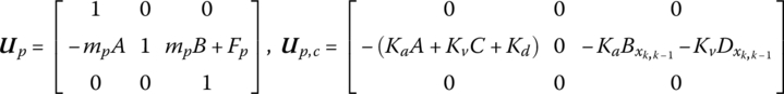
Considering only the control moment on the rigid body related to its feedback state, the transfer matrix of the controlled rigid body vibrating in a plane is
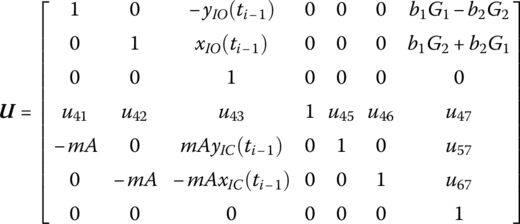
where
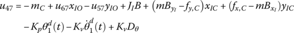
u41, u42, u45, u46, u57 and u67 are the same as in Equation (7.101).
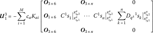
Using Equations (9.66) to (9.68), and considering the control moment of the PZT actuators, the transfer matrix of the controlled piezoelectric beam vibrating in a plane is
where
b and tb are the width and thickness of the flexible arm, respectively. ta is the thickness of the segmented PZT actuator.
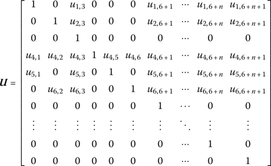
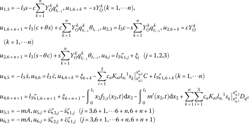
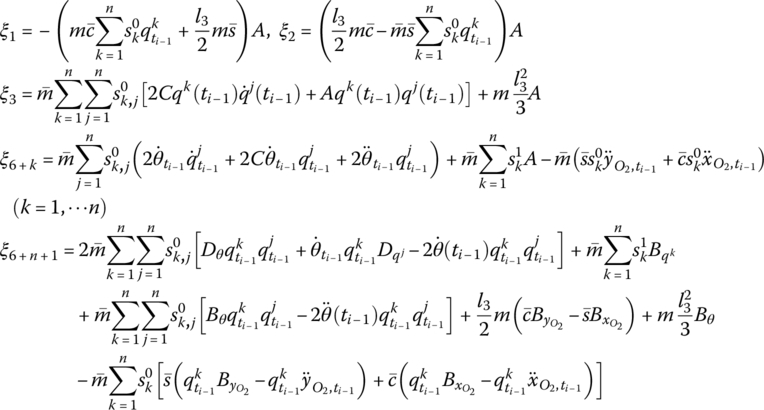
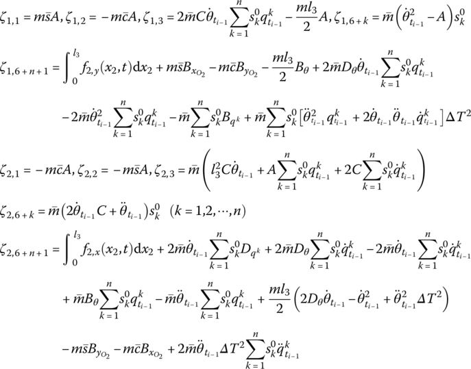
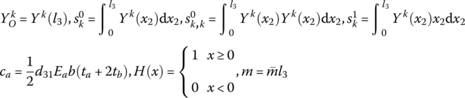
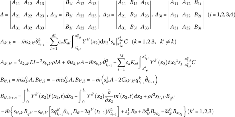
For the fixed hinge whose inboard body is a rigid body and whose outboard body is a piezoelectric beam with large planar motion the position coordinates, orientation angles, internal moments and internal forces of the rigid body’s input and output are equal. The transfer relation between the generalized coordinates describing the deformation of the outboard flexible body and the input end of the fixed hinge only needs to be determined. The dynamics equation of the transverse vibration of the beam is given by Equation (8.91) and the highest order of the mode shapes is chosen to be 3. The distributed moments of the PZT actuators and the control equation of the PZT actuators should be taken into consideration when we deduce the transfer equation of the beam. The state vectors of the fixed hinge whose input end is a rigid body and output end is a piezoelectric beam with large planar motion are defined as
The transfer equation is
The transfer matrix is
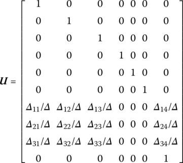
where
For compound control by the PD controller and modal velocity feedback control based on PZT actuators, the transfer matrix ![]() of the control element is
of the control element is
where ![]() is the feedback parameter matrix related to the feedback parameter from feedback beam 3 to hub 1.
is the feedback parameter matrix related to the feedback parameter from feedback beam 3 to hub 1.
For the modal velocity feedback control, we have
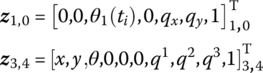
According to the DTTMM for controlled multibody systems, the state vectors of the system are
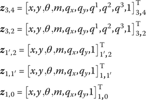
The boundary conditions are
The overall transfer equation is
where ![]() ,
, ![]() ,
, ![]() and
and ![]() are determined by Equations (9.67), (9.70), (9.66) and (9.71), respectively.
are determined by Equations (9.67), (9.70), (9.66) and (9.71), respectively.
The dynamics of the controlled flexible manipulator system calculated by the DTTMM for controlled multibody systems are shown in Figure 9.43. The time history of the expected orientation angle of the body‐fixed reference system of flexible arm 3 is shown in Figure 9.43a. The time history of the transverse deformation at the tip of arm 3 with and without PZT active control is shown in Figure 9.43b. The driving voltage applied to segmented PZT 1 is shown in Figure 9.43c. The simulation results show that the orientation angle of the flexible manipulator and expected track have good agreement. The transverse deformation at the tip of the arm decreases quickly. This validates the DTTMM for controlled multibody systems for the solution of the trajectory tracking of the flexible manipulator and active control of vibration.

Figure 9.43 Dynamics of a controlled flexible manipulator system: (a) time history of the orientation angle of a flexible arm, (b) time history of the transverse deformation at the tip of the arm and (c) time history of the driven voltage applied to segmented PZT 1.
Figure 9.44 Multibody system composing of a rigid body and an elastic hinge moving in space.

Figure 9.45 Time history of the angle of a rigid body around the z axis.
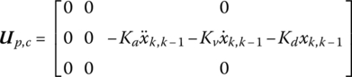
9.6.2 Discrete Time Transfer Matrix Method for Controlled Multibody Systems with Time Delay
For a controlled system with time delay, the control force in Equation (9.13) with time delay can be described as the function of the former motion parameters ![]() ,
, ![]() and
and ![]() as follows
as follows
where τ is the time delay.
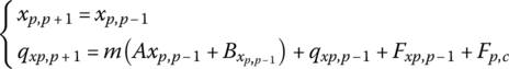
For the controlled system with time delay, substituting Equation (9.81) into Equation (9.54) and replacing u23 of the control transfer matrix by the known control force Fp,c in current time yields
For the controlled system with time delay, the current control force is the function of the former force and can be regarded as an external force. The elements of ![]() are all known functions of the previous time step, and Equation (9.60) can be written as
are all known functions of the previous time step, and Equation (9.60) can be written as
Applying the boundary conditions of the system and using Equations (9.48) and (9.49) repeatedly, the state vectors of each element at any time can be obtained.

Figure 9.46 Time history of system motion: (a) time history of the displacement of lumped mass 2, (b) time history of the displacement of lumped mass 4 and (c) time history of the displacement of lumped mass 6.