
2
Transfer Matrix Method for Linear Multibody Systems
2.1 Introduction
Strictly speaking, various engineering mechanism systems, such as machine tools, weaponry, carrier rockets, airplanes and vehicles as well as electromechanical systems with controllers, are nonlinear and time‐variant multi‐flexible‐body systems (MFSs). However, the accuracy could also be achieved in many situations even if a linear model of a multi‐rigid‐flexible‐body system is used for an engineering project as then it becomes easy to solve actual engineering problems. The dynamics model of linear MRFSs has therefore become one of the most popular, most important and most practical physical models in engineering fields such as weaponry, shipping, aeronautics, astronautics, communications, general machineries etc. The problems of linear multibody system dynamics (MSD) that are of interest to scientists and engineers include eigenvalue problems, vibration characteristics, steady‐state responses, the orthogonality of eigenvectors and the dynamic responses of linear multibody systems (MSs).
Vibration characteristics are one of the most important dynamics characteristics of mechanical systems. It is hard to obtain justifiable dynamic performance of the mechanical system if the vibration characteristics cannot be solved or pre‐estimated exactly when designing it. It is therefore very important to express exactly the vibration characteristics of MRFSs. For example, it has been shown by theory and experiment that the dynamic performance and firing precision of a multiple launch rocket system (MLRS) are influenced greatly by its vibration characteristics, firing frequency and firing orders. This is because different vibration characteristics of the MLRS induced by different firing orders lead to different initial disturbances of the rockets and different firing precision of the MLRS. To appraise the dynamics characteristics of a mechanical system scientifically, it is necessary to compute the vibration characteristics of the system exactly, therefore the exact expression of the vibration characteristics of the MRFS is an important component of MSD. If a quantitative relationship between the population parameters of the structure and the vibration characteristics can be developed for a weapons system, the vibration characteristics can be modified according to our prediction by changing the population parameters, and this offers a good base for the design of weapons with high firing precision. Evaluating the vibration characteristics of a MRFS exactly, including eigenfrequency, eigenvector and damping ratio, is the precondition to solve exactly the dynamic response of the MRFS under arbitrary excitation by using the modal analysis method. At present, the approaches used in researching the vibration characteristics of mechanical systems include the finite element method (FEM), the modal analysis method and the modal synthesis method. We have to deal with problems such as high‐order matrices, huge computational scale and computational ill‐condition problems when computing the vibration characteristics of a complex MRFS by using ordinary mechanics methods. It is an important long‐term aim in this field to reduce greatly the computational scale and avoid computational ill‐condition problems. The transfer matrix method for linear multibody systems has been developed by the authors and their co‐workers, thus the problems of huge computational scale and computational ill‐condition are avoided when the vibration characteristics are evaluated.
The basic idea of using the transfer matrix method for multibody system (MSTMM) to study MSD is as follows. A complicated MS can be broken up into elements containing bodies (rigid bodies, flexible bodies, lumped masses, etc.) and hinges (joints, ball‐and‐sockets, pins, springs, rotary springs, dampers and rotary dampers, etc.) with simple dynamics properties that can be readily expressed in matrix form. These matrices of elements are considered as the building blocks that provide the dynamics properties of the entire system when they are assembled according to the topology structure of the system, and are therefore called transfer matrices. The matrix formulation of any topology structure of the system is superbly adapted for consumption by computers. Furthermore the concise matrix notation brings to light basic properties of MSs formerly obscured in a mass of algebraic baroque. In particular, in the MSTMM the positions of bodies and hinges are considered equivalent in transfer matrices, and the order of the system matrix is independent of the number of degrees of freedom (DOF) of the system and dependent only on the order of the dynamics equations of the elements, which is totally different from ordinary MSD and results in a very low order of system matrix and very high computational speed. It is therefore not difficult to compute huge MSD with high DOF. A common type of MS occurring in engineering practice consists of a number of elements linked together end to end in the form of a chain, such as beams, turbine‐generator shafts, crankshafts, etc. The MSTMM is ideally suitable for such systems and the overall transfer matrix of the system can be obtained automatically by successive multiplications of matrices of elements to assemble the element. In the MSTMM, the overall transfer matrix of the system can be deduced automatically by using the transfer matrices of each element. The characteristic equation can be obtained from the overall transfer equation by using the boundary conditions of the system, from which the vibration characteristics can be computed.
In this chapter, the basic principles of the MSTMM developed by the authors, the eigenvalue problem [4, 41, 43–46] and steady‐state response of undamped systems and damped systems, including discrete and continuous MSs, and hybrid systems coupling discrete and continuous MSs composed of rigid bodies, lumped masses, beams, rods, shafts and so forth, are introduced. The dynamics problems of the flexible plate will be introduced in Chapter 4.
2.2 State Vector, Transfer Equation and Transfer Matrix
2.2.1 State Vector
The state vector at a point i of an MS is defined as a column matrix denoting the mechanics state of the point. The state variables of the state vector include the displacements of the point (including angular displacements) and the internal forces (including internal torques). Based on the sign conventions used in this book, ![]() denotes the state vector under physics coordinates and
denotes the state vector under physics coordinates and ![]() denotes the state vector under modal coordinates. The state vectors of different points are distinguished from each other by using different subscripts. For a nonboundary end, the first and second subscripts i and j (
denotes the state vector under modal coordinates. The state vectors of different points are distinguished from each other by using different subscripts. For a nonboundary end, the first and second subscripts i and j (![]() ) in a state vector
) in a state vector ![]() of the end denote the sequence numbers of the adjacent body element and hinge element, respectively. For a boundary end, the second subscript j = 0 in the state vector
of the end denote the sequence numbers of the adjacent body element and hinge element, respectively. For a boundary end, the second subscript j = 0 in the state vector ![]() , that is, the second subscript 0 means boundary end and the first subscript i in the state vector
, that is, the second subscript 0 means boundary end and the first subscript i in the state vector ![]() of the boundary end stands for the sequence number of the element involved.
of the boundary end stands for the sequence number of the element involved.
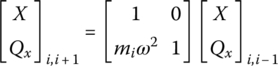
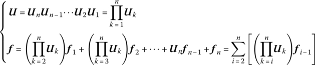
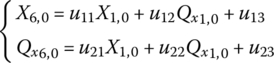
A chain system composed of three springs and three lumped masses with longitudinal vibration is shown in Figure 2.1. Consider the elements 1 and 6 as the root and tip of the system, respectively. According to the sign conventions used in this book, the transfer direction is from the tip to the root of the system, elements are numbered from 1 to 6 in sequence and the two boundary ends are numbered 0. The state vector at the connection point Pi,j is defined as
where xi,j and qxi,j are the displacement and internal forces of point Pi,j in the inertia coordinate system, respectively, subscripts i and j are the sequence numbers of the adjacent body element and hinge element, respectively, and superscript T means transposition. In other words, the state vector consists of displacement and corresponding internal force for a longitudinal vibration system.
Figure 2.1 Spring‐mass chain system.
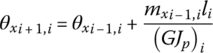
A torsion vibration system composed of an elastic massless shaft and disks concentrated at different points along its length is shown in Figure 2.2. Analogous to the longitudinal vibration system, the state vector is defined as
where θxi,j and mxi,j are the angular displacement and corresponding internal torque of point Pi,j in the inertia coordinate system, respectively. The state vector is composed of angular displacement and corresponding internal torque for the torsion vibration system.

Figure 2.2 Torsion vibration system of shaft disks.
A step beam system transversely vibrating in a plane is shown in Figure 2.3, and the state vector of the connection point Pi,j is defined as
where yi,j and θzi,j are the displacement and the angular displacement of point Pi,j in the y axis and about the z axis in the inertia coordinate system, respectively, and mzi,j and qyi,j are the corresponding internal torque and internal shear force of point Pi,j in the same inertia coordinate system, respectively, as shown in Figure 2.4.
Figure 2.3 Transverse vibration of a step beam system.

Figure 2.4 Transverse vibration of an elastic beam.
The state vector of an arbitrary point ![]() of the beam is defined as
of the beam is defined as
where li is the length of the ith beam element.
Notice the order of the state variables in the state vectors: the displacements are placed in the upper half of the column and the forces in the lower, in such a way that the forces and the corresponding displacements (i.e., y and qy, θz and mz) are in positions that are mirror images of each other about the center of the column. This arrangement has advantages that will be appreciated later.
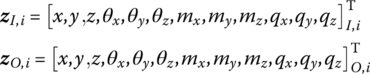
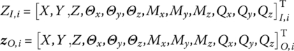
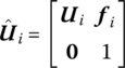
A spatial small vibration rigid body numbered i with one input end and one output end is shown in Figure 2.5, and the state vectors at the input and output ends are defined as
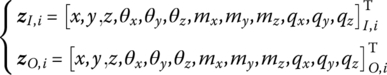
Figure 2.5 Rigid body with one input end and one output end.
The general principles used to define state vectors are as follows:
- The geometric position and mechanics state of each connection point of the system can be described completely.
- The number of state variables involved is as less as possible.
- It is convenient to build up the transfer equations.
For instance, a planar motion rigid body numbered i with two input ends and one output end is shown in Figure 2.6. The two input ends are connected with hinges ![]() and
and ![]() , respectively, and the output end is connected with hinge
, respectively, and the output end is connected with hinge ![]() . The state vectors of each connection point are defined as
. The state vectors of each connection point are defined as
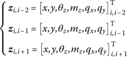
Figure 2.6 Planar motion rigid body with two input ends and one output end.
There are only three independent variables in the six displacement variants of the state vectors at the two input ends. Therefore, the state vector of the input end of the rigid body is defined as
or
where
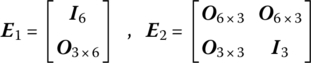
Nine independent variables in ![]() are used to describe completely the geometric and mechanics state of the input ends of the rigid body, including total state variables at the first input end
are used to describe completely the geometric and mechanics state of the input ends of the rigid body, including total state variables at the first input end ![]() and three forces and torques in the state variables of the second input end
and three forces and torques in the state variables of the second input end ![]() . None is dispensable.
. None is dispensable.
2.2.2 State Vector under Modal Coordinates
The response of undamped free vibration of MSs can be obtained by superposition of principal modals. The state vector of the system corresponding to eigenfrequency ωk under the kth modal can be expressed as
where i is the imaginary unit and ![]() is the state vector under the kth modal coordinates, whose variables are displacements and internal forces corresponding to eigenfrequency ωk.
is the state vector under the kth modal coordinates, whose variables are displacements and internal forces corresponding to eigenfrequency ωk.
According to the sign conventions used in this book, ![]() should be written as
should be written as ![]() . For conciseness, the superscript k of
. For conciseness, the superscript k of ![]() will be omitted and the term is abbreviated as
will be omitted and the term is abbreviated as ![]() when the modal orders are not emphasized. The detailed forms of the state vectors under modal and physics coordinates are shown in Table 2.1.
when the modal orders are not emphasized. The detailed forms of the state vectors under modal and physics coordinates are shown in Table 2.1.
Table 2.1 State vectors under modal coordinates and corresponding physics coordinates
| Research objects | State vectors | |
| Spring‐mass system | Physics coordinates |
|
| Modal coordinates |
|
|
| Torsion vibration system | Physics coordinates |
|
| Modal coordinates |
|
|
| Transverse vibration beam | Physics coordinates |
|
| Modal coordinates |
|
|
| Rigid body with one input end and one output end | Physics coordinates |
 |
| Modal coordinates |
 |
|
2.2.3 Transfer Equation and Transfer Matrix
To introduce the basic principles of MSTMM, transfer equations and transfer matrices of some basic mechanics elements are introduced here. Various transfer matrices of other elements involved in general MSs and their derivation methods are introduced in Chapter 10 and subsequent chapters.
2.2.3.1 Transfer Matrix of a Longitudinal Vibration Spring
The transfer equation and the transfer matrix of a longitudinal spring that is used in the chain spring‐mass system shown in Figure 2.1 are introduced. The free‐body diagram of the massless spring, as well as the positive directions of the displacements of its two ends and the forces acting on these two ends, are shown in Figure 2.7. We assume that the dynamic system is undergoing simple harmonic vibration and the eigenfrequency is denoted by ω. The stiffness of the spring is Ki and the state vectors of the input and output ends are ![]() and
and ![]() , respectively. From the equilibrium of forces acting on the spring and the stiffness property of the spring we obtain
, respectively. From the equilibrium of forces acting on the spring and the stiffness property of the spring we obtain
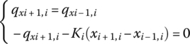
Figure 2.7 Free‐body diagram of a spring.
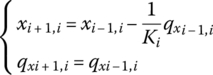
Equation (2.8) can be rewritten in the form
For simple harmonic vibration we have
Substituting Equation (2.10) into Equation (2.9) results in the corresponding equations in the modal coordinate, notated in a matrix form as
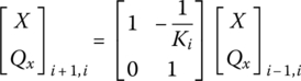
or
where
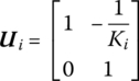
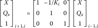
Equation (2.12) describes the relation of state vectors between the two ends of the spring. It means that the state vector of the output end ![]() of the element numbered i can be expressed using the state vector of the input end
of the element numbered i can be expressed using the state vector of the input end ![]() by using matrix
by using matrix ![]() . Therefore Equation (2.11) or Equation (2.12) is called the transfer equation of the spring. The bold italic capital
. Therefore Equation (2.11) or Equation (2.12) is called the transfer equation of the spring. The bold italic capital ![]() is the transfer matrix of the spring i.
is the transfer matrix of the spring i.
2.2.3.2 Transfer Matrix of Longitudinal Vibration Lumped Mass
The free‐body diagram of lumped mass mi in the longitudinal vibration system of Figure 2.1 is shown in Figure 2.8. The displacements at the left and right ends are equal, that is
Figure 2.8 Free‐body diagram of a lumped mass.
According to Newton’s second law, we obtain
Combining Equations (2.14) and (2.15) yields
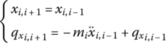
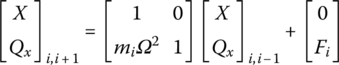
For the lumped mass mi with simple harmonic vibration, substituting Equation (2.10) in Equation (2.16) and compacting the results in a matrix form, we have
that is,
Equation (2.18) is the transfer equation of the longitudinal vibration lumped mass, where
is the transfer matrix of the lumped mass.
2.2.3.3 Transfer Matrix of a Torsion Vibration Massless Shaft
The free‐body diagram of the massless shafts with uniform cross‐section in a torsion vibration system of Figure 2.2 is shown in Figure 2.9. From the equilibrium of the internal torsion moments of its two ends, we have
Figure 2.9 Free‐body diagram of a shaft.
From the mechanics of materials
where G and GJp are the shear modulus of material and the torsion stiffness of the shaft, respectively.
Considering Equation (2.10), notate Equations (2.19) and (2.20) using the matrix, and then the transfer equation of the torsion vibration massless shaft can be obtained:
where
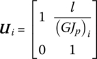
is the transfer matrix of the torsion vibration massless shaft.
2.2.3.4 Transfer Matrix of a Disk
The free‐body diagram of the rigid disks in the torsion vibration system of Figure 2.2, whose rotational inertia is Ji, is shown in Figure 2.10. The twist angles of its two ends are equal, that is,
Figure 2.10 Free‐body diagram of a disk.
The rotation equation is
Considering Equation (2.10) and rewriting Equations (2.23) and (2.24) in matrix form, the transfer equation can be obtained:
where
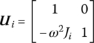
is the transfer matrix of the torsion vibration rigid disk.
2.2.3.5 Transfer Matrix of a Planar Transverse Vibration Massless Elastic Beam
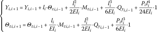
The free‐body diagram of a planar transverse vibration massless elastic beam is shown in Figure 2.11. Its length and bending stiffness are li and EIi, respectively, and its displacements and internal forces of its two ends are given based on the sign conventions. From the equilibrium condition of forces and moments, we obtain
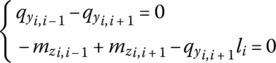

Figure 2.11 Free‐body diagram of a transverse vibration elastic beam.
According to the elementary theory of a beam, in the body‐fixed coordinate system with origin the input end of the beam, the displacement and slope of the output end are
where EI and l are the flexural rigidity and length.
Applying the above equations and taking note of the displacement ![]() and slope
and slope ![]() of the input end
of the input end ![]() , the displacement and the slope of the output end in the inertial coordinate system can be written as
, the displacement and the slope of the output end in the inertial coordinate system can be written as

Combining Equations (2.26) and (2.29) yields
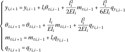
Furthermore, considering Equation (2.10) and rewriting Equation (2.30) in matrix form, the transfer equation can be deduced as
where
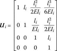
is the transfer matrix of the planar transverse vibration massless elastic beam.
It can be seen clearly that the transfer matrix describes the relation between the mechanics states of different space points at the same time. It transfers the state vectors from ![]() of point Pi,j to
of point Pi,j to ![]() of point Pm,n of the system. That is, it transfers the state from one place to another, so the transfer matrix is also called the state transform matrix. Generally speaking, for a simple‐harmonic vibration system with frequency ω, the transfer matrix is a function of ω, that is,
of point Pm,n of the system. That is, it transfers the state from one place to another, so the transfer matrix is also called the state transform matrix. Generally speaking, for a simple‐harmonic vibration system with frequency ω, the transfer matrix is a function of ω, that is, ![]() .
.
2.3 Overall Transfer Equation, Overall Transfer Matrix and Boundary Conditions
2.3.1 Overall Transfer Equation and Overall Transfer Matrix
A vibration system comprising n elements is used as an example, as shown in Figure 2.12, to show how to deduce the overall transfer equation and overall transfer matrix of the system. There are ![]() connection points and two boundary ends, and
connection points and two boundary ends, and ![]() are the boundary state vectors.
are the boundary state vectors.

Figure 2.12 An elastic beam with several lumped masses.
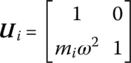
The transfer equations of the n elements are
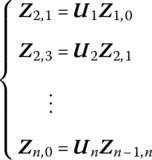
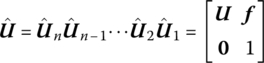
The overall transfer equation of the system is
where
is the overall transfer matrix of the system, which is obtained by successively multiplying each element’s transfer matrix of the system in sequence.
In the overall transfer equation, apart from the boundary state vectors no state vectors of other connection points are involved.
2.3.2 Boundary Conditions
The state vectors at the boundaries are composed of displacements and internal forces, and the number m of its components is always an even number. Generally, the components of state vectors at the boundaries are partly unknown. For homogeneous boundary conditions, half of the components are zeros and the others are unknown. Examples are as follows:
- In the transverse vibration system shown in Figure 2.13a, both ends of points P1,0 and P9,0 are free, and the internal forces and the internal moments are zero, whereas displacements are unknown. The boundary conditions are
- Point P1,0 is fixed and point P9,0 is free, as shown in Figure 2.13b. The boundary conditions are(2.36)

- If both points P1,0 and P9,0 are simply supported, as shown in Figure 2.13c, the boundary conditions are(2.37)

Figure 2.13 Examples of boundary conditions.
2.4 Characteristic Equation
For the transverse vibration system shown in Figure 2.12 the overall transfer Equation (2.33) of the system can be written as
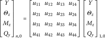
where the components ![]() of the transfer matrix are functions of the eigenfrequencies of the system.
of the transfer matrix are functions of the eigenfrequencies of the system.
Applying the boundary conditions, the following two homogeneous equation can be obtained
where ![]() consists of the two unknown components of state vector
consists of the two unknown components of state vector ![]() .
.
A nontrivial solution of the system is possible if and only if ![]() , so the value of the determinant of matrix
, so the value of the determinant of matrix ![]() is zero, that is
is zero, that is
where ![]() is a function of ω and Equation (2.40) is the characteristic equation of the system. For an undamped system, Equation (2.40) is usually known as the frequency equation and its roots are the eigenfrequencies of the system. For a damped system, the unknown components of the transfer matrix are complex numbers and the solutions of Equation (2.40)
is a function of ω and Equation (2.40) is the characteristic equation of the system. For an undamped system, Equation (2.40) is usually known as the frequency equation and its roots are the eigenfrequencies of the system. For a damped system, the unknown components of the transfer matrix are complex numbers and the solutions of Equation (2.40)
![]() are called eigenvalues. The real part
are called eigenvalues. The real part ![]() is related to the magnitude of damping, and the imaginary part λi is related to the eigenfrequency of the damped system. For the three kinds of boundary conditions mentioned above, the frequency equations of the undamped system are discussed as follows.
is related to the magnitude of damping, and the imaginary part λi is related to the eigenfrequency of the damped system. For the three kinds of boundary conditions mentioned above, the frequency equations of the undamped system are discussed as follows.
- Both ends of P1,0 and P9,0 are free boundaries, as shown in Figure 2.13a. Substituting boundary condition Equation (2.35) into Equation (2.38), we obtain(2.41)
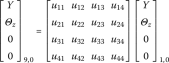
Picking out the third and fourth formulas of the homogeneous equations and rewriting them in form of Equation (2.39), we obtain
(2.42)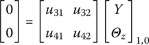
If there exist nontrivial solutions of the system, namely
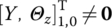 , then the frequency equation can be obtained:
 - Point P1,0 is fixed and point P9,0 is free, as shown in Figure 2.13b. The frequency equation is obtained using the proposed method:
- Both ends of P0,1 and P9,0 are simply supported, as shown in Figure 2.13c. The frequency equation is obtained using the proposed method:


Figure 2.14 A massless elastic simply supported beam with a lumped mass at the midpoint.
Figure 2.15 Free‐body diagram of a mass.
Figure 2.16 A 2 DOF spring‐mass system.
2.5 Computation for State Vector and Vibration Characteristics
The computation for the eigenfrequencies of a vibration system involves matrix multiplication. For a simple mass‐spring system, only simple multiplication of second‐order square matrices is involved. However, because of the high order of matrices for a complex system, the calculation by hand is very difficult and a computer has to be used. The computation of the eigenfrequencies of a system is usually done by combining the step‐by‐step scanning method and the dichotomy method, which is carried out by a computer. First, a series of tentative frequencies determined by the selected step should be chosen, such as ω, ![]() ,
, ![]() . The determinant value Δ of the characteristic equation (2.40) under each tentative frequency is then computed. If the Δ values corresponding to two adjacent tentative frequencies have opposite signs, there must be at least one frequency between them satisfying
. The determinant value Δ of the characteristic equation (2.40) under each tentative frequency is then computed. If the Δ values corresponding to two adjacent tentative frequencies have opposite signs, there must be at least one frequency between them satisfying ![]() . Thus, one of the regions of system eigenfrequencies is obtained. The eigenfrequencies can then be found using dichotomy in the regions. Setting ω as the horizontal axis and Δ as the vertical axis, we can obtain a point at this coordinate system for each tentative computation. Linking these points, the curve of ω ‐ Δ(ω) can be obtained, as shown in Figure 2.17. The intersection points of the curve and the axis of abscissa correspond to eigenfrequencies
. Thus, one of the regions of system eigenfrequencies is obtained. The eigenfrequencies can then be found using dichotomy in the regions. Setting ω as the horizontal axis and Δ as the vertical axis, we can obtain a point at this coordinate system for each tentative computation. Linking these points, the curve of ω ‐ Δ(ω) can be obtained, as shown in Figure 2.17. The intersection points of the curve and the axis of abscissa correspond to eigenfrequencies ![]() .
.
Figure 2.17 Plot of ω ‐ Δ(ω).
Figure 2.18 The ω ‐ Δ(ω) curves under the three kinds of boundary conditions: (a) free–free, (b) fixed–free and (c) both simply supported.
Table 2.2 Computation results of eigenfrequencies under the three boundary conditions (rad/s)
| Boundary conditions Order | Free–Free | Fixed–Free | Both simply supported |
| 1 | 0 | 0.146 | 0.343 |
| 2 | 0 | 1.080 | 1.593 |
| 3 | 1.789 | 3.144 | 3.754 |
| 4 | 4.000 | 5.731 | 5.274 |
Figure 2.19 The eigenvectors of the 2 DOF spring‐mass system.
Figure 2.20 The eigenvectors of a simply‐simply supported system: (a) first‐order eigenvector, (b) second‐order eigenvector, (c) third‐order eigenvector and (d) fourth‐order eigenvector.
Figure 2.21 The eigenvectors of the free–free beam system corresponding to  : (a) first‐order eigenvector and (b) second‐order eigenvector.
2.6 Vibration Characteristics of Multibody Systems
2.6.1 Vibration Characteristics of Discrete Systems
Figure 2.22 Chain discrete system.
Table 2.3 Computational results of eigenfrequencies
| Mode | 1 | 2 | 3 | 4 | 5 | 6 |
| Eigenfrequencies/(rad/s) | 10.98 | 31.62 | 48.45 | 59.43 | 64.24 | 196.47 |
| Mode | 7 | 8 | 9 | 10 | 11 | 12 |
| Eigenfrequencies/(rad/s) | 334.78 | 417.66 | 727.58 | 1606.10 | 2394.15 | 2916.31 |
Figure 2.23 Eigenvectors of the discrete system.
2.6.2 Vibration Characteristics of Continuous Systems
Figure 2.24 Elastic beam with uniform cross‐section.
Table 2.4 Computational results of eigenfrequencies
| Order | 1 | 2 | 3 | 4 | 5 | 6 | 7 | 8 |
| ωk (rad/s) | 51.40 | 322.1 | 901.9 | 1767.3 | 2921.5 | 4364.2 | 6095.4 | 8115.2 |
| λkl | 1.8751 | 4.6941 | 7.8548 | 10.9955 | 14.1372 | 17.2788 | 20.4204 | 23.5619 |
Figure 2.25 Eigenvectors of the continuous system.
Table 2.5 Computational results of eigenfrequencies
| Order | 1 | 2 | 3 | 4 | 5 | 6 | 7 | 8 |
| ωk (rad/s) | 51.40 | 321.9 | 900.7 | 1763.1 | 2910.4 | 4340.2 | 6049.5 | 8035.2 |
Figure 2.26 Eigenvectors of the Timoshenko beam.
Table 2.6 Vibration characteristics of a Euler–Bernoulli beam with uniform cross‐section
Table 2.7 Vibration characteristics of a straight rod with uniform cross‐section
| Boundary condition | Frequency equation | βkl | Function of eigenvector |
  |
|
 |
|
  |
|
 |
|
 |
|
 |
|
Note: ck is an arbitrary nonzero constant.
Table 2.8 Vibration characteristics of an elastic shaft with uniform cross‐section
| Boundary condition | Frequency equation | γkl | Function of eigenvector |
  |
|
 |
|
  |
|
 |
|
 |
|
 |
|
Note: ck is an arbitrary nonzero constant.
Figure 2.27 Transverse vibration of nonuniform beam.
Table 2.9 Computational results of eigenfrequencies for a nonuniform beam
| Order | Timoshenko beam | Euler–Bernoulli beam | |||||
| n = 100 | n = 10 | n = 100 | n = 10 | ||||
| ωk (rad/s) | ωk (rad/s) | Error (%) | ωk (rad/s) | Error (%) | ωk (rad/s) | Error (%) | |
| 1 | 155.3 | 150.6 | –3.03 | 155.4 | 0.06 | 150.6 | –3.03 |
| 2 | 443.8 | 367.1 | –17.28 | 444.1 | 0.07 | 367.3 | –17.24 |
| 3 | 873.7 | 621.4 | –28.88 | 874.6 | 0.10 | 621.8 | –28.83 |
| 4 | 1440.9 | 1120.3 | –22.25 | 1443.1 | 0.15 | 1121.8 | –22.15 |
| 5 | 2134.4 | 1873.3 | –12.23 | 2138.9 | 0.21 | 1877.6 | –12.03 |
| 6 | 2928.5 | 2831.6 | –3.31 | 2936.1 | 0.26 | 2840.2 | –3.02 |
| 7 | 3779.9 | 3682.2 | –2.58 | 3791.3 | 0.30 | 3692.4 | –2.31 |
| 8 | 4696.3 | 4728.8 | 0.69 | 4713.7 | 0.37 | 4754.5 | 1.24 |
2.6.3 Vibration Characteristics of a Hybrid System of Rigid and Flexible Bodies
Figure 2.28 A multi‐rigid‐flexible‐body system.
Table 2.10 Computational results of eigenfrequencies
| Order | 1 | 2 | 3 | 4 | 5 | 6 | 7 | 8 | 9 | 10 |
| ωk (rad/s) | 10.7 | 20.7 | 143.7 | 372.0 | 925.7 | 1783.3 | 2934.0 | 4374.8 | 6104.8 | 8123.8 |
Figure 2.29 Eigenvectors of the hybrid system of rigid and flexible Bodies.
Discussion
- If the system only includes element 1 and element 2, the eigenfrequencies should be
 and
and  . However, the first two eigenfrequencies are
  and
and  , respectively. The reason is that the mass of element 3 increases the total mass and the total moment of inertia of the system, which results in a decrease in the basic frequencies.
 - The computational results of the eigenfrequencies of a cantilever beam are shown in the second row of Table 2.11. Compared with Table 2.10, the eigenfrequencies of the higher modes are closer to those of the cantilever beam. Let the mass of rigid body 2 be
 . The computational results are shown in the third row of Table 2.11. Compared with the cantilever beam, the mass of rigid body 2 is much larger and the higher‐order eigenfrequencies can be substituted by the eigenfrequencies of the cantilever beam. The lower‐order eigenfrequencies of the system can be substituted by
  and
and  .
. - If
 in the system, the rigid body and beam can only vibrate vertically but cannot move horizontally. The eigenfrequencies are shown in Table 2.12. It is obvious that the eigenfrequencies are closer to that of the cantilever beam along with the increasing order of the mode.
Table 2.11 Eigenfrequencies comparison for ![]() and cantilever beam (rad/s)
and cantilever beam (rad/s)
| Order | 1 | 2 | 3 | 4 | 5 | 6 | 7 | 8 | 9 | 10 |
| Cantilever beam | − | − | 51.40 | 322.1 | 901.9 | 1767.3 | 2921.5 | 4364.2 | 6095.4 | 8115.2 |
| m2 =7800 kg | 0.3580 | 2.138 | 51.63 | 322.1 | 901.9 | 1767.3 | 2921.5 | 4364.2 | 6095.5 | 8115.3 |
Table 2.12 Computational results of eigenfrequencies when ![]() (rad/s)
(rad/s)
| Order | 1 | 2 | 3 | 4 | 5 | 6 | 7 | 8 | 9 |
|
|
10.78 | 52.96 | 325.1 | 904.8 | 1770.2 | 2924.4 | 4367.1 | 6098.4 | 8118.2 |

Figure 2.30 A torsional vibration system.
Table 2.13 Computational results of eigenfrequencies
| Order | 1 | 2 | 3 | 4 | 5 | 6 | 7 | 8 |
| ωk (rad/s) | 0 | 340.0 | 446.2 | 4192.9 | 5031.4 | 12576.7 | 15092.0 | 16777.1 |
Figure 2.31 Eigenvectors of the torsional vibration system.
Table 2.14 Computational results of eigenfrequencies without considering the mass of the shaft
| Order | 1 | 2 | 3 |
| ωk (rad/s) | 0 | 340.3 | 446.4 |
2.6.4 Procedure to Compute the Vibration Characteristics of a Multibody System
A general procedure to compute the vibration characteristics of MRFS is shown in Figure 2.32. The detailed procedures are as follows.
- Develop the dynamics model of the MRFS. Break up the whole MRFS into various elements. Define the state vectors of each element.
- The transfer matrices of each element are written according to the dynamics equations of each element, the transfer direction and the connection styles with other elements.
- According to the topology of the system, the overall transfer equation and the overall transfer matrix are deduced automatically. For chain systems, the overall transfer matrix can be obtained only by successively multiplying the transfer matrices of the elements. The unknown variables in the overall transfer equation are the state vectors at the boundary points of the system, and the elements of the overall transfer matrix are functions of the structural parameters and eigenfrequencies of the system.
- Construct the characteristic equation by substituting the boundary conditions into the overall transfer equation.
- The eigenfrequencies
 of the system are determined by solving the characteristic equation.
 - For each eigenfrequency ωk, the state vectors at the boundary points can be evaluated by solving the overall transfer equation. The state vectors and eigenvectors of each point in the system can be obtained by using the transfer equations of each element.
Figure 2.32 Procedure to compute the vibration characteristics of the MRFS.
2.7 Eigenvalues of Damped Vibration
2.7.1 Damping Model
2.7.1.1 Viscous Damping
A spring‐damper system is shown in Figure 2.33. The spring coefficient and the viscous damping coefficient are K and C, respectively, and the spring and damping force P(t) is expressed by
where x is the elongation (deformation) and ![]() is the motion speed.
is the motion speed.
Figure 2.33 Spring‐damper system.
When the system vibrates harmonically with ![]() , frequency Ω and amplitude A, the energy dissipated per cycle is
, frequency Ω and amplitude A, the energy dissipated per cycle is
Obviously, the energy dissipated per cycle is proportional to the exciting frequency Ω.
2.7.1.2 Structural Damping
The damping coefficient may vary with the exciting frequency Ω as
This kind of damping is called structural damping, where K is the spring coefficient and g is a constant between 0.005 and 0.015. The damping coefficient of an aircraft structure behaves in this way. It has been proved by Veubeke [233] that this kind of damping is nonexistent in physics. The relationship between force and displacement for this kind of damping is
The current damping force of the structure damping satisfying Equation (2.66) depends on the behavior of the displacement x in the past, present and future. Obviously, such a physical phenomenon does not exist. However, the concept of structural damping is acceptable if the frequency is confined to a certain range. When the spring‐damper system undergoes harmonic vibration,
According to Equations (2.64) and (2.66), we obtain
Then, the energy dissipated per cycle
is a constant independent of the frequency Ω.
2.7.1.3 Complex Impedance
Rewrite Equation (2.68) as
where Re represents the real part of the complex expression in the parentheses.
Substituting Equation (2.71) into Equation (2.64) yields
Analogous to a typical expression in the electric theory
is called the complex impedance of viscous damping. Similarly, the complex impedance for structure damping is
The concepts of complex shear modulus and complex Young’s modulus can be developed from Equation (2.74). If Poisson’s ratio is still a real number, we have
In Equations (2.74) and (2.76), G is the shear modulus, E is Young’s modulus and g = 0.005–0.010 for a welded structure.
2.7.2 Free Vibration of a Damped System
2.7.2.1 Damped Spring‐Mass System
The equation of free vibration for a damped spring‐mass system, as shown in Figure 2.34, is
Figure 2.34 Damped spring‐mass system.
Its solution has the form
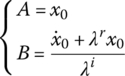
where the damping rate λr and the eigenfrequency λi are determined by Equation (2.77), and the constants A and B are determined by the initial conditions x0 and ![]() .
.
To determine λr and λi, Equation (2.78) is differentiated twice with respect to time, yielding
Substituting Equations (2.78), (2.79) and (2.80) into Equation (2.77) yields
Equation (2.81) holds true regardless of initial conditions, so

that is,
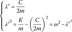
where ![]() is the eigenfrequency corresponding to the undamped system.
is the eigenfrequency corresponding to the undamped system.
Applying the initial conditions ![]() , the expressions for the constants A and B are
, the expressions for the constants A and B are
Only when λi is real, that is, when ![]() is positive, can the solution of Equation (2.77) exist, namely Equation (2.78) is valid. This means
is positive, can the solution of Equation (2.77) exist, namely Equation (2.78) is valid. This means 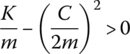 , namely
 ![]() . The system where the damping coefficient C is less than
. The system where the damping coefficient C is less than ![]() is called a light damped system. Most structures and mechanics systems may be regarded as light damped systems.
is called a light damped system. Most structures and mechanics systems may be regarded as light damped systems.
2.7.2.2 Complex Solution of Vibration
Let
where ![]() is a complex amplitude and λ is a complex eigenvalue with dimension 1/s.
is a complex amplitude and λ is a complex eigenvalue with dimension 1/s.
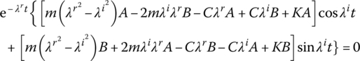
Substituting Equation (2.85) into Equation (2.77) yields the characteristic equation of the system
The complex eigenvalue can also be obtained:

Under the light damped situation (![]() ), this result coincides with Equation (2.83). Therefore, the solution of Equation (2.77) is
), this result coincides with Equation (2.83). Therefore, the solution of Equation (2.77) is
According to the Eulerian formula ![]() , the solution of Equation (2.77) can be written as
, the solution of Equation (2.77) can be written as
Because the right‐hand side of Equation (2.88) must be real, ![]() and
and ![]() must be conjugate complex numbers. Let
must be conjugate complex numbers. Let ![]() , then Equation (2.88) is reduced to Equation (2.78). Using the complex form, the expression of
, then Equation (2.88) is reduced to Equation (2.78). Using the complex form, the expression of ![]() can be easily obtained for common cases (not confined to light damped systems). The complex amplitude of a physics quantity under modal coordinates is denoted by a capital with a bar over it.
can be easily obtained for common cases (not confined to light damped systems). The complex amplitude of a physics quantity under modal coordinates is denoted by a capital with a bar over it.
2.7.3 Transfer Matrix Method for Free Vibration of Damped Multibody Systems
2.7.3.1 Complex Transfer Matrix
The forces of both ends of the spring‐damper system are equal, as shown in Figure 2.35, yielding
Figure 2.35 Free‐body diagram of a spring‐damper system.
The complex amplitudes of the forces are
The complex elastic force is
The complex internal forces at the two ends of the spring‐damper system are
hence
The complex transfer equation is
where
![]() is the complex transfer matrix of the spring‐damper.
is the complex transfer matrix of the spring‐damper.
For a lumped mass in a damped system, as shown in Figure 2.36, the relationship of displacements and forces between the two ends is
or
where
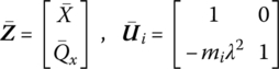
Figure 2.36 Free‐body diagram of a lumped mass in a damped system.
![]() is the complex transfer matrix of the lumped mass.
is the complex transfer matrix of the lumped mass.
2.7.3.2 Real and Imaginary Parts of the Complex Transfer Matrix
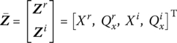
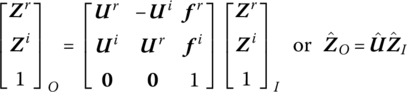
The complex state vectors and the complex transfer matrix can be split into real and imaginary parts and identified using the superscripts “r” and “i”, respectively. Then
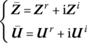
therefore
which can be rewritten in a matrix form as
Substituting ![]() into Equation (2.92b), the transfer matrix of the spring‐damper becomes
into Equation (2.92b), the transfer matrix of the spring‐damper becomes
Rewriting in the form of Equation (2.95) yields
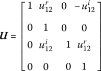
where
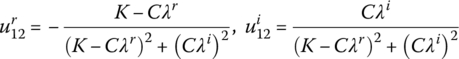
Similarly, the transfer matrix of the lumped mass is described as
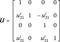
where ![]() and
and ![]() .
.
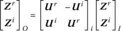
According to Equation (2.95) the state vector now consists of four elements:
When square matrices of the type in Equation (2.95) are multiplied, the result is a square matrix of the same type. This can be proved as follows:
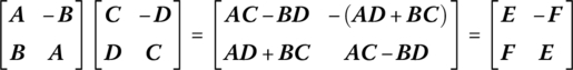
It is therefore necessary to carried out only half of the matrix multiplications.
2.7.3.3 Characteristic Equation
For the system shown in Figure 2.34, according to Equations (2.92) and (2.93), the overall transfer equation is obtained:

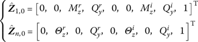
Substituting the boundary conditions ![]() into the overall transfer equation, the characteristic equation of the system is obtained:
into the overall transfer equation, the characteristic equation of the system is obtained:
Substituting ![]() into Equation (2.102) yields
into Equation (2.102) yields
therefore
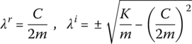
The complex eigenvalue of the damped system is obtained by solving the characteristic equation of the system.
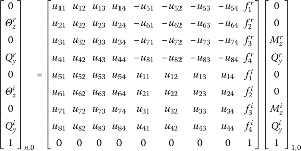
By repeating the above process with Equation (2.95), the overall transfer equation can be deduced as
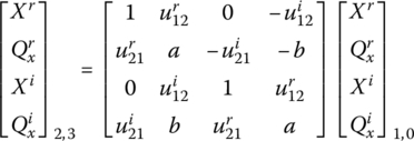
where
Substituting the boundary conditions ![]() into Equation (2.104) yields
into Equation (2.104) yields
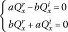
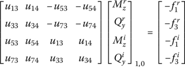
A nonzero solution of the system is possible if and only if
Both a and b are real numbers, therefore ![]() . By solving Equation (2.105), the complex eigenvalues of the system are obtained, which are identical to those in Equation (2.103).
. By solving Equation (2.105), the complex eigenvalues of the system are obtained, which are identical to those in Equation (2.103).
The characteristic equation of a complex multibody damped system can be obtained by using the two methods described. It can be seen from the above example that there are two unknown parameters λr and λi in the characteristic equation for a damped system, but only one unknown parameter of eigenfrequency in the characteristic equation for an undamped system. The numerical computation of eigenvalue problems for damped systems is therefore more difficult than for undamped systems. However, the TMM provides a powerful tool to compute the steady‐state response of the forced vibration of a damped system.
2.8 Steady‐state Response to Forced Vibration
After evaluating the eigenfrequencies and eigenvectors of a system using the TMM, the dynamic response of system including the transient response and steady‐state response to an arbitrary excitation can be solved. The system subjected to a simple‐harmonic excitation with frequency Ω will vibrate steadily with frequency Ω, and both the amplitude and phase of vibration depend on Ω. Based on this principle, the TMM can be applied to study the steady‐state forced vibration and the deformations and corresponding forces of static state of the system (![]() ).
).
2.8.1 Extended Transfer Matrix
In a system of spring‐mass steady‐state vibration with frequency Ω, as shown in Figure 2.39, the lumped masses are subjected to simple‐harmonic excitations F2 cos Ω t, F4 cos Ω t and F6 cos Ω t, respectively. Find the amplitude of the steady‐state responses of the system.
Figure 2.37 Forced vibration system of spring‐mass.
Figure 2.38 Free‐body diagram of a lumped mass in an undamped system.
Figure 2.39 A forced vibration of the 2 DOF spring‐mass system.
First, develop the extended transfer matrix of a lumped mass. The displacements of two ends of a lumped mass are equal, namely
As shown in Figure 2.38, from the equilibrium of the internal forces of the two ends, external force and inertia force, we get
Equations (2.108) and (2.109) can be expressed in matrix notation as
Equation (2.110) can be rewritten as an extended transfer equation

Notate the state vector ![]() and transfer matrix
and transfer matrix ![]() of forced vibration lumped mass as
of forced vibration lumped mass as
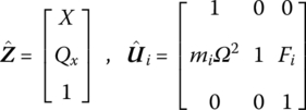
Then, Equation (2.111) is expressed as
where the state vector ![]() with components
with components ![]() ,
, ![]() and additional “1” is called the extended state vector of point
and additional “1” is called the extended state vector of point ![]() and the transfer matrix
and the transfer matrix ![]() is called the extended transfer matrix of lumped mass i.
is called the extended transfer matrix of lumped mass i.
Similar to Equation (2.111) for a lumped mass, the extended transfer equation of a spring i can be written as
2.8.2 Steady‐state Response to Forced Vibrations
Similar to the method for solving the eigenfrequencies and eigenvectors of a system, the overall transfer equation of a steady‐state vibration system can be obtained using the transfer equations of elements:
Notate the extended transfer matrix of element i as
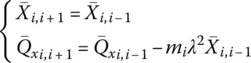
It can be proved that
If the sign of continued multiplication is used, which is defined as

then
where the form of ![]() is the same as the overall transfer matrix of the free vibrations system. However, the frequency in
is the same as the overall transfer matrix of the free vibrations system. However, the frequency in ![]() is not the eigenfrequencies ω but the excitation frequency Ω of the exciting forces, that is,
is not the eigenfrequencies ω but the excitation frequency Ω of the exciting forces, that is, ![]() .
.
Equation (2.114) can be expressed as
that is
When Ω is not equal to any of the eigenfrequencies ω, the unknown variables of Equation (2.119) can be easily solved with the boundary conditions. The boundary conditions of the system shown in Figure 2.37 are
Substituting this into Equation (2.119) gives
The state vectors, including the forces and displacements of an arbitrary point in the system, can be obtained by using the transfer matrices of the elements.

Figure 2.40 The frequency response of the 2‐DOFs spring‐mass system.
2.8.3 Forced Vibration of a Massless Beam
A transverse vibration massless beam subjected to a uniformly distributed harmonic load Pi cos Ω t is shown in Figure 2.41. From the equilibrium of forces and moments acting on the beam we get


Figure 2.41 A transverse forced vibration beam.
According to the Euler–Bernoulli beam theory,
Combining Equation (2.121) with Equation (2.122), the transfer equation of the beam can be described as
where
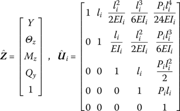
![]() is the extended transfer matrix of a vibration transverse massless beam subjected to a uniformly distributed harmonic load Pi cos Ω t and
is the extended transfer matrix of a vibration transverse massless beam subjected to a uniformly distributed harmonic load Pi cos Ω t and ![]() is the extended state vector of an arbitrary point of the beam.
is the extended state vector of an arbitrary point of the beam.
Figure 2.42 A beam under static load.
Figure 2.43 Computation results of deformation and distribution of moment and shear force: (a) displacement, (b) angular displacement, (c) bending moment and (d) shear force.
2.9 Steady‐state Response of Forced Damped Vibration
2.9.1 Response to Some Typical Excitations
2.9.1.1 Transient Response to an Impulse
The lumped mass of the damped system of Figure 2.34 is excited by an impulse G at time t0, and thereby it assumes the initial velocity
with ![]() , and the ensuing motion of mass m is given by Equations (2.78) and (2.84)
, and the ensuing motion of mass m is given by Equations (2.78) and (2.84)
2.9.1.2 Response to an Arbitrary Time‐variant Force
The lumped mass m of the damped system shown in Figure 2.34 is subjected to an arbitrary time‐variant force F(t) and an impulse F(t)dτ produces a velocity increment F(t)dτ/m at time τ. According to Equation (2.125), for ![]() the motion increment of mass m (
the motion increment of mass m (![]() ) due to the impulse is
) due to the impulse is
The resulting motion of m is obtained by integrating Equation (2.126) with respect to τ in time τ ≥ 0

If at time ![]() the initial conditions are nonzero, the motion of mass m is
the initial conditions are nonzero, the motion of mass m is

2.9.1.3 Steady‐state Forced Vibration of a Viscous Damping System
The lumped mass m of the viscous damped system shown in Figure 2.44 is subjected to a harmonic force with frequency, Ω, ![]() , which can also be represented as the real part of a complex function, that is
, which can also be represented as the real part of a complex function, that is
Figure 2.44 Viscous damped system.
The differential motion equation of lumped mass m is
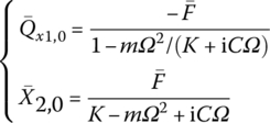
The particular solution of the differential Equation (2.129) which describes the steady‐state vibration of m is
where ![]() is the complex amplitude of the steady‐state forced vibration.
is the complex amplitude of the steady‐state forced vibration.
Substituting Equation (2.130) into Equation (2.129) gives
from which
The physics meaning of Equation (2.131) can be represented in the complex plane shown in Figure 2.45. If the displacement vector is ![]() , the spring force
, the spring force ![]() is parallel to
is parallel to ![]() . The effect of multiplication by i is to rotate the vector
. The effect of multiplication by i is to rotate the vector ![]() counterclockwise through 90° so that the direction of the damping force
counterclockwise through 90° so that the direction of the damping force ![]() is at 90° to
is at 90° to ![]() . The direction of inertia force
. The direction of inertia force ![]() is opposite to that of
is opposite to that of ![]() .
.
Figure 2.45 Force vectors in the complex plane.
From Figure 2.45, the magnitude ![]() and the phase‐lag angle α should satisfy
and the phase‐lag angle α should satisfy

therefore ![]() . (Note: a minus sign is positioned before α.) Substituting this into Equation (2.130) gives
. (Note: a minus sign is positioned before α.) Substituting this into Equation (2.130) gives
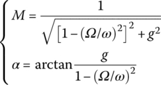
Introducing the eigenfrequency of undamped free vibration ![]() and dimensionless damping ratio
and dimensionless damping ratio ![]() , from Equation (2.134) the magnitude
, from Equation (2.134) the magnitude ![]() and the phase‐lag angle α can be written as
and the phase‐lag angle α can be written as

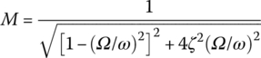
where F/K is the static deformation of the system under a static load F, as shown in Figure 2.44, and M is the dynamic magnification factor.
The frequency response curves of the system with forced damped vibration are plotted in Figure 2.46, which shows how M and α vary with Ω/ω. We call this the amplitude resonance when M is a maximum, which is the case for the excitation frequency ![]() . Then, for a lightly damped system, we have
. Then, for a lightly damped system, we have ![]() or
or ![]() . The condition at which F(t) and
. The condition at which F(t) and ![]() are in phase is called phase resonance, which occurs for
are in phase is called phase resonance, which occurs for ![]() when
when ![]() . It can be seen clearly from Figure 2.46 that for light damping the phase‐lag angle is very sensitive to frequency changes near
. It can be seen clearly from Figure 2.46 that for light damping the phase‐lag angle is very sensitive to frequency changes near ![]() , therefore this offers an ideal way to determine experimentally the phase‐resonance frequency ω.
, therefore this offers an ideal way to determine experimentally the phase‐resonance frequency ω.
Figure 2.46 Frequency response curves of forced damped vibration.
2.9.1.4 Steady‐state Vibration of a System with Structural Damping
The differential equation of motion of a lumped mass m is
For the steady‐state solution ![]() , we obtain
, we obtain
We obtain
where
Similar to viscous damping, phase resonance occurs for ![]() for a structural damping system. However, the amplitude resonance M of viscous damping systems occurs for
for a structural damping system. However, the amplitude resonance M of viscous damping systems occurs for ![]() , but is
, but is ![]() for a structural damping system when M also reaches its maximum. It is noteworthy and indicative of the physical shortcoming of the concept of structure damping that
for a structural damping system when M also reaches its maximum. It is noteworthy and indicative of the physical shortcoming of the concept of structure damping that ![]() for
for ![]() .
.
2.9.2 Complex Extended Transfer Matrix and Steady‐state Response
2.9.2.1 Complex Extended Transfer Matrix
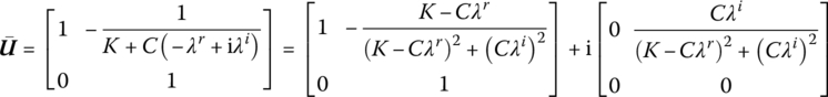
Now let us compute the steady‐state vibration of the system of Figure 2.44 using the MSTMM. The complex transfer matrix of the spring‐damper in parallel connection was found for the free vibrations in Equation (2.92), where λ is in the form of ![]() . If we consider steady‐state forced vibrations
. If we consider steady‐state forced vibrations ![]() and add an extra column to the transfer matrix, the extended transfer matrix relating the complex extended state vectors
and add an extra column to the transfer matrix, the extended transfer matrix relating the complex extended state vectors ![]() and
and ![]() is obtained:
is obtained:
Similarly, according to Equation (2.92) the extended transfer equation of a lumped mass is
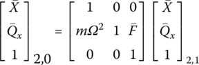
therefore the overall transfer equation of the system of Figure 2.44 is

Substituting the boundary conditions ![]() into the above formula yields
into the above formula yields
which coincides with Equation (2.132).
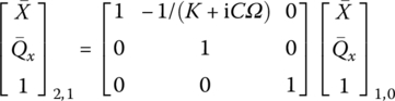
Two further examples of extended transfer matrices are given as follows. One is Equation (2.143) for a spring with stiffness K, shown in Figure 2.47a, and the other is Equation (2.144) for a damper with complex stiffness iCΩ, shown in Figure 2.47b. The elements of the state vectors have been written above the corresponding column of the transfer matrix.
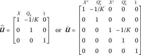
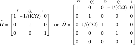
Figure 2.47 Spring and damper: (a) spring with stiffness K and (b) damper with complex stiffness iCΩ.
2.9.2.2 Steady‐state Response
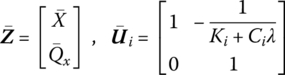
If we use the extended transfer matrices in their real form, as in Equation (2.95), the form of the extended state vector is

and the transfer equation is
The overall transfer matrix is obtained by multiplying the extended transfer matrix of each element in sequence:
where the overall transfer matrix ![]() still has the matrix form of Equation (2.145).
still has the matrix form of Equation (2.145).
Similar to the case for an undamped system, in the boundary state vectors of the damped system there are also m/2 components equal to zero. The beam is fixed at the input end and simply supported at the output end, so the corresponding boundary conditions are
The overall transfer equation can be expressed explicitly as
that is
This can be written as
so
Knowing the state vector ![]() at the input end, the other state vectors can be computed by the method described earlier.
at the input end, the other state vectors can be computed by the method described earlier.
Figure 2.48 Damping torsion system.
Table 2.15 Computation results of the forced damped vibration of the system
| Sequence number i | 1 | 3 | 5 | 7 |
|
|
0.2271 | 0.0908 | −0.1034 | −0.0801 |
|
|
0.3826 | 0.1530 | 0.4106 | 0.3191 |