
8
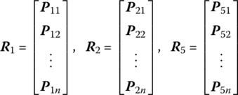
Discrete Time Transfer Matrix Method for Multi‐flexible‐body Systems
8.1 Introduction
Generally speaking, for many engineering problems, a dynamics model of a multi‐rigid‐body system (MRS) cannot meet the demand of engineering accuracy. For example, to implement the dynamic design required for precision firing of artillery and rocket launchers, the gun barrel and the guider of the rocket launcher have to be treated as elastic bodies to meet the demands of engineering accuracy [1, 249]. Therefore, the dynamics models of artillery systems and rocket launchers have to be treated as multi‐rigid‐flexible‐body systems (MRFSs). MRFSs are systems composed of rigid and flexible bodies undergoing large motion connected by various hinges. In MRFSs, not only are the elasticity and damping of connection points, as well as the large motion of body elements, considered, but also the coupling of deformation and large motion of the elements. The MRFS is the refinement, natural extension and further development of the physical model of the MRS. Using ordinary methods of multibody system dynamics, the derivation of the global dynamic equations of the MRFS is rather more complicated than those of the MRS, and the computational scale and cost are also greater, while the theory of MRFS dynamics is not as perfect that of MRS dynamics. How to establish the dynamic equations of general MRFSs and improve computational speed is one of the primary research directions in MRFS dynamics.
The description for the motion of a flexible body system can be divided into two categories: absolute and relative. Absolute description is related to the motion variables of each body under an inertial coordinate system. Relative description builds a local body‐fixed coordinate system for each body respectively, and decomposes the body motion into two parts: global motion of a rigid body along with the local body‐fixed coordinate system and deformation motion of a rigid body relative to the local body‐fixed coordinate system. The equations of motion can be established directly by using these two motion variables. A flexible body has infinite degrees of freedom (DOFs), and there are some methods to deal with elastic deformation in multibody system dynamics, such as the Rayleigh–Ritz method, the finite segment method, the finite element method (FEM) and the modal analysis method. There are various ways to select the generalized coordinates of a multibody system, including the hybrid coordinate approach, the corotational coordinate approach and the absolute nodal coordinate approach.
Based on the discrete time transfer matrix method for multibody systems (MSDTTMM), as introduced in Chapter 7, this chapter introduces the discrete time transfer matrix method (DTTMM) for an MRFS [61, 69–73], including dynamic equations, state vectors, transfer equations and transfer matrices of planar and spatial flexible bodies, transfer matrices of various hinges, the algorithm and examples of the DTTMM for the MRFS. The results indicate that the DTTMM for the MRFS is not only valid for the dynamics of the MRFS, but also very efficient due to the following features: no need for global dynamics equations of the system and high computational speed.
8.2 Dynamics of a Flexible Body with Large Motion
In rigid body dynamics, the general motion of a rigid body can be decomposed into the translation of the body‐fixed coordinate system and the relative rotation of the body‐fixed coordinate system with respect to its origin. To eliminate the inertia coupling between the translation and rotation at the acceleration, the principal axes of inertia of the rigid body are selected as the body‐fixed coordinate system to produce the inertial tensor in diagonal form. When the flexible body moves, the relative positions of all points of the body are time‐varying and its motion is described exactly using the continuum mechanics method. Usually, we cannot use one uniform body‐fixed coordinate system and for each flexible body we use one floating frame or floating coordinate system described by the Cartesian coordinate system. The origin and the orientation of coordinate axes of the floating coordinate system are time‐varying with respect to the flexible body. The principles of choosing the floating frame are not only to try to reduce or eliminate the coupling between the overall motion of the flexible body and relative deformation motion in order to decouple the equations of motion, but also to linearize the relative deformation motion of the flexible body and describe the relative deformation motion by a first‐order function.
8.2.1 Kinematics of a Flexible Body
Using the floating frame of reference formulation, the translational motion is described by body‐fixed coordinate system o1x1y1z1, which is parallel to the inertia coordinate system, and the large rotation is described by body‐fixed coordinate system O2x2y2z2, which takes o1 as the origin. The motion of a flexible body can be decomposed into the large motion of the body‐fixed coordinate system and the motion of deformation with respect to the body‐fixed coordinate system.
The schematic decomposition diagrams of the motion of a flexible body, from position 1 to position 4, are shown in Figure 8.1. First, the flexible body is assumed to be a rigid body, and the initial position 1 translates to 2, then rotates to 3 around an arbitrary point on the flexible body. The flexible body finally undergoes deformation motion to position 4. As shown in Figure 8.2, the position vector of arbitrary point j on the flexible body can be expressed as
where rj is the position vector of an arbitrary point j on the flexible body with respect to the inertia coordinate system and ![]() is the position vector of the origin of body‐fixed coordinate system with respect to the origin of the inertia coordinate system.
is the position vector of the origin of body‐fixed coordinate system with respect to the origin of the inertia coordinate system. ![]() is the position vector of point j on the flexible body with respect to the origin of the body‐fixed coordinate system.
is the position vector of point j on the flexible body with respect to the origin of the body‐fixed coordinate system.
Figure 8.1 Decomposition of flexible body motion.
Figure 8.2 Position description of an arbitrary point on a flexible body.
![]() can be decomposed into the undeformed position vector
can be decomposed into the undeformed position vector ![]() and the deformable vector uj
and the deformable vector uj
therefore
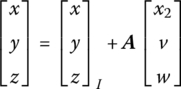
For a flexible body with large planar motion, projecting Equation (8.3) onto the inertia coordinate system yields
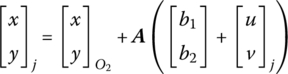
where

A is the transformation matrix of planar motion, and ![]() and
and ![]() are the column matrices of
are the column matrices of ![]() and uj, respectively, in the body‐fixed coordinate system.
and uj, respectively, in the body‐fixed coordinate system.
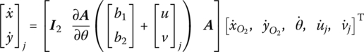
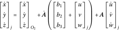
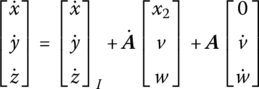
Differentiating Equation (8.4) with respect to time, the absolute velocities of point j on the flexible body can be obtained
where

Hence Equation (8.6) can be written as
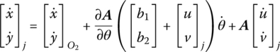
or
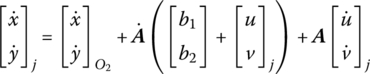
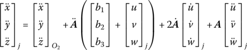
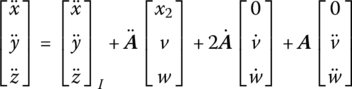
Differentiating Equation (8.4) twice with respect to time, the absolute accelerations of point j on a flexible body are as follows
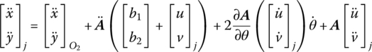
According to Equation (8.7),
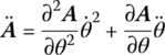
where

therefore
Thus Equation (8.11) can be rewritten as

It is clear that the first term on the right‐hand side of Equation (8.15) is the average translation acceleration of the flexible body, the second term is the normal acceleration of rotation, the third term is the tangent acceleration of rotation, the fourth term is Coriolis acceleration and the fifth term is relative deformation acceleration.
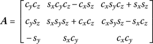
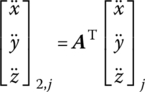
Similarly, for an elastic body with large spatial motion, by projecting Equation (8.3) onto the inertia coordinate system and differentiating it with respect to time, the positions, absolute velocities and absolute accelerations of point j on a flexible body can be obtained:

where ![]() and
and ![]() are coordinate column matrices of
are coordinate column matrices of ![]() and uj, respectively, in the body‐fixed coordinate system. A is the transformation matrix of the coordinate system. For an element with large spatial motion, we obtain
and uj, respectively, in the body‐fixed coordinate system. A is the transformation matrix of the coordinate system. For an element with large spatial motion, we obtain
8.2.2 Discretization and Generalized Coordinates of a Flexible Body
After the dynamic equations of planar motion of a flexible body with elastic deformation have been derived, the transfer matrix of a flexible body can be developed. The motion of the flexible body is determined by two groups of generalized coordinates which describe the motion of the reference coordinate system and the elastic deformation. The translation and rotation of the floating frame of the flexible body are described in the generalized coordinates of the body‐fixed coordinate system, and the deformation of the flexible body with respect to the body‐fixed coordinate system are described using the generalized coordinates of elastic deformation. There are several methods describing the deformation of an elastic body [242].
Rayleigh–Ritz method
The assumed displacement field, which satisfies the compatibility and completeness, is constructed for an elastic body. The assumed displacement field is described by Ψ(x, y, z), which describes the deformation of the elastic body and can be partitioned as ![]() . The deformation of each point on the body u can be expressed as
. The deformation of each point on the body u can be expressed as
where Q(t) are the generalized coordinates of elastic deformation.
This is the most basic method for the approximation of the deformation of a continuous body in elastic mechanics. For complex shape, boundary and load, it is extremely difficult to construct a displacement field that is suitable for the entire flexible body.
Finite element method
This method is a kind of piecewise Rayleigh–Ritz method. Its basic idea is to discretize the continuous body into a group of finite elements which connect with each other according to a certain mode. Because the elements can be assembled with different connections and may have different shapes, FEM can formulate the body with complex shape, boundary and load.
By the rapid development of computer performances, FEM has become a powerful tool to analyze and compute engineering structures and general elastic bodies. When the actual object is simulated approximately using FEM, displacement of infinite particles on the elastic body is described by the shape function of the finite element node displacements. Deformation uj of an arbitrary point on element j of the body can be expressed as
where Nj is the deformation pattern of element j (or assumed displacement field), which is called the shape function of element j, and ![]() is the node displacement of the element.
is the node displacement of the element.
After assembling all the elements, the displacements of all the nodes construct generalized coordinates of the elastic body. The infinite DOFs of modeling can be reduced into finite DOFs of modeling using FEM. Usually, the remaining number of DOFs is still considerably large to guarantee the computational precision.
Component mode synthesis method
In structure dynamic analysis, the displacement (deformation) of an object which changes with time is often described using its mode coordinates, that is
where ![]() is the mode matrix, Q(t) are generalized coordinates and n is the mode number.
is the mode matrix, Q(t) are generalized coordinates and n is the mode number.
The advantages of the component mode synthesis method are:
- The computational scale could be reduced by the modal truncation according to aprioristic response characteristics and required precision. In some cases, low‐order modes have more contribution to the response, for example some elastic mechanical arms can take the first one or two modes and satellite solar panels usually need to take the first five or six modes. For a fluid–solid coupling system, where high‐order modes play an important role, we could also truncate off the less contributive modes to maximally reduce the solution scale.
- The mode synthesis technique makes it more convenient to study the vibration of a large‐scale complex system.
- The results of the mode test are applied directly, so the theory and numerical analysis closely integrate with the experimental data.
8.2.3 Dynamic Equations of a Flexible Body with Large Planar Motion
There are some basic assumptions in linear elasticity mechanics:
- Continuity assumption. The volume of the entire object is filled with the mediums which compose this object, without any space.
- Entire elasticity assumption. The object completely obeys Hooke’s law, that is, strain is directly proportional to the stress components which cause the strain, namely, the elastic constant does not change with the stress components or strain components.
- Homogeneity assumption. The entire object is composed of identical material.
- Isotropy assumption. The characteristics of the object in each direction are all the same, that is to say elastic constant does not change with direction.
- Small deformation assumption. Suppose that each deformation is far smaller than the original size of the object, namely the strain is far smaller than 1, therefore when we establish the balance equation after object deformation, we may use the size before the deformation to replace the size after the deformation without causing appreciable error.
The planar and spatial dynamic equations of an elastic body can be derived on the basis of these five assumptions.
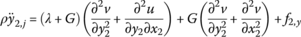
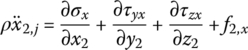
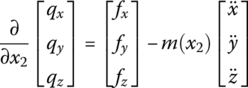
The force analysis of infinitesimal element of an elastic body with large planar motion is shown in Figure 8.3a. Projecting the absolute acceleration of an arbitrary point j on the elastic body to body‐fixed coordinate system O2x2y2, this yields

Figure 8.3 Force analysis of an infinitesimal element of an elastic body: (a) force analysis of an infinitesimal element of a planar elastic body and (b) force analysis of an infinitesimal element of a spatial elastic body.
According to Newton’s second law,

which can be simplified as
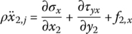
Similarly,
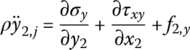
where σ and τ are normal stress and shear stress, respectively, and their directions are distinguished by the subscripts (Figure 8.3a). f2,x is the distribution of external force and ρ is area mass density per unit surface. The subscript 2 denotes variables in body‐fixed coordinate system O2x2y2.
According to elasticity mechanics, the constitutive equation of planar isotropic linear elastic material, that is, generalized Hooke’s law, can be written as
where λ is the Lamé constant, ![]() ,
, ![]() , E is Young’s modulus and μ is Poisson’s ratio. ε and γ are normal strain and shear strain, respectively.
, E is Young’s modulus and μ is Poisson’s ratio. ε and γ are normal strain and shear strain, respectively.
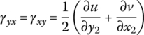
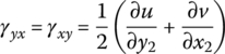
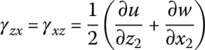
The kinematic equations of small deformation and isotropic linear elastic material are
Substituting Equations (8.27) to (8.32) into Equations (8.25) and (8.26), we obtain

The dynamic equations of flexible body deformation with large planar motion are Equations (8.33) and (8.34). These are different from the dynamic equations of a planar elastic body with small displacement. Here, the acceleration expression includes not only the deformation acceleration, but also the characteristic quantity of the motion of a body‐fixed coordinate system, such as the angular acceleration of the body‐fixed coordinate system.
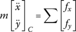
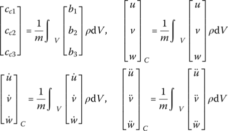
Because the motion of a flexible body is described by the large motion of a floating frame and the deformation relative to the moving reference frame, respectively, we should take into account the equations governing the motion of the floating frame of reference. Assume mid‐point j in Equation (8.15) is mass center C of the flexible body, hence,

where

The mass center motion equation of the flexible body with large planar motion becomes
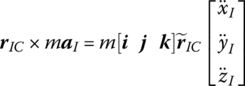
Setting the origin O2 of the body‐fixed coordinate system to be the momentum center, using the theorem of the absolute angular momentum of the particle system with respect to the moving momentum center yields
where ![]() is the absolute moment of momentum of the flexible body of large planar motion with respect to point O2.
is the absolute moment of momentum of the flexible body of large planar motion with respect to point O2. ![]() is the radius vector of mass center C of the flexible body with respect to point O2. m is the mass of the flexible body,
is the radius vector of mass center C of the flexible body with respect to point O2. m is the mass of the flexible body, ![]() is the acceleration of point O2 and M is the principal moment of the external forces.
is the acceleration of point O2 and M is the principal moment of the external forces.
In the body‐fixed coordinate system O2x2y2,
Rearranging Equation (8.38), this becomes
8.2.4 Dynamic Equations of a Flexible Body with Large Spatial Motion
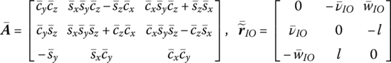
Similar to the derivation of the dynamic equations of a flexible body with large planar motion, the force analysis of an infinitesimal element of a flexible body with large spatial motion is shown in Figure 8.3b. Projecting the absolute acceleration of an arbitrary point j on the flexible body to the body‐fixed coordinate system O2x2y2z2, we obtain
where A is the transformation matrix of the coordinate system, which is shown in Equation (8.19).
According to Newton’s law of motion, we obtain
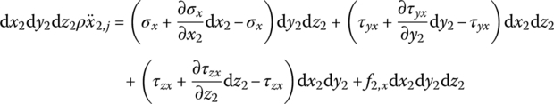
This can be simplified to
Similarly, for the y2 and z2 directions we obtain


where σ and τ are the normal stress and shear stress, and their directions are distinguished by the subscripts (Figure 8.3b). f2,x, f2,y and f2,z are the distributed external forces components, respectively, ρ is the mass density and subscript 2 denotes parameters expressed in the body‐fixed coordinate system O2x2y2z2.
According to the theory of elasticity, the constitutive equations of three‐dimensional isotropic linear elastic materials can be written as:
The kinematics equations of an isotropic linear elastic material for small deformation are

Substituting Equations (8.45) to (8.56) into Equations (8.42) and (8.44), we obtain


The dynamic equations of the deformation of a flexible body with large spatial motion are defined by Equations (8.57) to (8.59). Similar to Equations (8.33) and (8.34), the acceleration expressions given by Equations (8.57) to (8.59) include the deformation acceleration and the characteristic quantity of the motion of the body‐fixed coordinate system.
Similar to the derivation of the equation of motion of the mass center of a flexible body with large planar motion, mid‐point j in Equation (8.18) is assumed to be the mass center C of a flexible body, therefore
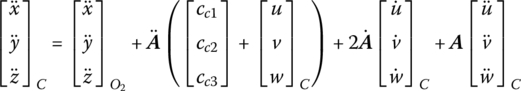
where
The mass center motion equation of a flexible body moving in space is
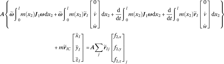
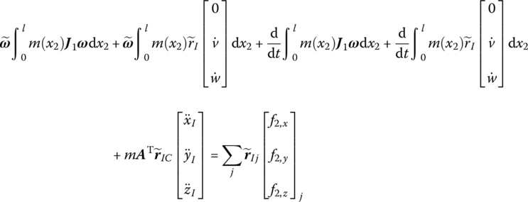
Let the origin O2 of the body‐fixed coordinate system be the moment center. Using the theorem of the absolute angular momentum of a particle system with respect to the moving moment center, the rotational equation of a flexible body with large spatial motion is
where ![]() is the absolute momentum moment of the flexible body with large spatial motion with respect to point O2. The meanings of the other terms are the same as in Equation (8.37).
is the absolute momentum moment of the flexible body with large spatial motion with respect to point O2. The meanings of the other terms are the same as in Equation (8.37).
8.3 State Vector, Transfer Equation and Transfer Matrix
The definition of a state vector of a rigid body in the MRFS is the same as in the DTTMM for an MRS, as developed in Chapter 7. For the definition of the state vector of a flexible body, the physical variables that reflect the relative deformation of a flexible body must be considered in addition to the state variables in the state vectors of a rigid body. The deformation of a flexible body is described using the modal analysis method and the deformation of an arbitrary point on the flexible body, which is a function of time, can be described by generalized coordinates corresponding to eigenvectors. Therefore, by the addition of generalized coordinates which describe the deformation of a flexible body to the definition of the state vector of a rigid body, the state vector of a flexible body can be obtained.
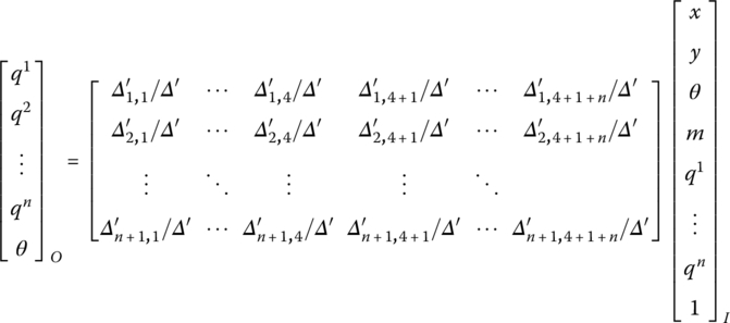
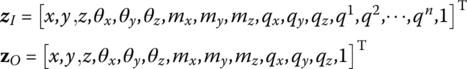
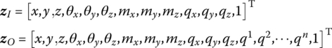
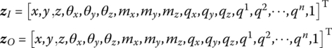
The state vector of a flexible body moving in a plane is
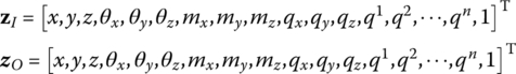
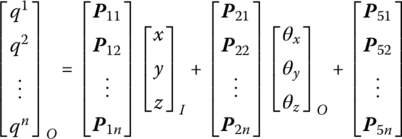
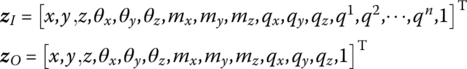
The state vector of a flexible body moving in space is
where x, y, z, θx, θy, θz and mx, my, mz, qx, qy, qz are similar to the terms in the state vectors of a rigid body, while x, y, z, θx, θy and θz are the position coordinates of the origin and its orientation angles of the floating frame, respectively. mx, my, mz, qx, qy and qz are the internal moments and internal forces projected to x, y and z, respectively. ![]() are the generalized coordinates which describe the deformation using the modal analysis method, and the superscript n is the highest order of the modes.
are the generalized coordinates which describe the deformation using the modal analysis method, and the superscript n is the highest order of the modes.
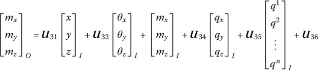
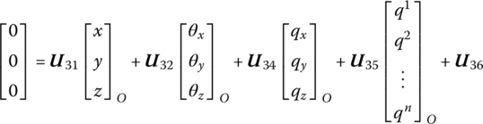
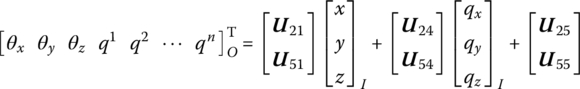
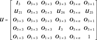
Similar to the DTTMM for MRSs, by linearization of the dynamic equations of the flexible body element the transfer equation which connects the different connection points of a flexible body is
where the transfer matrix U at the current time is known or can be obtained by iterative computation.
Compared with the DTTMM for MRSs, the DTTMM for MRFSs has a similar approach, but there are two important differences:
- The deformation effect of flexible body must be considered in the DTTMM for an MRFS, therefore the state vector and transfer matrix of a flexible body have generalized coordinates which describe the deformation and its correlated terms with respect to the state vector and transfer matrix of a rigid body.
- In an MRS, the body and hinge have the same number of state variables (at least as a chain system), but in an MRFS the state vector of the hinge is determined by the characteristics and transfer direction of the two ends of the hinge. Readers should pay attention to these differences, which will be seen in Section 8.5.
8.4 Transfer Matrix of a Beam with Large Planar Motion
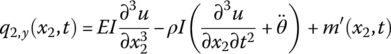
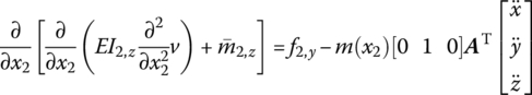
Using the description of the deformation and dynamic equations of motion of a flexible body in Section 8.2, the dynamic equations of a Euler–Bernoulli beam can be obtained:

where u is the transverse deformation of the beam, l is the length of the beam, ![]() is the mass per unit length and m is the mass of the beam,
is the mass per unit length and m is the mass of the beam, ![]() . f2,x(x2, t) and f2,y(x2, t) are the distributed external forces acting on the beam projected to x2 and y2, respectively, and
. f2,x(x2, t) and f2,y(x2, t) are the distributed external forces acting on the beam projected to x2 and y2, respectively, and ![]() is the sum of moments of all the forces and the moment acting on the beam with respect to point O2.
is the sum of moments of all the forces and the moment acting on the beam with respect to point O2.
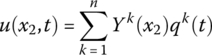
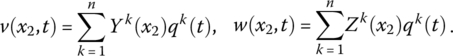
By the modal analysis method, the mode shapes of the component with small deformation, which satisfy the boundary condition, can be obtained directly. Using the modal analysis method, the transverse deformation u of the beam in Equations (8.66) to (8.68) can be expressed as

Using the finite‐order mode shape to describe the solution of the system, for example let ![]() ,
,
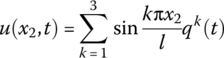
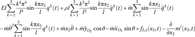
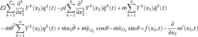
Substituting Equation (8.70) into Equation (8.67), integrated along the axial direction of the Euler–Bernoulli beam with uniform cross‐section, this yields
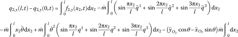
namely
Substituting Equations (8.27) and (8.28) into Equation (8.72) and rearranging yields
Similarly, from Equation (8.68),
Equations (8.73) and (8.74) can be rewritten as
where
Discretizing Equation (8.66) gives
Equation (8.77) can be rewritten as
where

If the distributed external force acting on the beam is f, and the distributed external moment is m′, then

For small deformation, eliminating the moment  , which is caused by axial distributed force, yields

Substituting Equation (8.81) into Equation (8.78) yields
Substituting Equation (8.75) into Equation (8.82) yields
As ![]() , then
, then

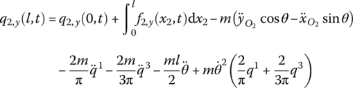
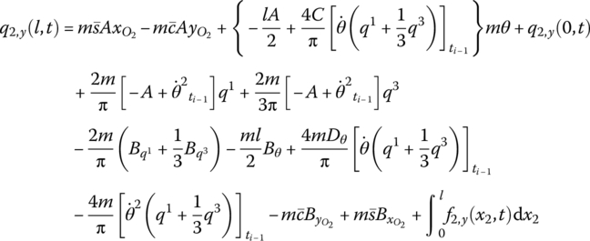
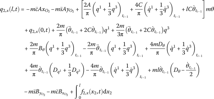
Projecting Equations (8.75) and (8.76) to the inertia coordinate system, we obtain
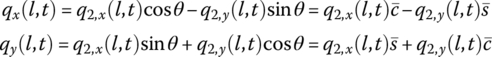
Then

namely
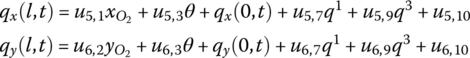
The derivation of state variables x(l, t), y(l, t) and θ(l, t) with respect to the body‐fixed coordinate system is the same as that of a rigid body with one input end and one output end.
The state vector of the planar beam can be defined as
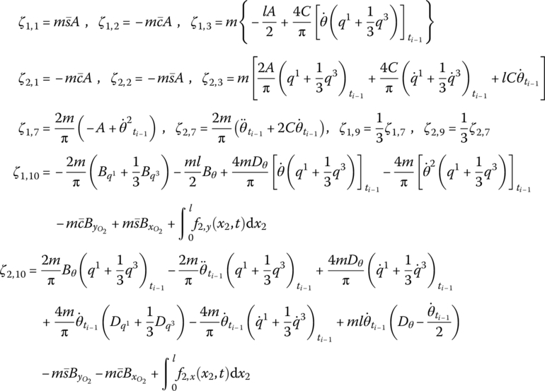
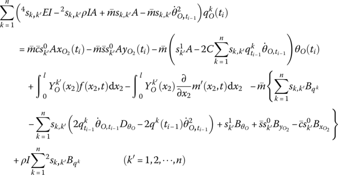
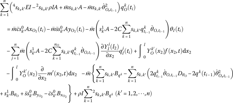
From Equation (8.88), considering that the generalized coordinates of the two ends of the beam are equal, the transfer equation of the planar Euler–Bernoulli beam with large motion yields
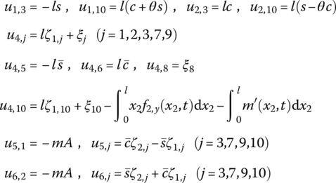
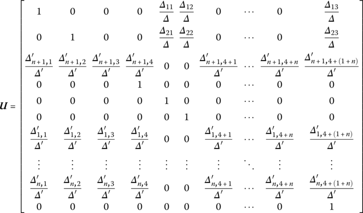
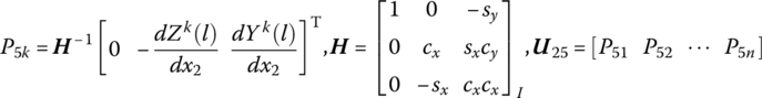
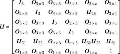
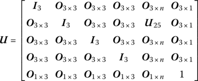
The transfer matrix is
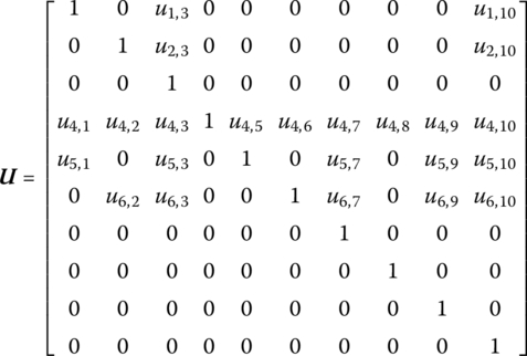
where
8.5 Transfer Matrices of Smooth Hinges Connected to a Beam with Large Planar Motion
The transfer matrices and state vectors of the hinges of MRFSs are determined by the characteristics and transfer direction of the connected bodies, which are different from those in MRSs. There are four kinds of smooth hinges: (1) the outboard body and the inboard body are both rigid, (2) the inboard body is flexible and the outboard body is rigid, (3) the inboard body is rigid and the outboard body is flexible, and (4) both the outboard body and the inboard body are flexible. The transfer matrices of smooth hinges whose outboard body is a beam or rigid body are discussed in the following sections.
8.5.1 Smooth Hinges whose Outboard Body is a Beam
The transfer matrices of smooth hinges whose outboard body is a beam and inboard body is a beam or rigid body are derived as follows. Because x, y, qx and qy in the two ends of smooth hinge are equal, and m is zero, we only need to determine θ and ![]() of the output end of the smooth hinge.
of the output end of the smooth hinge.
According to the rotation equation of the beam element, we obtain
Substituting this equation into Equation (8.67), the vibration equation of the beam is

Substituting Equation (8.70) into Equation (8.91) yields
Multiplying both sides of Equation (8.92) by ![]() (
(![]() ) and integrating along x2 gives
) and integrating along x2 gives

Let
where u4,1, u4,2, ![]() , u4,10 are the elements of the transfer matrix of the outboard beam.
, u4,10 are the elements of the transfer matrix of the outboard beam.
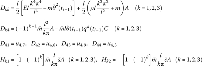
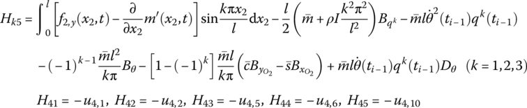
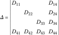
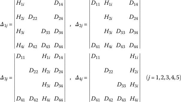
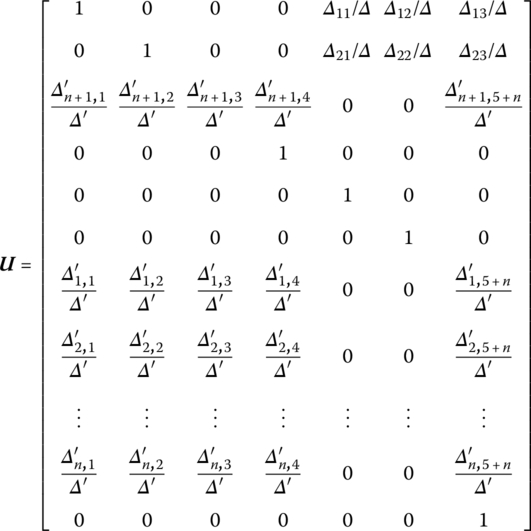
Linearizing Equation (8.93) yields
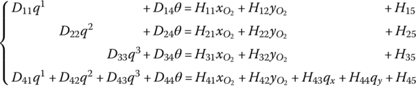
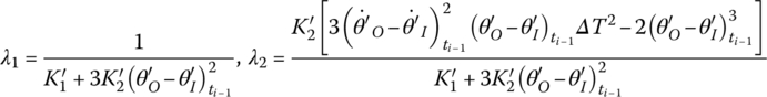
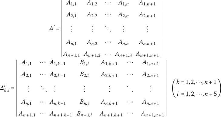
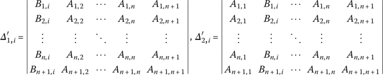
Using the Cramer rule yields

where
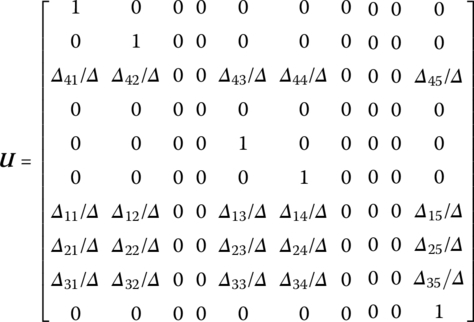
To reduce computational cost, we usually do not use the Cramer rule to solve the linear equations. Instead, we simplify Equation (8.94) with transformations to make the coefficient matrix on the left‐hand side of the equation into a unit matrix and obtain Equation (8.98).
For a smooth hinge whose outboard body is a beam, the transfer matrices are deduced for two cases: the inboard body is a beam and the inboard body is a rigid body. The deduction is accomplished based upon an assumption that the output end of the outboard body is also connected with another smooth hinge. If the output end of the outboard body is not connected with another smooth hinge, we can deduce the transfer matrices in a similar way.
8.5.1.1 Smooth Hinge whose Outboard and Inboard Bodies are Beams
If the highest order of the modes ![]() , the state vectors of the input and output ends of the smooth hinge whose inboard and outboard bodies are beams are defined respectively as
, the state vectors of the input and output ends of the smooth hinge whose inboard and outboard bodies are beams are defined respectively as
The transfer equation is
The transfer matrix is
8.5.1.2 Smooth Hinge whose Outboard Body is a Beam and whose Inboard Body is a Rigid Body
For a smooth hinge whose outboard body is a beam and whose inboard body is a rigid body, the transfer matrix of the smooth hinge can be obtained by eliminating the columns corresponding to the generalized coordinates in Equation (8.98). The state vectors of the input and output ends of this smooth hinge are, respectively,
The transfer equation is
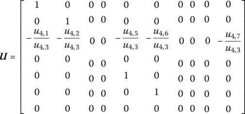
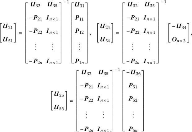
Eliminating columns 7–9 in Equation (8.98), the transfer matrix of this smooth hinge is

8.5.2 Smooth Hinge whose Outboard Body is a Rigid Body
8.5.2.1 Smooth Hinge whose Inboard Body is a Rigid Body
The smooth hinge whose outboard and inboard bodies are rigid is discussed in Chapter 7. The state vectors of the input and output ends of the smooth hinge whose outboard and inboard bodies are rigid are defined respectively as
The transfer matrix is Equation (7.219).
8.5.2.2 Smooth Hinge whose Inboard Body is a Beam
The derivation of the transfer matrix of smooth hinge whose outboard body is a rigid body and whose inboard body is a beam is the same as Equation (7.219). The state vectors of the input and output ends of this smooth hinge are defined respectively as
The transfer equation is
Inserting three columns with zero elements behind the sixth column in Equation (7.219), the transfer matrix of this smooth hinge can be obtained:
The meanings of the elements in this equation are the same as in Equation (7.219).
8.6 Transfer Matrices of Spring Hinges Connected to a Beam with Large Planar Motion
Similarly to the smooth hinges connected to a beam with large planar motion introduced in section 8.5, there are four kinds of spring hinges connected to a beam with large planar motion: (1) both of the outboard and inboard bodies are rigid, (2) the inboard body is flexible and the outboard body is rigid, (3) the inboard body is rigid and the outboard body is flexible, and (4) both the outboard and inboard bodies are flexible. The transfer matrix of the spring hinge whose outboard and inboard bodies are rigid bodies with planar motion was given in Chapter 7. Here the transfer matrix of a spring hinge connected to a flexible body with planar motion is discussed.
8.6.1 Dynamic Equation of a Spring Hinge Connected to a Beam with Planar Motion
Similarly to section 7.6, the spring hinge includes a linear (or nonlinear) spring and a torsional spring.
The mass of the spring is omitted. According to Equations (7.200) and (7.201), we obtain
The variables are the same as in section 7.6.1.
For a nonlinear torsional spring,
where
![]() and
and ![]() are the stiffness coefficients of a nonlinear torsional spring,
are the stiffness coefficients of a nonlinear torsional spring, ![]() and
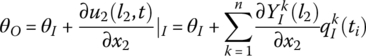
and ![]() are the orientation angles of the input and output ends of the torsional spring, respectively, θI and θO are the orientation angles of the inboard and outboard bodies of the torsional spring, respectively, and
are the orientation angles of the input and output ends of the torsional spring, respectively, θI and θO are the orientation angles of the inboard and outboard bodies of the torsional spring, respectively, and ![]() and
and ![]() are rotation angles caused by the deformation of the inboard and outboard bodies of torsional spring. If the inboard or outboard body of the torsional spring is rigid, then
are rotation angles caused by the deformation of the inboard and outboard bodies of torsional spring. If the inboard or outboard body of the torsional spring is rigid, then ![]() or
or ![]() .
.
Linearizing Equation (8.108) yields
where
For the massless spring and the massless torsional spring, Newton’s third law of motion tells us that
8.6.2 Transfer Matrix of a Spring Hinge whose Inboard and Outboard Bodies are Beams moving in a Plane
For a spring hinge whose inboard and outboard bodies are beams moving in a plane, it is necessary to determine the relation between the angular orientation θ and the generalized coordinates ![]() of the output end of the spring hinge and the state vector of the input end. Using the modal expansion, the transverse deformation u of a beam becomes
of the output end of the spring hinge and the state vector of the input end. Using the modal expansion, the transverse deformation u of a beam becomes
Substituting Equation (8.112) into the equation of vibration Equation (8.91) of the outboard beam, we obtain
Let

Multiplying both sides of Equation (8.113) by ![]() (
(![]() ) and integrating along x2, we obtain
) and integrating along x2, we obtain
Linearizing Equation (8.115) yields

Substituting Equation (8.112) into Equation (8.110) yields
Let
where ![]() .
.
The x, y and m of the two ends of the state vectors of the spring hinge are equal.
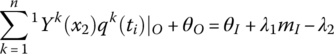
Solving Equation (8.118) for the state variables θ and ![]() of the output end in terms of the state variables x, y, θ, m and qk of the input end and applying the Cramer rule for simplicity, we obtain
of the output end in terms of the state variables x, y, θ, m and qk of the input end and applying the Cramer rule for simplicity, we obtain
where
For example,
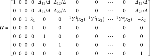
Therefore, the transfer equation of a spring hinge whose inboard and outboard bodies are beams is
where the definition of the state vectors is the same as for the state vectors of the beam, that is
The transfer matrix is
8.6.3 Transfer Matrix of a Spring Hinge whose Inboard Body is Rigid and whose Outboard Body is a Beam moving in a Plane
If the inboard body of a spring hinge is rigid body, according to the above analysis we know ![]() and according to Equation (8.117) this becomes
and according to Equation (8.117) this becomes
Similarly, combining Equations (8.116) and (8.122), let θ and ![]() in the state vector of the spring hinge output end be expressed as a linear representation of x, y, θ, m and qk in the state vector of the input end. Using the Cramer rule, the transfer matrix of a spring hinge whose inboard body is rigid and whose outboard body is a beam moving in plane can be obtained. The state vectors of the input and output points of this spring hinge are
in the state vector of the spring hinge output end be expressed as a linear representation of x, y, θ, m and qk in the state vector of the input end. Using the Cramer rule, the transfer matrix of a spring hinge whose inboard body is rigid and whose outboard body is a beam moving in plane can be obtained. The state vectors of the input and output points of this spring hinge are
The transfer equation is
The transfer matrix is
where the meaning of all the elements is the same as in Equation (8.121), except that we let ![]() during the computation.
during the computation.
8.6.4 Transfer Matrix of a Spring Hinge whose Inboard Body is a Beam and whose Outboard Body is a Rigid Body Moving in Plane
If the outboard body of spring hinge is a rigid body, according to the above analysis we know ![]() , and according to Equation (8.117)
, and according to Equation (8.117)

Similarly, combining Equations (8.106), (8.107), (8.111) and (8.126), the transfer matrix of a spring hinge whose inboard body is a beam and whose outboard body is a rigid body moving in a plane can be obtained.
The state vectors of the input and output ends of a spring hinge whose inboard body is beam and whose outboard body is a rigid body moving in a plane are
The transfer equation is
The transfer matrix is
8.7 Transfer Matrix of a Fixed Hinge Connected to a Beam
There are three kinds of fixed hinges connected to a beam moving in a plane: (1) both the outboard and inboard bodies are flexible, (2) the outboard body is flexible and the inboard body is rigid, and (3) the outboard body is rigid and the inboard body is flexible.
8.7.1 Transfer Matrix of a Fixed Hinge whose Inboard and Outboard Bodies are Beams Moving in a Plane
For a fixed hinge whose inboard and outboard bodies are Euler–Bernoulli beams moving in a plane, its position coordinates, internal forces and internal moments are equal at the input and output ends. The relation between θ of the output end and ![]() of the state vectors of input end needs to be derived.
of the state vectors of input end needs to be derived.
For a fixed hinge whose inboard and outboard bodies are beams moving in a plane, the relation of orientation angles at the input and output ends is
where θI and θO are the orientation angles of the fixed hinge at the input and output ends, respectively. ![]() is the rotation angle caused by the deformation of inboard beam,
is the rotation angle caused by the deformation of inboard beam, ![]() and
and ![]() are the mode shape function and generalized coordinates that describe the deformation of inboard beam, and the superscript n is the highest order of the modes. If the inboard body is rigid, then
are the mode shape function and generalized coordinates that describe the deformation of inboard beam, and the superscript n is the highest order of the modes. If the inboard body is rigid, then ![]() .
.
Similar to section 8.6.2, the transverse deformation u of the beam can be expressed by modal superposition. Substituting it into the vibration equation of the outboard Euler–Bernoulli beam, integrating along axial direction and linearizing, we obtain
where θO is the orientation angle of the fixed hinge at the output end, that is, the rotation angle of the body‐fixed coordinate system of its outboard beam. ![]() and
and ![]() are the mode shape function and generalized coordinates describing the deformation of the outboard beam. The meanings of the other elements are the same as in Equation (8.116).
are the mode shape function and generalized coordinates describing the deformation of the outboard beam. The meanings of the other elements are the same as in Equation (8.116).
Substituting Equation (8.130) into Equation (8.131) gives
Let

then
The transfer equation of the fixed hinge whose inboard and outboard bodies are beams moving in a plane is denoted as
The state vectors are
The transfer matrix is

where
8.7.2 Transfer Matrix of a Fixed Hinge whose Inboard Body is a Rigid Body and whose Outboard Body is a Beam
For a beam with transverse vibration fixed on the rigid body, the position coordinates, orientation angles, internal forces and internal moments of the fixed hinge are equal at its input and output ends. Similar to section 8.5, but eliminating columns corresponding to generalized coordinates which describe the deformation of the inboard beam in Equation (8.135), the transfer equation of the fixed hinge whose inboard body is a rigid body and whose outboard body is a beam is
The state vectors are
The transfer matrix is
where the meaning of all elements is the same as in Equation (8.135).
8.7.3 Transfer Matrix of a Fixed Hinge whose Inboard Body is a Beam and whose Outboard Body is a Rigid Body
The derivation of the transfer matrix of a fixed hinge whose inboard body is a beam and whose outboard body is rigid is the same as in section 8.5, except some rows in Equation (8.135) corresponding to the generalized coordinates which describe the deformation of the outboard beam need to be eliminated.
The transfer equation and transfer matrix of the fixed hinge whose inboard body is beam and whose outboard body is rigid can be obtained as
The state vectors are
The transfer matrix is

where the meaning of all elements is the same as in Equation (8.135).
8.8 Dynamics Equation of a Spatial Large Motion Beam
The Euler–Bernoulli beam theory assumptions are:
- The cross‐section of the beam which is perpendicular to the central line before deformation doesn’t distort after the deformation (rigid cross‐section hypothesis).
- The cross‐section after the deformation is still perpendicular to the axis after the deformation. The distributed load acting on the beam includes the distributed external force f, the distribution inertia force f ′ and the distributed moment
 .
.
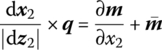
For the spatial beam shown in Figure 8.4, based on the equilibrium condition of forces

Figure 8.4 Model of a beam element.
Based on the equilibrium condition of moment acting on the output end of the element, we have
Neglecting the second‐order small quantities and according to Equations (8.140) and (8.141), we obtain
The geometric relationship of the beam element is
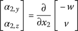
where v and w are the components of deformation of an arbitrary point on the central line of the beam along axes y2 and z2, respectively. α2,y and α2,z are components of the rotation angle caused by beam deformation along axes y2 and z2, respectively.
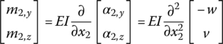
According to material mechanics,
As shown in Figure 8.5, oxyz is the inertia coordinate system and O2x2y2z2 is the body‐fixed coordinate system of the beam, whose origin is fixed on one end of the beam. The coordinate axis O2x2 and the direction of the axis of the undeformed beam coincide. The motion of the beam can be decomposed into rigid motion and deformation motion. Here, the undeformed position is the position when the beam only undergoes rigid motion without deformation.
Figure 8.5 Body‐fixed coordinate system of a beam.
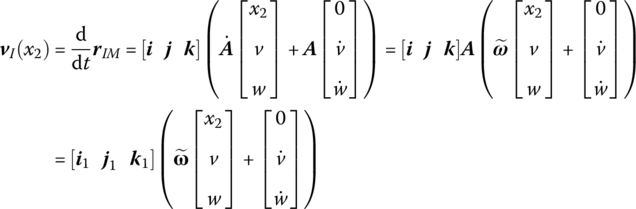
The coordinates of an arbitrary point of the beam in the inertia coordinate system oxyz are
From Equation (8.146), the absolute velocity and absolute acceleration of this point are
Projecting Equation (8.142) to the inertia coordinate system leads to
Substituting Equation (8.145) into Equation (8.143), we obtain


Substituting Equations (8.150) and (8.151) into Equation (8.142), the transverse vibration equations of the beam, yields

The theorem of the absolute angular momentum of a particle system with respect to the moving point is
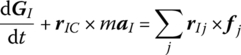
where
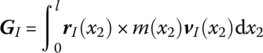

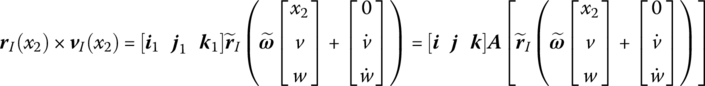
GI is the absolute moment of momentum of a particle system with respect to the input end I, (i, j, k) are three base vectors of the inertia coordinate system and (i1, j1, k1) are three base vectors of the body‐fixed coordinate system.
Substituting Equation (8.158) into Equation (8.155), in the inertia coordinate system, gives
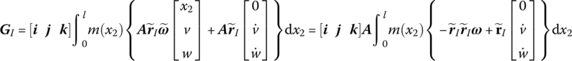
therefore
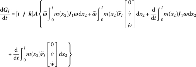
where
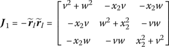
In the inertia coordinate system, ![]() can be expressed as
can be expressed as
where
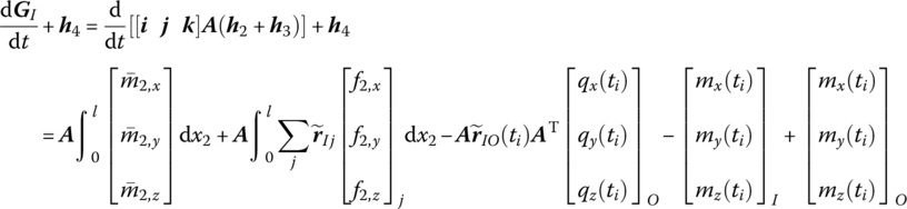
Substituting Equations (8.160) and (8.162) into Equation (8.154), the rotation equations of the beam in the inertia coordinate system can be found:
Using the transformation matrix, the rotation equations of the beam in the body‐fixed coordinate system can be obtained:
8.9 Transfer Matrix of a Spatial Large Motion Beam
Consider the transverse vibration of a Euler–Bernoulli beam with large spatial motion. The state vector is defined as
For the uniform beam with uniform cross‐section ![]() , the length of the beam is l and the mass is
, the length of the beam is l and the mass is ![]() .
.
Let
and combine Equations (8.27) and (8.28) as
In the inertia coordinate system, considering Equation (8.146) and integrating Equation (8.149) in the limit [0, l], we obtain

Let
Then
Substituting Equations (8.172) and (8.171) into Equation (8.170) and rearranging it yields

where
Linearize the rotation equation of the beam in the inertia coordinate system and let
From Equation (8.154), if the beam is only excited by the distributed external force f and the distributed external moment ![]() , the rotation equation of the beam in the inertia coordinate system can be written as
, the rotation equation of the beam in the inertia coordinate system can be written as
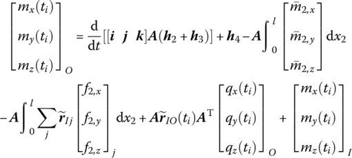
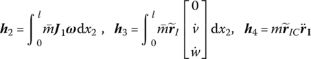
Linearizing h2, h3 and h4, respectively
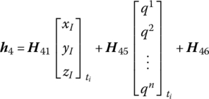
where
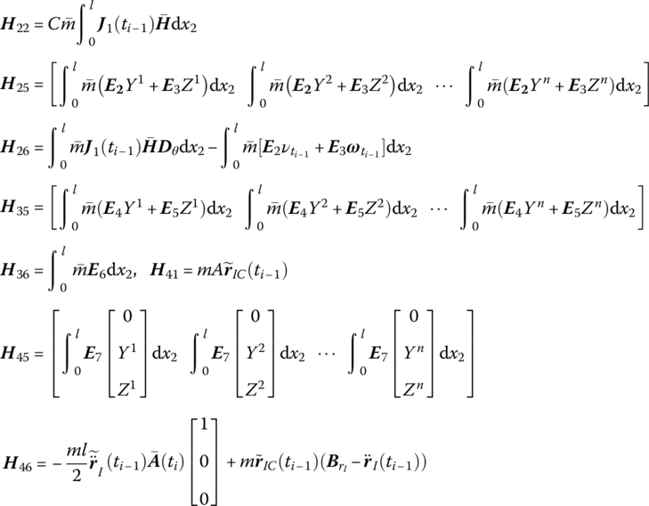
![]() and
and ![]() are determined by Equation (8.62).
are determined by Equation (8.62).
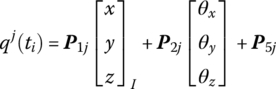
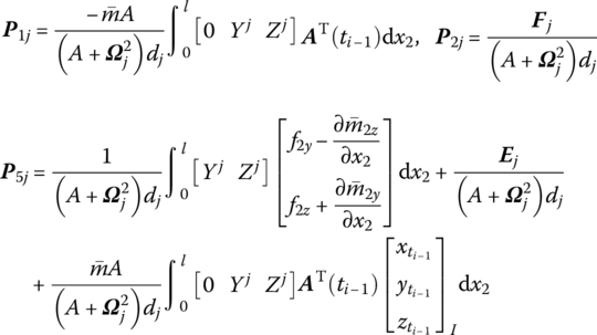
Substituting Equations (8.178) to (8.180) into Equation (8.177) and rearranging yields
where
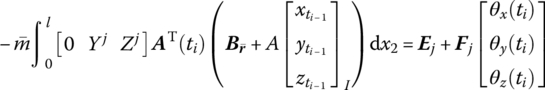
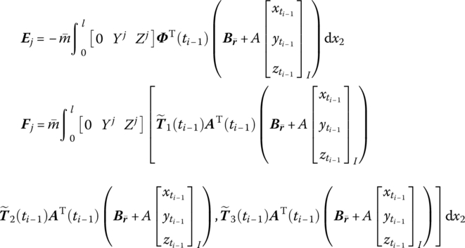
Substituting Equations (8.65) and (8.83) into Equation (8.167) and rearranging gives
where
![]() is determined by Equation (8.84), and T1, T2 and T3 are determined by Equation (8.77).
is determined by Equation (8.84), and T1, T2 and T3 are determined by Equation (8.77).
Since the rotation angles of the beam at the input and output ends are equal in the floating frame, we obtain
The generalized coordinates are the same at an arbitrary point of the beam, which gives
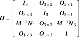
From Equations (8.173), (8.181), (8.182), (8.183) and (8.184), the transfer equation of a Euler–Bernoulli beam with large spatial motion is obtained and denoted as
The transfer matrix is
The state vectors are
8.10 Transfer Matrices of Fixed Hinges Connected to a Beam with Large Spatial Motion
There are three kinds of fixed hinges connected to a beam with spatial motion: (1) the inboard body is rigid and the outboard body is flexible, (2) both the inboard and outboard bodies are flexible, and (3) the inboard body is flexible and the outboard body is rigid.
8.10.1 Transfer Matrix of a Fixed Hinge whose Inboard Body is a Rigid Body and whose Outboard Body is a Beam
For a transverse vibration beam fixed on the rigid body with fundamental motion, the position coordinates, orientation angles, internal forces and internal moments of fixed hinge are equal at its input and output ends. The generalized coordinates describing the deformation of the beam can be determined as follows.
The orthogonality of eigenvector functions in the theory of vibration yields

where Ωk is the kth order natural frequency.
Using the modal analysis method to deal with transverse deformation in transverse vibration beam Equations (8.152) and (8.153), substituting Equations (8.146) and (8.171) into Equations (8.152) and (8.153) and linearizing, we obtain

Multiplying both sides of Equation (8.188) by  and integrating along the axis direction of the beam gives

yielding
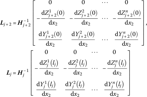
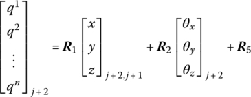
where
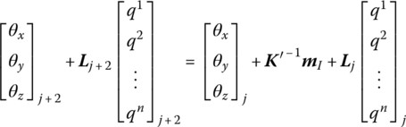
Substituting Equation (8.190) into Equation (8.189) and rearranging yields
where
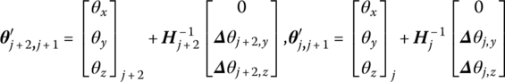
Hence, the transfer equation of a fixed hinge whose inboard body is rigid and whose outboard body is a beam is
The state vectors are

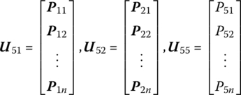
The transfer matrix is
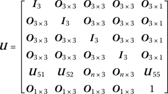
where
8.10.2 Transfer Matrix of a Fixed Hinge whose Inboard and Outboard Bodies are Beams
For a transverse vibration beam fixed on a moving beam, the position coordinates, internal forces and internal moment of the fixed hinge are equal at its input and output ends. The orientation angles and generalized coordinates describing the deformation of outboard beam can be determined as follows.
According to the derivation of the fixed hinge whose inboard body is a rigid body and whose outboard body is a beam in section 8.10.1 and the vibration equations of outboard beam, we obtain

where ![]() is similar to
is similar to ![]() in the transfer matrix of the fixed hinge whose inboard body is rigid and whose outboard body is a beam, and
in the transfer matrix of the fixed hinge whose inboard body is rigid and whose outboard body is a beam, and ![]() are the orientation angles of the body‐fixed coordinate system of the outboard beam, which is determined by the state vector of the output end of the inboard beam.
are the orientation angles of the body‐fixed coordinate system of the outboard beam, which is determined by the state vector of the output end of the inboard beam.
The direction transformation matrices ![]() and
and ![]() have the following relation
have the following relation
where
Yk, Zk, x2, l and qk are parameters of the inboard beam.
Then
where
Substituting Equation (8.196) into Equation (8.194) yields

The transfer equation of the fixed hinge whose inboard and outboard bodies are beams becomes
The state vectors are

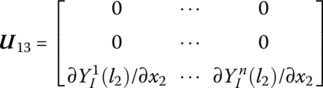
The transfer matrix is
8.10.3 Transfer Matrix of a Fixed Hinge whose Inboard Body is a Beam and whose Outboard Body is a Rigid Body
The derivation of the transfer matrix of a fixed hinge whose inboard body is a Euler–Bernoulli beam and whose outboard body is a rigid body is similar to that in section 8.5. By eliminating rows corresponding to the generalized coordinates in Equation (8.199), the transfer equation of the fixed hinge whose inboard body is a beam and whose outboard body is a rigid body can be obtained:
The state vectors are
The transfer matrix is
where the meaning of all elements is the same as in Equation (8.199).
8.11 Transfer Matrices of Smooth Hinges Connected to a Beam with Large Spatial Motion
There are four kinds of smooth hinges connected to a spatial beam: (1) both the outboard and inboard bodies are rigid bodies, (2) the outboard body is flexible and the inboard body is rigid, (3) both the outboard and inboard bodies are flexible, and (4) the outboard body is rigid and the inboard body is flexible. Here, we introduce two kinds of transfer matrices of smooth hinges connected to a spatial beam: (1) the outboard body is a beam and (2) the outboard body is a rigid body.
8.11.1 Transfer Matrix of a Smooth Hinge whose Inboard Body is a Rigid Body and whose Outboard Body is a Beam
For a smooth hinge, the position coordinates, internal forces and internal moments of its input and output ends are equal. The generalized coordinates which are used to describe the deformation of a Euler–Bernoulli beam and orientation angles of the floating frame are described as follows.
Linearizing the vibration equations of the beam yields
where the meaning of ![]() is similar to that in Equation (8.191).
is similar to that in Equation (8.191).
The moment of connection hinge at the output end of the beam is zero. From the rotational equations of the beam we obtain
where I is the input end of the outboard beam, which is also the output end of the smooth hinge. ![]() ,
, ![]() ,
, ![]() ,
, ![]() and
and ![]() are submatrices of the transfer matrix of the flexible beam.
are submatrices of the transfer matrix of the flexible beam.
As ![]() , this yields
, this yields
As the position coordinates and internal forces at the input and output ends are equal, combining Equations (8.202) and (8.203) gives
where
The transfer equation of a smooth hinge whose inboard body is a rigid body and whose outboard body is a beam becomes
The state vectors are
The transfer matrix is

8.11.2 Transfer Matrix of a Smooth Hinge whose Inboard and Outboard Bodies are Beams
For smooth hinge whose inboard and outboard bodies are Euler–Bernoulli beams, its position coordinates, internal forces and internal moment at the input and output ends are equal. Similar to the smooth hinge whose inboard body is a rigid body and whose outboard body is a beam, the orientation angles of the floating frame and the generalized coordinates of deformation of the outboard beam of a smooth hinge whose inboard and outboard bodies are beams can be obtained from the vibration equation and the rotational equation of the outboard beam. If the internal moment at the output end of the outboard beam is zero, the description is shown in Equations (8.202) and (8.205).
The transfer equation of a smooth hinge whose inboard and outboard bodies are beams yields
The state vectors are
The transfer matrix is
where the meaning of all elements is similar to that in Equation (8.207).
8.11.3 Transfer Matrix of a Smooth Hinge whose Inboard Body is a Beam and whose Outboard Body is a Rigid Body
The derivation of the transfer matrix of a smooth hinge whose inboard body is a beam and whose outboard body is a rigid body is the same as that in section 8.5, except that the rows corresponding to the generalized coordinates in Equation (8.209) are eliminated. Therefore, the transfer equation of a smooth hinge whose inboard body is a beam and whose outboard body is a rigid body yields
The state vectors are
The transfer matrix is
where the meanings of all elements are the same as those in Equation (8.209).
8.12 Transfer Matrices of Spring Hinges Connected to a Beam with Large Spatial Motion
Here, an elastic hinge composed of a massless linear spring and a massless torsional spring, is considered. Let element ![]() denote the spring hinge, and j and
denote the spring hinge, and j and ![]() denote its inboard and outboard bodies, respectively. According to the equilibrium of forces at the input and output ends of the spring, the following equations can be obtained
denote its inboard and outboard bodies, respectively. According to the equilibrium of forces at the input and output ends of the spring, the following equations can be obtained
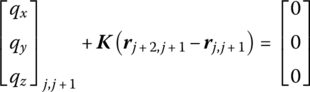
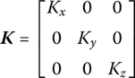
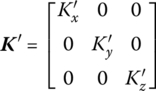
where ![]() is the stiffness coefficient matrix of the spring, and Kx, Ky and Kz are the coefficients of spring stiffness along the three axes of the inertia coordinate system.
is the stiffness coefficient matrix of the spring, and Kx, Ky and Kz are the coefficients of spring stiffness along the three axes of the inertia coordinate system.
Then
For a torsional spring, that is
where ![]() is the stiffness coefficient matrix of the torsional spring, and
is the stiffness coefficient matrix of the torsional spring, and ![]() and
and ![]() are the orientation angles of the torsional spring at the input and output ends, respectively.
are the orientation angles of the torsional spring at the input and output ends, respectively. ![]() are the stiffness coefficients of the torsional spring along the three axes of the inertial coordinate system.
are the stiffness coefficients of the torsional spring along the three axes of the inertial coordinate system.
The derivation of the transfer matrices of spring hinges connected to a Euler–Bernoulli beam with large spatial motion is discussed in three situations in the following sections.
8.12.1 Transfer Matrix of a Spring Hinge whose Inboard and Outboard Bodies are Beams
For a spring hinge whose inboard body j and outboard body ![]() are beams moving in space, the transformation relation between the orientation angles of the inboard beam and the generalized coordinates describing the deformation of the outboard beam can be determined as follows.
are beams moving in space, the transformation relation between the orientation angles of the inboard beam and the generalized coordinates describing the deformation of the outboard beam can be determined as follows.
The transformation matrices ![]() and
and ![]() of the spring hinge at the input end and its inboard beam have the relation
of the spring hinge at the input end and its inboard beam have the relation
where
![]() ,
, ![]() , x2, lj and
, x2, lj and ![]() are interrelated parameters of the inboard beam j.
are interrelated parameters of the inboard beam j.
![]() and
and ![]() are the transformation matrices of the spring hinge at the input end and its outboard beam, respectively. It has the relation
are the transformation matrices of the spring hinge at the input end and its outboard beam, respectively. It has the relation
where
![]() ,
, ![]() , x2 and
, x2 and ![]() are parameters of outboard beam
are parameters of outboard beam ![]() .
.
Linearizing Equations (8.217) and (8.219) yields
where

that is
Substituting Equations (8.217), (8.220) and (8.222) into Equation (8.215), we obtain
where
Similar to Section 8.8.1, linearizing the equations of motion of the outboard beam ![]() , we obtain
, we obtain
where
The meaning of ![]() is similar to Equation (8.191).
is similar to Equation (8.191).
According to Equations (8.214), (8.223) and (8.224), this yields

where the order of ![]() is
is ![]() and the order of
and the order of ![]() is
is ![]() :
:
According to Equations (8.214) and (8.225), the transfer equation of a spring hinge whose inboard and outboard bodies are beams moving in space is
The state vectors are
The transfer matrix is

where ![]() .
.
8.12.2 Transfer Matrix of a Spring Hinge whose Inboard Body is a Rigid Body and whose Outboard Body is a Beam
For a spring hinge whose inboard body is a rigid body and whose outboard body is a beam, the orientation angles ![]() of the spring hinge at the input end are the orientation angles of its inboard rigid body. According to the derivation of the transfer matrix of a spring hinge whose inboard and outboard bodies are beams, the transfer matrix of a spring hinge whose inboard body is a rigid body and whose outboard body is a beam can be obtained by eliminating the columns corresponding to the generalized coordinates of the inboard beam in Equation (8.227). Therefore, the transfer equation of a spring hinge whose inboard body is a rigid body and whose outboard body is a beam is
of the spring hinge at the input end are the orientation angles of its inboard rigid body. According to the derivation of the transfer matrix of a spring hinge whose inboard and outboard bodies are beams, the transfer matrix of a spring hinge whose inboard body is a rigid body and whose outboard body is a beam can be obtained by eliminating the columns corresponding to the generalized coordinates of the inboard beam in Equation (8.227). Therefore, the transfer equation of a spring hinge whose inboard body is a rigid body and whose outboard body is a beam is
The state vectors are

The transfer matrix is

where the meanings of all elements are the same as those in Equation (8.227).
8.12.3 Transfer Matrix of a Spring Hinge whose Inboard Body is a Beam and whose Outboard Body is a Rigid Body
For a spring hinge whose inboard body is a beam and whose outboard body is a rigid body, the orientation angles ![]() of the spring hinge at the output end are exactly the orientation angles of its outboard rigid body. According to the derivation of the transfer matrix of a spring hinge whose inboard and outboard bodies are beams, let
of the spring hinge at the output end are exactly the orientation angles of its outboard rigid body. According to the derivation of the transfer matrix of a spring hinge whose inboard and outboard bodies are beams, let ![]() , so from Equation (8.223) we obtain
, so from Equation (8.223) we obtain
According to Equations (8.214) and (8.223), the transfer equation of a spring hinge whose inboard body is a Euler–Bernoulli beam and whose outboard body is a rigid body is
The state vectors are

The transfer matrix is

where the meanings of ![]() ,
, ![]() and
and ![]() are the same as in Equations (8.227) and (8.223).
are the same as in Equations (8.227) and (8.223).
8.13 Algorithm of the Discrete Time Transfer Matrix Method for Multi‐flexible‐body Systems
The algorithm for the computer solution of MRFS dynamics using the DTTMM for MRFSs can be described as follows:
- Establish a floating coordinate system for each flexible element in the system, determine the numbers of generalized coordinates which describe the deformation of flexible elements, and determine the initial conditions and boundary conditions of the system. Let
 .
. - Compute the linearization coefficients A, Bz or
 , C, Dz or
  , A, Φ, T1, T2, T3,
  ,
,  and so on for each element at time ti by linearization approach, and determine the initial conditions of the generalized coordinates and the system parameters at time ti.
 - Obtain the transfer matrix for each element and the overall transfer matrix of the system at time ti.
- Apply the boundary conditions and the overall transfer matrix to compute the unknown quantities of the boundary state vectors at time ti.
- Obtain the state vectors of all elements at time ti by computing the transfer equations of each element successively.
- Use the state vectors at time ti to compute the position coordinates, the rotation angle and the generalized coordinates which describe the deformation of the flexible elements, then solve their first‐order and second‐order derivatives with respect to time.
- Use the modal analysis method to solve the deformation of the flexible element at the investigated positions.
- Let
 , use the computational results of the last step as the initial conditions and repeat all the above steps from step (2) until the time required for complete analysis.
8.14 Planar Multi‐flexible‐body System Dynamics

Figure 8.6 Three‐pendulum model of a multi‐rigid‐flexible system.
Figure 8.7 Time history of the dynamics of three pendulums moving in a plane: (a) orientation angle of rigid body 2, (b) orientation angle of the floating frame, (c) orientation angle of rigid body 6 and (d) deformation in the mid‐point of the beam.
Figure 8.8 Dynamics model of a rigid‐flexible four‐bar linkage.
Figure 8.9 Time history of the dynamics of a rigid‐flexible four‐bar linkage moving in a plane: (a) orientation angle of rigid body 5, (b) orientation angle of beam 4 and (c) deformation in the mid‐point of the beam 4.
8.15 Spatial Multi‐flexible‐body System Dynamics
Figure 8.10 Model of a rigid‐flexible‐body system composed of three pendulums moving in space.
Figure 8.11 Time history of the dynamics of three pendulums moving in space: (a) deformation in the mid‐point of beam 4, (b) deformation of beam 4 in z2, (c) angle of rigid body 2, (d) angle of floating frame of beam 4 and (e) angle of rigid body 6.