
5
Transfer Matrix Method for Multi‐rigid‐body Systems
5.1 Introduction
Multibody system dynamics methods (MSDMs) have developed rapidly in the last 50 years and provide powerful tools for studying the dynamics of various mechanical systems. Although the various classical MSDMs have different styles, at the same time almost all of them share the following characteristics: first, it is necessary to develop the global dynamics equations of the system, and they have to be deduced again if the system’s topological structure is changed; second, the order of the global dynamics equations is not less than the number of degrees of freedom of the system, which may become very high for complex systems resulting in a rather long computational time.
The approach proposed in this chapter is different from the above and has a different origin. In 1986, Kumar and Sankar developed a discrete time transfer matrix method (DTTMM) for the structural dynamics of time‐variant systems by combining the transfer matrix method with a numerical integration procedure. In 1989, Rui and others extended the transfer matrix method to multibody systems (MSTMM) for vibration analysis of linear multi‐rigid‐flexible‐body systems by developing new transfer matrices, where eigenvalues of linear multi‐rigid‐flexible‐body systems can be computed easily and with high precision. For general nonlinear multi‐rigid‐body and multi‐rigid‐flexible‐body systems, the discrete time transfer matrix method of multibody systems (MSDTTMM) was developed by combining the MSTMM with a numerical integration procedure.
To improve computational precision and simplify the transfer matrices of the MSTMM, a novel MSTMM is presented in this chapter. The translational and angular accelerations together with internal forces and moments are taken as new state variables instead of position coordinates in the original MSTMM. This results in totally different transfer matrices of elements and algorithms compared with the original MSTMM. The proposed method expands the advantages of the MSTMM by allowing more sophisticated numerical integration procedures such as the Runge–Kutta method to be used: no global dynamics equations of the system are required, matrices have low order, setup of global transfer equation is highly programmable and solution allows high computational precision since linearization is not required anymore. The new method is simple, straightforward, efficient, practical and provides a powerful tool for multibody system dynamics (MSD).
5.2 State Vectors, Transfer Equations and Transfer Matrices
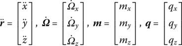
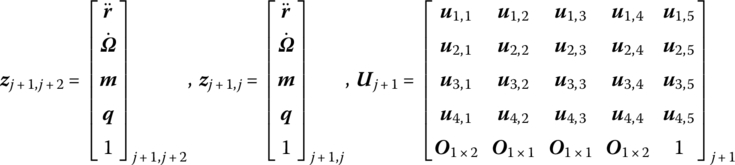
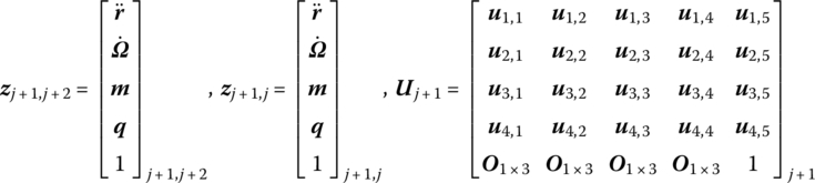
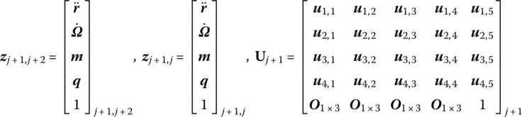
For simplicity, a chain multibody system is taken as an example in the following. The new state vectors of the input ends and output ends of any rigid bodies and hinges moving in space are defined as
or
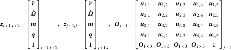
where
![]() , ÿ,
, ÿ, ![]() ,
, ![]() ,
, ![]() and
and ![]() are the absolute accelerations of the connection end with respect to the inertial reference system oxyz and the corresponding absolute angular accelerations in the directions of x, y and z, mx, my, mz, qx, qy and qz are the corresponding internal torques and internal forces in the same reference system, respectively, and
are the absolute accelerations of the connection end with respect to the inertial reference system oxyz and the corresponding absolute angular accelerations in the directions of x, y and z, mx, my, mz, qx, qy and qz are the corresponding internal torques and internal forces in the same reference system, respectively, and ![]() ,
, ![]() , m and q are the column vectors of absolute accelerations, absolute angular accelerations, internal torques and internal forces in oxyz, respectively.
, m and q are the column vectors of absolute accelerations, absolute angular accelerations, internal torques and internal forces in oxyz, respectively.
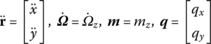
For a chain system moving in a plane, the state vectors of the input ends and output ends of any rigid bodies and hinges are defined as
or
where
Then the dynamics equations of the jth element can be assembled into a single transfer equation
The transfer equation describes the transfer relationship between the state vectors at two ends of the jth element and has a similar form to but total different contents from a general transfer equation used in the original MSTMM. Here, the matrix Uj(ti) is the transfer matrix of the jth element which is known at time instant ti. Its order is always (13 × 13) for any dynamics of a chain multi‐rigid‐body system moving in space or (7 × 7) for any dynamics of a chain multi‐rigid‐body system moving in a plane.
5.3 Overall Transfer Equation and Overall Transfer Matrix
According to Newton’s third law, the state vector of the output end of an inboard element is equal to the state vector of the input end of an outboard element for any two adjoining elements in a multibody system. So, the overall transfer equation and transfer matrix of the system, which relates the state vectors at boundaries of the system, can be assembled for any chain multibody system as follows:
It can be seen clearly from the overall transfer equation that the order of the overall transfer matrix of the system is equal to the order of the transfer matrix of an element for a chain system, and it does not increase even if the degrees of freedom of the system increase. Irrespective of the size of a multibody system, the highest order of the overall transfer matrix is the same as the order of the transfer matrix of a single body, that is, (13 × 13) for the dynamics of a chain multi‐rigid‐body system moving in space or (7 × 7) for the dynamics of a chain multi‐rigid‐body system moving in a plane. The matrices involved in the new MSTMM are therefore always small, which greatly reduces the computational time and the memory storage requirement.
5.4 Transfer Matrix of a Planar Rigid Body
A planar rigid body with a single input end and a single output end is shown in Figure 5.1, where points I, O and C denote the inboard end, outboard end and mass center of the rigid body, respectively. The subscript 2 denotes the body‐fixed coordinate system whose origin O2 coincides with the inboard end I of the rigid body, while oxyz is the inertial coordinate system. The structural parameters of the rigid body are represented in a body‐fixed coordinate system.

Figure 5.1 Planar rigid body.
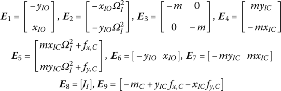
Geometrical equations can be obtained
where rK and rI are the global position vectors, decomposed in the inertial coordinate system, of point K and the input end I, respectively. The same formula also applies for the output end O and the mass center C. rIK is the position vector of point K with respect to the input end I, decomposed in the inertial coordinate system.
Using the Newton–Euler method, the dynamics equations of the rigid body can be deduced
where m and ![]() are the mass and the column vector of the absolute acceleration of the mass center, respectively,
are the mass and the column vector of the absolute acceleration of the mass center, respectively, ![]() and
and ![]() are the column vectors of internal forces acting on points I and O,
are the column vectors of internal forces acting on points I and O, ![]() and
and ![]() are the column vectors of external force and the external torque acting on the mass center of the rigid body, JI is the moment of inertia with respect to point I,
are the column vectors of external force and the external torque acting on the mass center of the rigid body, JI is the moment of inertia with respect to point I, ![]() and
and ![]() are the column vectors of internal torques acting on the points I and O,
are the column vectors of internal torques acting on the points I and O, ![]() and
and ![]() are the column vectors of position vectors from I to O and to C, respectively, and
are the column vectors of position vectors from I to O and to C, respectively, and ![]() and ÿI are the components of the column vector of the absolute acceleration of point I, which can be denoted compactly as
and ÿI are the components of the column vector of the absolute acceleration of point I, which can be denoted compactly as ![]() .
.
The rotation of any point of the same rigid body is uniform and can be expressed as
Equations (5.10) to (5.12) can be rewritten as
where
Combining Equations (5.13) to (5.16), the transfer equation and transfer matrix of a rigid body moving in a plane can be obtained

where zO and zI are the state vectors of the inboard end I and outboard end O on the rigid body defined in Equation (5.4), and the order of the transfer matrix of the rigid body moving in a plane is (7 × 7).
5.5 Transfer Matrix of a Spatial Rigid Body
A spatial rigid body with a single input end and a single output end is shown in Figure 5.2, where points I, O and C denote the inboard end, outboard end and mass center of the rigid body, respectively. The subscript 2 denotes the body‐fixed coordinate system whose origin O2 coincides with the inboard end I of the rigid body, while oxyz is the inertial coordinate system. The structural parameters of the rigid body are represented in a body‐fixed coordinate system.
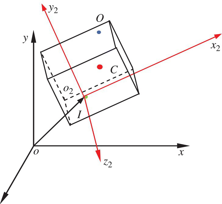
Figure 5.2 Spatial rigid body.
Geometrical equations can be obtained
where rK and lIK are the column vectors of the position coordinate of point K with respect to the inertial coordinate system and the body‐fixed coordinate system, respectively. The same formula applies for points O and C. AI is direction cosine matrix of input end I with respect to the global reference system.
Using the Newton–Euler method, the dynamics equations of the rigid body can be deduced
where m and ![]() are the mass and the column vector of mass center absolute acceleration of the rigid body, qI and qO are the column vectors of internal forces acting on points I and O, fC and mC are the column vectors of external force and the external torque acting on the mass center of the rigid body, GI is the column vector of moment of momentum with respect to point I, mI and mO are the column vectors of internal torques acted on points I and O, rIO and rIC are the column vectors of position vectors from I to O and to C, respectively, and
are the mass and the column vector of mass center absolute acceleration of the rigid body, qI and qO are the column vectors of internal forces acting on points I and O, fC and mC are the column vectors of external force and the external torque acting on the mass center of the rigid body, GI is the column vector of moment of momentum with respect to point I, mI and mO are the column vectors of internal torques acted on points I and O, rIO and rIC are the column vectors of position vectors from I to O and to C, respectively, and ![]() is the column vector of the absolute acceleration of point I.
is the column vector of the absolute acceleration of point I.
The rotation of any point of the same rigid body is uniform and can be expressed as
Equations (5.19) to (5.21) can be rewritten as
where

Combining Equations (5.22) to (5.25), the transfer equation and the transfer matrix of a rigid body moving in space can be obtained
where zO and zI are the state vector of the inboard end I and outboard end O on the rigid body defined in Equation (5.1), and the order of the transfer matrix of the rigid body moving in space is (13 × 13).
5.6 Transfer Matrix of a Planar Hinge
For a smooth pin hinge j, whose inboard body ![]() and outboard body
and outboard body ![]() are moving in a plane, its mass and size are neglected. The position coordinates of its two ends, as well as the corresponding time derivatives, are equal. Newton’s third law of motion says that internal forces acting on its two ends are equal in magnitude but opposite in directions. The “smooth” here means that the internal torques are equal to zeros. Thus the following four groups of equations are obtained.
are moving in a plane, its mass and size are neglected. The position coordinates of its two ends, as well as the corresponding time derivatives, are equal. Newton’s third law of motion says that internal forces acting on its two ends are equal in magnitude but opposite in directions. The “smooth” here means that the internal torques are equal to zeros. Thus the following four groups of equations are obtained.
For a smooth pin hinge j whose outboard body’s outboard hinge is also a smooth pin hinge
The transfer equation for an outboard rigid body of a smooth pin hinge j is
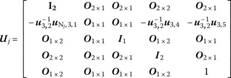
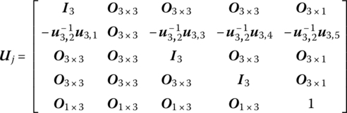
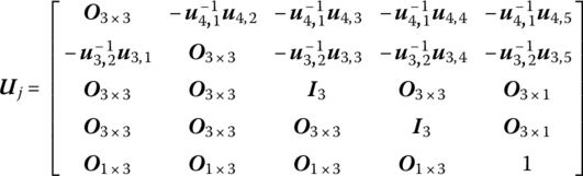
The state vectors and transfer matrix in the form of a partitioned matrix are
The relation of internal moments between the input and output ends of a rigid body is
where um,n is the corresponding partitioned submatrix of ![]() , the transfer matrix of the outboard body, given in Equation (5.34).
, the transfer matrix of the outboard body, given in Equation (5.34).
Substituting the above equations into Equation (5.32), the relation of angular accelerations between the input and output ends of the hinge can be obtained
Combining Equations (5.28) to (5.30) and (5.36) the transfer equation and the transfer matrix of a smooth pin hinge j moving in a plane can be obtained
5.7 Transfer Matrix of a Spatial Hinge
5.7.1 Transfer Equation of a Smooth Ball‐and‐socket Hinge
Similarly, for a smooth ball‐and‐socket hinge j, whose inboard body ![]() and outboard body
and outboard body ![]() are moving in space, its mass and size are also neglected. The position coordinates of its two ends, as well as the corresponding time derivatives, are equal. The internal torques are equal to zeros. Thus the following four groups of equations are obtained.
are moving in space, its mass and size are also neglected. The position coordinates of its two ends, as well as the corresponding time derivatives, are equal. The internal torques are equal to zeros. Thus the following four groups of equations are obtained.
For a smooth ball‐and‐socket hinge j whose outboard body’s outboard hinge is also a smooth ball‐and‐socket hinge
The transfer equation for an outboard rigid body of a smooth ball‐and‐socket hinge j is
The state vectors and transfer matrix in the form of a partitioned matrix are
The relation of internal moments between the input and output ends of a rigid body is
where um,n is the corresponding partitioned submatrix of ![]() , the transfer matrix of the outboard body, given in Equation (5.45).
, the transfer matrix of the outboard body, given in Equation (5.45).
Substituting the above equations into Equation (5.43), the relation of angular accelerations between the input and output ends of the hinge can be obtained
Combining Equations (5.39) to (5.41) and (5.47), the transfer equation and transfer matrix of a smooth ball‐and‐socket hinge j can be obtained
5.7.2 Transfer Equation of a Smooth Pin Hinge Moving in Space
A smooth pin hinge j whose inboard rigid body is ![]() and outboard rigid body is
and outboard rigid body is ![]() is shown in Figure 5.3. The position coordinates, as well as the corresponding time derivatives, and internal forces are equal, and the internal torque is equal to zero along the relative‐rotation axis. If the relative rotation angle of the smooth pin hinge j is denoted by Θj, then there are the following five groups of equations
is shown in Figure 5.3. The position coordinates, as well as the corresponding time derivatives, and internal forces are equal, and the internal torque is equal to zero along the relative‐rotation axis. If the relative rotation angle of the smooth pin hinge j is denoted by Θj, then there are the following five groups of equations
where
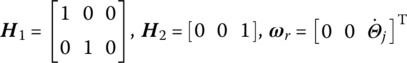
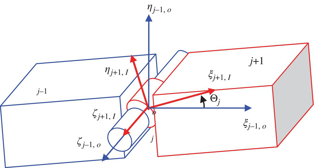
Figure 5.3 Smooth pin hinge moving in space.
![]() is the direction cosine matrix of the input‐end body‐fixed coordinate system of body element
is the direction cosine matrix of the input‐end body‐fixed coordinate system of body element ![]() .
.
For a smooth pin hinge j whose outboard body’s outboard hinge is also a pin hinge
where ![]() is the direction cosine matrix of the output‐end body‐fixed coordinate system of body element
is the direction cosine matrix of the output‐end body‐fixed coordinate system of body element ![]() .
.
The transfer equation for an outboard rigid body ![]() of the smooth pin hinge j is
of the smooth pin hinge j is
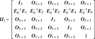
The state vectors and transfer matrix in the form of a partitioned matrix are
The relation of internal moments between the input and output ends of a rigid body ![]() is
is
where um,n is the corresponding partitioned submatrix of ![]() ,the transfer matrix of the outboard body, given in Equation (5.57).
,the transfer matrix of the outboard body, given in Equation (5.57).
Substituting the above equations into Equation (5.52), the relation of angular accelerations between the input and output ends of a smooth pin hinge j can be obtained
where
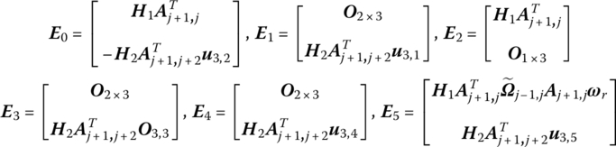
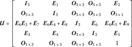
Combining Equations (5.50), (5.51), (5.53) and (5.59) and adjusting their sequences according to the configuration of the state vector, the transfer equation and transfer matrix of the smooth pin hinge j can be obtained
5.8 Transfer Matrix of an Acceleration Hinge
An acceleration hinge is a totally new concept that can be considered to be a fictitious hinge presented in the new MSTMM. The acceleration hinge describes the elastic internal forces, elastic internal torques, damping internal forces and damping internal torques due to the relative deformation of the hinge.
The acceleration and angular acceleration of the output end of an acceleration hinge can be obtained from the transfer matrix of its outboard bodies. The processes to deduce the transfer matrix are similar for a smooth hinge and an acceleration hinge.
The internal forces and torques of the elastic hinge are treated as torques acting on its inboard and outboard bodies, respectively.
As stated previously, once the action and reaction forces of an elastic hinge are treated as part of the external forces acting on the connected body elements, the elastic hinge can be dealt with as an acceleration hinge.
For an acceleration hinge j moving in space, whose inboard body ![]() and outboard body
and outboard body ![]() are all rigid bodies moving in space, the internal forces and torques are zeros at its two ends. Thus the following four groups of equations can be obtained:
are all rigid bodies moving in space, the internal forces and torques are zeros at its two ends. Thus the following four groups of equations can be obtained:
For an acceleration hinge j whose outboard body’s outboard hinge is also an acceleration hinge
The transfer equation for the outboard rigid body of the acceleration hinge j is
The state vectors and transfer matrix in the form of a partitioned matrix are
The relation of internal moments between the input and output ends of a rigid body is
where um,n is the corresponding partitioned submatrix of ![]() , the transfer matrix of the outboard body, given in Equation (5.69).
, the transfer matrix of the outboard body, given in Equation (5.69).
Substituting the above equations into Equation (5.67), the relation of angular accelerations between the input and output ends of the hinge can be obtained
In the same way, we can obtain
Combining Equations (5.62), (5.64), (5.71) and (5.72), the transfer equation and transfer matrix of acceleration hinge j can be obtained
It can be proved and understood easily that the transfer equation and transfer matrix of an acceleration hinge moving in a plane are similar, corresponding to Equations (5.73) and (5.74), respectively, moving in space.
5.9 Algorithm of the Transfer Matrix Method for Multibody Systems
The algorithms of the new MSTMM and the original MSTMM are different because of the different state vectors defined in the two situations. Following the formulations given above, the motion quantities of a multibody system at different time instants for different subsystems can be obtained as follows:
- Decide the initial conditions and system properties of the multibody system.
- Set i = 1.
- Knowing the initial conditions
 ,
,  ,
,  ,
,  , etc. and the system properties at time
  , formulate the transfer matrix for each subsystem and the overall transfer matrix.
 - Apply boundary conditions to the end state vectors of the system and calculate the unknown quantities in the boundary state vectors as a function of the elements of the overall transfer matrix.
- Knowing all the elements in the boundary state vector, the state vectors of each subsystem at time instant
 can be computed by successive multiplication of the transfer matrices using the transfer equation of the elements.
 - By using the initial conditions
 ,
,  ,
,  and
and  , and the computed values of the accelerations
  and angular accelerations
  at
at  , compute the values of position coordinates r(ti), velocities
  , orientation angles θ(ti) and
  , etc. at time ti using any numerical integration procedures, for example the Runge–Kutta method.
 - Let
 , use the computed values of the last step as the initial conditions, and return to step 3. This procedure is repeated until the final time step is achieved.
5.10 Numerical Examples of Multibody System Dynamics
To verify the new MSTMM, the dynamics of a pendulum system consisting of three rigid body moving in space and the dynamics of space mechanical arm system are numerically calculated by the proposed method and the Newton–Euler method, respectively.
5.10.1 Dynamics of a Spatial Multibody System with Ball‐and‐socket Hinges
A spatial three pendulum system with three rigid bodies moving in space and connected by three smooth ball‐and‐socket hinges under the effect of gravity is shown in Figure 5.4. The body elements and the hinge elements are numbered: 0, 2 and 4 denote the sequence numbers of the smooth ball‐and‐socket hinges, and 1, 3 and 5 denote the sequence numbers of the body elements. The structure parameters of the three rigid bodies are the same. The coordinates of the mass center and the output point, the moment of inertia relative to the input‐end body‐fixed coordinate system, are
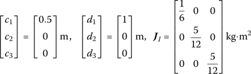
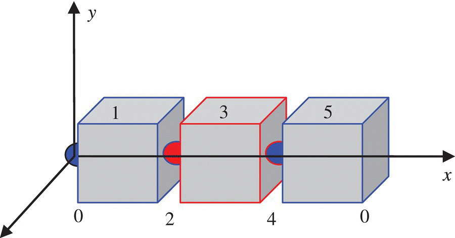
Figure 5.4 Dynamics model of a spatial three‐pendulum system.
The initial conditions of the system are

where ![]() represents the space three angles (
represents the space three angles (![]() ) of body element j.
) of body element j.
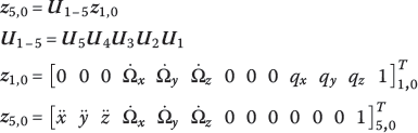
The overall transfer equation and the overall transfer matrix and boundary conditions of the system are
The time histories of the space three angles of rigid body 1 of the system obtained by the proposed method and by the Newton–Euler method are shown in Figure 5.5, represented with ‘line’ and ‘×’ respectively. It can be seen clearly from Figure 5.5 that the computational results of the two methods are in good agreement.
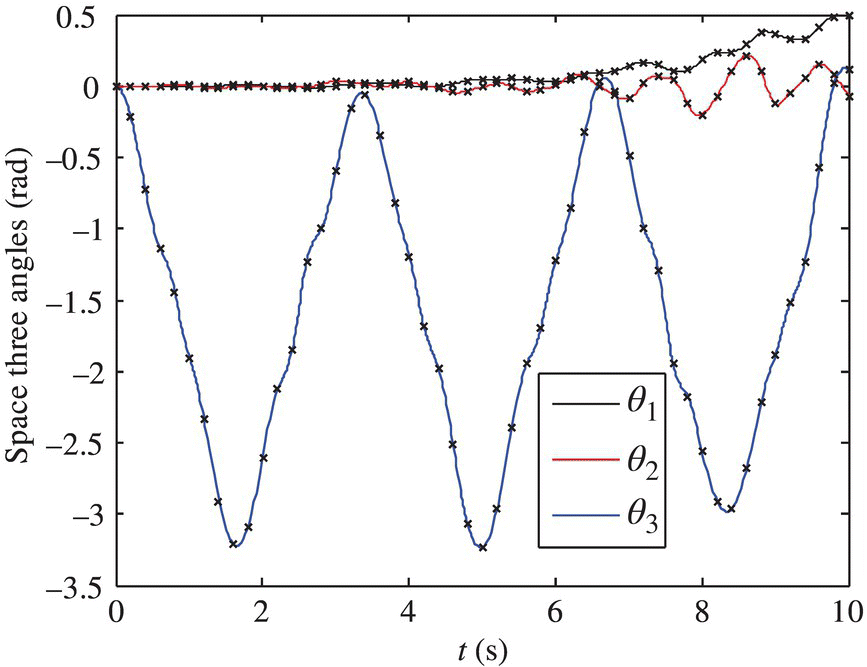
Figure 5.5 Time history of the space three angles of body element 1.
5.10.2 Dynamics of a Spatial Multibody System with Pin Hinges
A spatial mechanical arm system with three rigid bodies moving in space and connected by three smooth pin hinges under the effect of gravity is shown in Figure 5.6. The body elements and the hinge elements are numbered uniformly: 0, 2 and 4 denote the sequence numbers of the smooth pin elements, and 1, 3 and 5 denote the sequence numbers of the body elements. The structure parameters of the three rigid bodies are the same. The coordinates of the mass center and the output point, the moment of inertia relative to the input‐end body‐fixed coordinate system, are
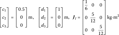
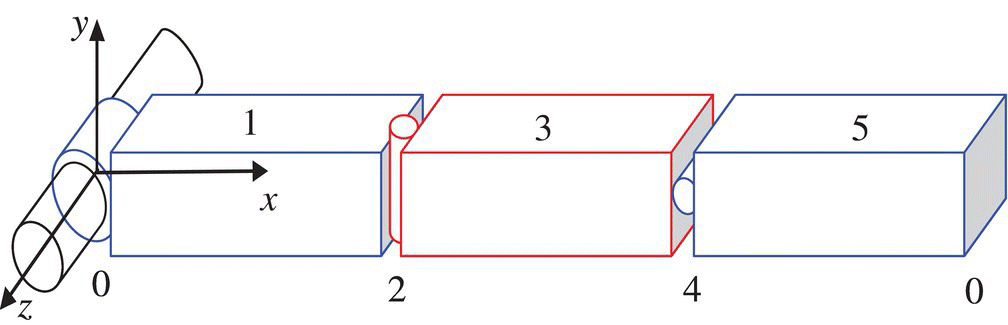
Figure 5.6 Spatial 3 degrees of freedom arm.
The relative rotation angle of pin element j is Θj and the initial conditions of the system are
The overall transfer equation and the overall transfer matrix and boundary conditions of the system are

The time histories of the relative rotation angles of the three pin hinges of the system obtained by the proposed method and by the Newton–Euler method are shown in Figure 5.7, represented with ‘line’ and ‘×’ respectively. It can be seen clearly from Figure 5.7 that the computational results of the two methods are in good agreement.
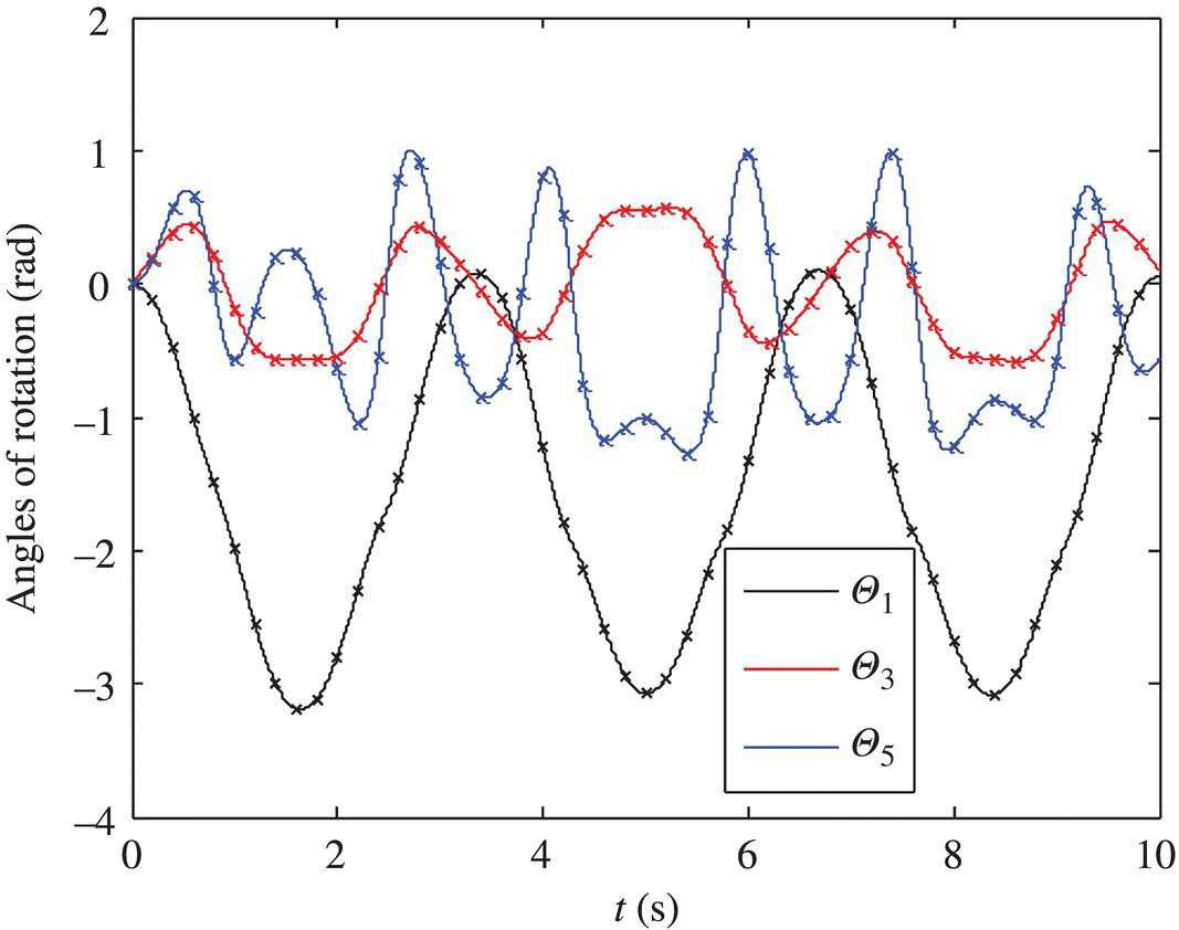
Figure 5.7 Time history of the relative rotation angles of the three pin hinges.
5.10.3 Dynamics of a Spatial Multibody System with Spring and Damping Hinges
Here we choose a multibody system the same as the one given in section 5.10.2 to illustrate the use of spring and damping hinges moving in space. The only difference between the dynamic model in this section and that in section 5.10.2 is that the original smooth pin hinges are substituted by corresponding spring and damping hinges. The corresponding coefficients of the springs and dampers are appropriately selected according to the dynamical parameters of the system. One appropriate group of coefficients is
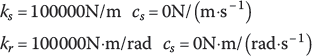
where ks and cs are the coefficients of the springs and dampers, and kr and cr are the coefficients of the rotary springs and dampers, which are used to simulate the connection relationship of the original smooth pin hinges.
The time histories of the relative rotation angles of the three hinges obtained by the smooth pin hinge model and by the elastic and damping hinges model are shown in Figure 5.8, represented with ‘line’ and ‘×’ respectively. It can be seen clearly from Figure 5.8 that the computational results of the two models are in good agreement.
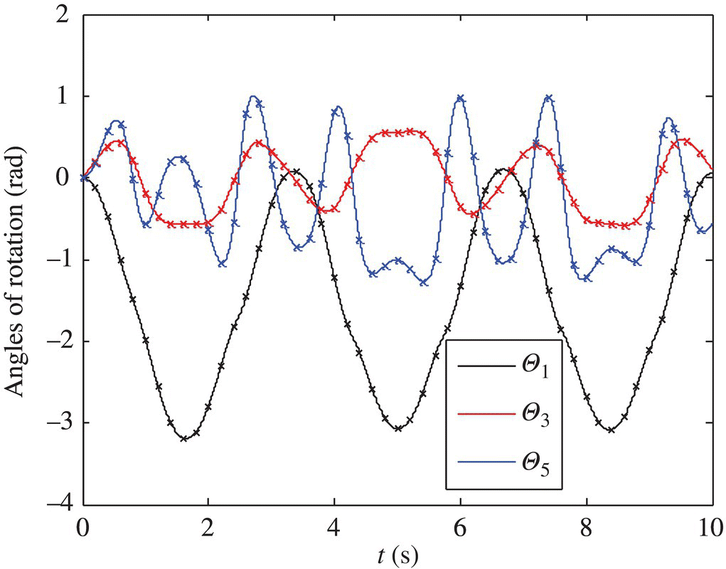
Figure 5.8 Time history of the relative rotation angles of the three hinges.