
11
Theorem to Deduce the Overall Transfer Equation Automatically
11.1 Introduction
The transfer matrix method for multibody systems (MSTMM) provides a new idea, a simple and efficient method of studying complex multibody system dynamics (MSD) that differs from all previous ways. The MSTMM can be applied widely to the dynamics of complex multibody systems with various topologies, such as chain multibody systems, tree multibody systems, closed‐loop multibody systems, general multibody systems etc. In principle, as long as the transfer matrix of the element is obtained, various MSD problems could be solved with ease. Applying the MSTMM, according to the topology figure of the system dynamics model and the automatic deduction theorem of the overall transfer equation, with the transfer matrix of each element in a system the overall transfer equation and overall transfer matrix of the system would be deduced manually or by computer. Then with the substitution of the system boundary condition into the overall transfer equation of the system, the overall transfer equation of the system and the transfer equation of the element can be solved.
For general MSD methods, the global dynamics equation of the system should be established again if there is any change in the elements. However, the same kinds of elements (elements with the same input end number and motion mode) share the same transfer matrix in various multibody systems. Therefore, the same transfer matrix expression can be used without making any changes once the transfer matrix of one element has been deduced. Such an important characteristic of the element transfer matrix makes the transfer matrix method of MSD easy to learn and convenient to use. In addition, after the increase or decrease in elements, the overall transfer equation of the new system can be obtained by adding (multiplying) or deleting the element transfer matrix at a corresponding position and there is no need for re‐deduction.
11.2 Topology Figure of Multibody Systems
Any complex MSD model is composed of various body elements and hinge elements. To make a clear and intuitive description of the transfer relationship and transfer direction between the state vectors of every element in the MSD model, new concepts concerning the topology figure of the MSTMM dynamics model are proposed. The topology figure of the dynamics model of multibody systems is a new graphic representation for the state vector relationship, sequence number of position, sequence number of boundary and transfer direction between body elements and hinge elements, and a concise means for MSD study. The given instruction uses the tree MSD model topology figure shown in Figure 11.1 as an example. The dynamics model topology figure intuitively describes the transfer relationship and transfer direction of the state vector of each element, which is very important for the automatic deduction of the overall transfer equation of a multibody system by handwriting or by computer.
Figure 11.1 Topology figure of a dynamics model of a tree multibody system.
Besides the sign conventions introduced in Chapter 1, the following sign conventions are used in the topology figures:
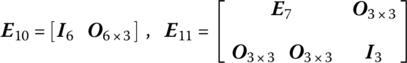
- A circle ○ denotes a body element and the number inside this circle is the sequence number of the body element.
- An arrow → denotes a hinge element and the transfer direction of state vectors, and the number beside the arrow is the sequence number of the hinge element.
- If a body has more than two connection ends with other elements, then one of the connection ends will be regarded as the output end of this body and the other connection ends will be considered as the input ends. As a special case, if a body has only two connection ends, then it will be treated as a single‐input‐single‐output body.
- For a nonboundary end, the subscripts i and j (
 ) in the state vector zi,j of the end denote the sequence numbers of the adjacent body element and hinge element, respectively. For a boundary end, the second subscript j in the state vector zi,j will be replaced by 0, namely we replace zi,j by zi,0. In other words, the second subscript 0 denotes a boundary end and the first subscript i in the state vector zi,0 of the boundary end is the sequence number of the element involved.
 - In a multibody system, only one boundary end is considered as the root, and the state vector of the root is noted as zi,0, where i is the sequence number of the root element, while all the other boundary ends are considered as the tips, and the state vectors of the tips are denoted as zj,0, where j is the sequence number of the tip element. The transfer directions of a system are always from its tips to the root.
- The subscript i in transfer matrix Ui denotes the sequence number of element i. The subscript (i–k) in the transfer matrix
 and the partitioned matrix
  means from element i to element k.
  and
and  mean the successive multiplication of the transfer matrices of all elements in the transfer path from the element i to element k of the system.
11.3 Automatic Deduction of the Overall Transfer Equation of a Closed‐loop System
For the topology figure of the dynamics model of an arbitrary closed‐loop multibody system composed of n elements (including body elements and hinge elements), after “cutting” at the junction of body element n and hinge element 1, the original closed‐loop system becomes a chain system, as shown in Figure 11.3. Setting the two cutting points generated by cutting as the boundary ends of state vectors z1,0 and zn,0, then the original closed‐loop system in Figure 11.2 is transformed into the chain system with equal state vectors z1,0 and zn,0.
Figure 11.2 Topology figure of a closed‐loop system.

Figure 11.3 Topology figure of closed‐loop system after cutting hinge n.
Hence, the transfer equation of a closed‐loop system can be treated as a chain system. It can be automatically deduced that
where
Note that the state vectors of the cutting points are equal, that is
therefore the overall transfer matrix of a chain system can be deduced automatically by handwriting or by computer
where
11.4 Automatic Deduction of the Overall Transfer Equation of a Tree System
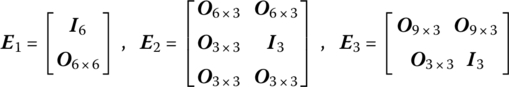
For a body element with more than two endpoints, one endpoint is regarded as the output end while the others are considered as input ends. The transfer equation ought to contain the geometric relation between the first input end and the output end and the dynamics equations governing the motion of the element. It can be proved that the transfer equation of the rigid body j with L input ends can be written as
where subscript j is the sequence number of the body element, O represents the output end, while I1, I2, ![]() , and IL denote the first, the second,…, and the Lth input ends, respectively, zj,O and
, and IL denote the first, the second,…, and the Lth input ends, respectively, zj,O and ![]() are the state vector of output end and the k th input end of the body element, respectively, Uj is the transfer matrix of element j with only one input end and one output end, and
are the state vector of output end and the k th input end of the body element, respectively, Uj is the transfer matrix of element j with only one input end and one output end, and ![]() is the matrix to extract internal force and internal moment from
is the matrix to extract internal force and internal moment from ![]() , called the force extraction matrix.
, called the force extraction matrix.
It can be proved that for the geometric relation between the first input end I1 and the k th output end Ik of the element with L input ends and one output end, the geometric equation is
where Hj is the constant matrix to extract the position coordinates and rotation angles from state vector ![]() , called the position extraction matrix in this book.
, called the position extraction matrix in this book. ![]() is associated with the relative position of the first input end and the k th input end of body j, called the position incidence matrix in this book.
is associated with the relative position of the first input end and the k th input end of body j, called the position incidence matrix in this book.
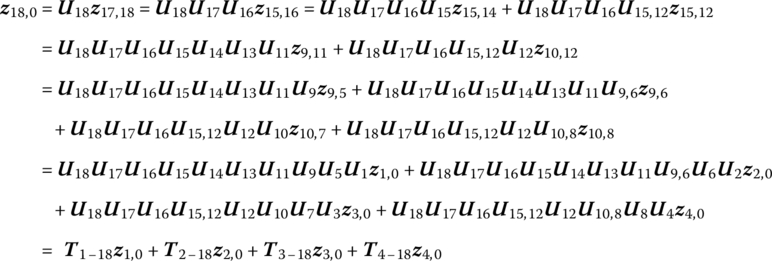
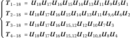
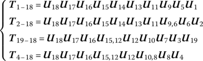
According to the transfer equation and geometric equation of the element, the automatic deduction of the system overall transfer equation can easily be obtained. For the topology figure of the system dynamics model shown in Figure 11.1, joint points P9,5, P10,7, P15,14 and P9,6, P10,8, P15,12 are the first and second input ends of body elements 9, 10 and 15, respectively. According to Equation (11.6), the relation between the state vectors and transfer equations of each element are depicted in Figure 11.4.
Figure 11.4 A system topology structure described by state vectors and transfer equations.
The equation describing the relations among the state vectors of each boundary end shown in Figure 11.4 can be easily deduced, and is known as the system overall transfer equation.
where
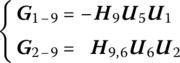
According to Equation (11.7), the geometric equation of body element 9 is
where H9 and H9,6 are the position extraction matrix and position incidence matrix of rigid body 9.
Applying the system topology structure described by state vectors and transfer equations shown in Figure 11.4, the state vectors z9,5 and z9,6 are written as
Substituting Equations (11.11) and (11.12) into Equation (11.10), we obtain
Equation (11.13) can be written as
where
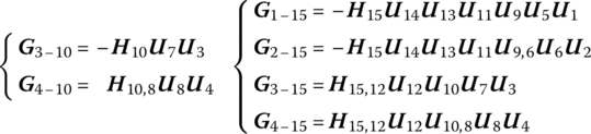
In the same manner, the geometric equations of body elements 10 and 15 can be deduced
where
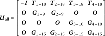
After combining the main transfer equation and the geometric equations of all relevant elements in Equations (11.8), (11.14), (11.16) and (11.17), the overall transfer equation of the system can be obtained:
where
We can rewrite Equations (11.20) and (11.21) as
where

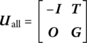
The overall transfer Equation (11.19) of the tree system includes the main transfer Equation (11.8) and geometric Equations (11.14), (11.16) and (11.17), where I is the identity matrix, and the coefficient matrices of all the state vectors in the first column are zero matrices, with the exception of the first row of the overall transfer matrix. In this book, the state vector zall (see Equation (11.20)) is defined as the state vector of the system boundary, while the coefficient matrix Uall (see Equations (11.21) or (11.23)) is defined as the overall transfer matrix of system. The coefficient matrix T (see Equation (11.26)) is defined as main transfer equation coefficient matrix, and the coefficient matrix G (see Equation (11.27)) is defined as the geometric equation coefficient matrix.
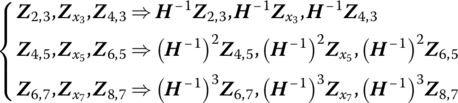
From Equation (11.9), the coefficient matrix of the system boundary state vector of the tree system main transfer equation corresponds to the first row in the overall transfer matrix (see Equation (11.23)), the coefficient matrix of the root state vector is a minus identity matrix and the structure of coefficient matrix T of the branch state vector has the following regular pattern: the transfer matrix (like ![]() and
and ![]() ) from the branch, through the first input end of the multiple input element, to root is equal to the successive multiplication of transfer matrices of all elements along this route, in which the transfer matrix of the involved element with multiple input ends is the transfer matrix of the element with one input (the first input end) and one output (output end). The transfer matrix (
) from the branch, through the first input end of the multiple input element, to root is equal to the successive multiplication of transfer matrices of all elements along this route, in which the transfer matrix of the involved element with multiple input ends is the transfer matrix of the element with one input (the first input end) and one output (output end). The transfer matrix (![]() and
and ![]() ) is equal to the successive multiplication of transfer matrices of all elements, in which the related transfer matrix of the element with multiple input ends is the force extraction matrix of the corresponding input end of the element.
) is equal to the successive multiplication of transfer matrices of all elements, in which the related transfer matrix of the element with multiple input ends is the force extraction matrix of the corresponding input end of the element.
For the geometric equations of the tree system, the regular pattern of the coefficient matrices of the branch state vectors could be concluded from Equations (11.15) and (11.18). If a branch terminates at the first input end of a multiple‐input element, then the corresponding coefficient (e.g. ![]() ,
, ![]() and
and ![]() ) is obtained by successive multiplication of the transfer matrices of all elements along this path and by a final premultiplication of the corresponding negative position extraction matrix. Likewise, if a branch terminates at a nonfirst input end of a multiple‐input element, then the corresponding coefficient (e.g.
) is obtained by successive multiplication of the transfer matrices of all elements along this path and by a final premultiplication of the corresponding negative position extraction matrix. Likewise, if a branch terminates at a nonfirst input end of a multiple‐input element, then the corresponding coefficient (e.g. ![]() ,
, ![]() ,
, ![]() ,
, ![]() and
and ![]() ) is obtained by successive multiplication of the transfer matrices of all elements along this path and by a final premultiplication of the corresponding positive position extraction matrix. The state vector coefficient matrices of branch are zero matrices if there is no transfer route between the branch and the input end of the element with multiple input ends.
) is obtained by successive multiplication of the transfer matrices of all elements along this path and by a final premultiplication of the corresponding positive position extraction matrix. The state vector coefficient matrices of branch are zero matrices if there is no transfer route between the branch and the input end of the element with multiple input ends.
11.5 Automatic Deduction of the Overall Transfer Equation of a General System
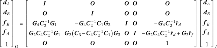
As shown in Figure 11.5, a general multibody system is regarded as a system composed of a tree subsystem and some closed‐loop subsystems. After cutting at the junction between body 2 and hinge 19, a couple of new boundaries with equivalent state vectors, signed as z2,0 and z19,0, are generated at the cutting point, as shown in Figure 11.6. The former nontree system has changed to a tree system with two new boundary state vectors z2,0 and z19,0 at the cutting point. Thus, according to section 11.4, the overall transfer equation of a general system composed of closed‐loop subsystems and tree subsystems can be derived manually or by computer.
Figure 11.5 Topology figure of a nontree system.
Figure 11.6 Topology figure of a tree system generated by a nontree system after cutting hinge 19.
It should be noted that both z2,0 and z19,0 are the input ends of some elements (here the input ends of elements 2 and 19, respectively), therefore the internal forces and internal moments in z2,0 and z19,0 are equal in magnitude and opposite in direction according to sign conventions, that is
where
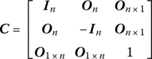
is the cutting point sign convention matrix in this book, where n is equal to 3 or 6 for planar motion or spatial motion, respectively.
For tree systems, taking the relation expression of z2,0 and z19,0, namely Equation (11.28), into account, the overall transfer equation of a general multibody system, as shown in Figure 11.6, with closed‐loop subsystems can be derived automatically by handwriting or by computer,
where

Considering that z19,0 can be described by z2,0 using Equation (11.28), the overall transfer equation, the overall transfer matrix and the system boundary state vector of the general system can be written as
where


Equations (11.32) to (11.34) show that as long as the state vectors of each pair of cutting points are the same and comply with sign conventions, the forms of the overall transfer equation, the main transfer equation and the geometric equation of a general system that consists of closed‐loop subsystems and a tree subsystem are identical as those of the tree system developed by cutting the closed‐loop subsystem. In this book, the original system boundary state vectors and all the body element end state vectors at the cutting point are defined as augmented boundary state vectors.
11.6 Automatic Deduction Theorem of the Overall Transfer Equation
Owing to the deduction process introduced in sections 11.3–11.5, the following characteristics of the multibody system transfer equation are found, by which the automatic deduction theorem of the overall transfer equation of closed‐loop systems, tree systems and general systems can be developed.
- The state vector involved in the overall transfer equation, zall, is referred to as the system boundary state vector. The coefficient matrix of the system boundary state vector is the overall transfer matrix Uall of the system.
- For tree systems the overall transfer equation includes the main transfer equation and geometric equations. The coefficient matrix of the system boundary state vector in the main transfer equation corresponds to the first row of the overall transfer matrix, in which the coefficient matrix of the root state vector is the minus identity matrix. The coefficient matrix of the main transfer equation, that is, the coefficient matrix T of the branch state vector, has a structure with the following rules: the coefficient matrix of each branch state vector is the successive multiplication of the transfer matrices of all the elements from branch to root along the transfer route.
As for the geometric equations of the tree system, if a branch terminates at the first input end of a multiple‐input element, then the corresponding coefficient is obtained by successive multiplication of the transfer matrices of all elements along this path and by a final premultiplication of the corresponding negative position extraction matrix. Likewise, if a branch terminates at a nonfirst input end of a multiple‐input element, then the corresponding coefficient is obtained by successive multiplication of the transfer matrices of all elements along this path and by a final premultiplication of the corresponding positive position extraction matrix.
- For a chain system, any chain system can be regarded as a special case of a tree system which has only two boundaries. No geometric equations are involved for a chain system. In addition, the automatic deduction theorem (b) of the overall transfer equation for tree systems is also valid for chain systems.
- For a closed‐loop system, by cutting the loop into a chain the original system can be regarded as a chain system. The automatic deduction theorem (b) of the overall transfer equation for tree systems is also valid for closed‐loop systems.
- For a general system composed of a tree subsystem and a closed‐loop subsystem, by cutting off the closed loops, the original system can be changed to a tree system with the boundary ends corresponding to the cutting points. Therefore, the forms of the overall transfer equation, the main transfer equation and the geometric equation in general systems with closed‐loop subsystems and tree subsystems are the same as in tree systems formed by cutting the closed‐loop subsystems.
The above automatic deduction theorem of the overall transfer equation of multibody systems applies for a variety of MRSs, chain multi‐rigid‐flexible‐body systems (MRFSs), closed‐loop MRFSs, tree MRFSs and general MRFSs in which a body element with more than two ends is assumed to be a rigid body, and has laid a foundation for building large‐scale MSD software with high computing speed.
11.7 Numerical Example of Closed‐loop System Dynamics
11.7.1 Vibration Characteristics of a Closed‐loop Multibody System
For a closed‐loop MRFS, the sequence number of the first element is the same as that of the end element, thus it can be regarded as a chain system if the system is “cut” at a connection point. The multibody dynamic problems of closed‐loop systems can be studied using the MSTMM.
For example, Figure 11.7 shows a closed‐loop system composed of three lumped masses and three springs. A connection point can be defined as the input end of the system, and at the same time it is the output end of the system. Each element is numbered successively along the loop. The transfer direction can be defined arbitrarily. The following discussion is based on the sequence numbers shown in Figure 11.7.
Figure 11.7 A closed‐loop system composed of lumped masses and springs.
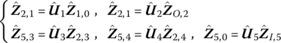
The state vectors Z6,1, Z2,1, Z2,3, Z4,3, Z4,5 and Z6,5 are defined as ![]() . The transfer equations are
. The transfer equations are
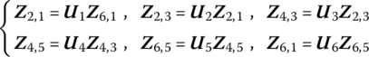
The transfer matrices have already been given in Equations (2.13) and (2.19), and thus are omitted here. According to Equation (11.38), we obtain
Equation (11.39) is the overall transfer equation of the system, which can be written as
The elements of Z6,1 are all unknown because Z6,1 is not the state vector at the boundary point but the state vector at the connection point, that is
Therefore, the characteristic equation is obtained as
The closed‐loop MRFS shown in Figure 11.8 is composed of four elastic beams and four rigid bodies. The transverse and longitudinal vibrations of the beams are considered in a plane. The sequence number of each element is shown. The state vectors Z8,1, ![]() , Z2,1, Z2,3,
, Z2,1, Z2,3, ![]() , Z4,3, Z4,5,
, Z4,3, Z4,5, ![]() , Z6,5, Z6,7,
, Z6,5, Z6,7, ![]() and Z8,7 are defined in the form of
and Z8,7 are defined in the form of ![]() , where Z8,1,
, where Z8,1, ![]() and Z2,1 are defined in the coordinate system I1x1y1, Z2,3,
and Z2,1 are defined in the coordinate system I1x1y1, Z2,3, ![]() and Z4,3 are defined in the coordinate system I3x3y3, Z4,5,
and Z4,3 are defined in the coordinate system I3x3y3, Z4,5, ![]() and Z6,5 are defined in the coordinate system I5x5y5, and Z6,7,
and Z6,5 are defined in the coordinate system I5x5y5, and Z6,7, ![]() and Z8,7 are defined in the coordinate system I7x7y7.
and Z8,7 are defined in the coordinate system I7x7y7.
Figure 11.8 A closed‐loop system of a multi‐rigid‐flexible‐body.
The transfer equation of element 1 in the coordinate system I1x1y1 is
where U1 is the transfer matrix of beam 1.
The state vectors Z2,1 at the input end and Z2,3 at the output end of rigid body 2 are defined in the two different coordinate systems I1x1y1 and I3x3y3, respectively. The orientation discrepancy of the two coordinate systems is 90°. As a result, a coordinates transformation has to be made in the transfer equation of rigid body 2, that is
where

U2 is the transfer matrix of rigid body 2 and H is the coordinate transformation matrix.
Similarly, we can obtain
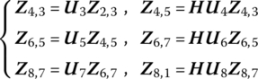
According to Equations (11.43) to (11.45), the overall transfer equation is obtained
that is
The characteristic equation is
The natural frequencies ![]() of the system can be determined by solving Equation (11.47), and Z8,1 is obtained by Equation (11.46). The state vectors at each point can be evaluated by the transfer equations of every element. Since the state vectors are not defined in the same coordinate system, they must be transformed to the common coordinate system oxyz when computing the mode shapes by the state vectors. Because the orientation of I1x1y1 is the same as the orientation of oxyz, Z8,1,
of the system can be determined by solving Equation (11.47), and Z8,1 is obtained by Equation (11.46). The state vectors at each point can be evaluated by the transfer equations of every element. Since the state vectors are not defined in the same coordinate system, they must be transformed to the common coordinate system oxyz when computing the mode shapes by the state vectors. Because the orientation of I1x1y1 is the same as the orientation of oxyz, Z8,1, ![]() and Z2,1 need not be transformed. The others need to be transformed according to the following relations:
and Z2,1 need not be transformed. The others need to be transformed according to the following relations:
where

11.7.2 Dynamics of a Closed‐Loop Multibody System
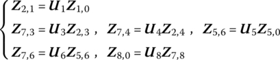
The closed‐loop multibody system shown in Figure 11.9 can be regarded as a chain system with the same input and output state vectors. Hence
where
Figure 11.9 A closed‐loop multibody system.
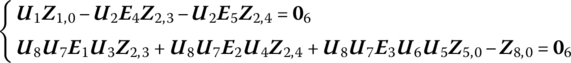
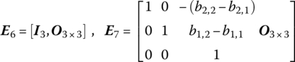
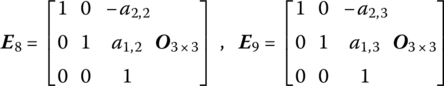
The overall transfer equation of the system is
and the overall transfer matrix of the system is
It can be seen that the solution process of a closed‐loop multibody system using the MSDTTMM is as easy as for a chain multibody system.
For the closed‐loop multibody system shown in Figure 11.10, we obtain

where
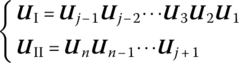
Figure 11.10 A multibody system with a closed‐loop structure.
The boundary conditions are

If element j is a smooth hinge, according to the continuous condition of position coordinate and the equilibrium of forces, we can obtain
Hence,
The overall transfer equation of the system is
The overall transfer matrix of the system is
11.8 Numerical Example of Tree System Dynamics
11.8.1 Vibration Characteristics of Tree Systems
For a branched MRFS, the MSTMM is very effective. To study the dynamic problems of a branched MRFS, the solution steps are the same as for the chain system. For each connection point, the geometric equations and the equilibrium equations need to be formulated according to the geometric relations and equilibrium conditions, respectively.
11.8.1.1 Another Form of Characteristic Equation
If the number of elements in a chain system is n, the overall transfer equation of the system is
which can be written as
Let ![]() and
and ![]() . Then Equation (11.69) turns into
. Then Equation (11.69) turns into
Zall is composed of Z1,0 and Zn,0, which are both state vectors at the boundary of the system, and half of the elements in Zall are zeros according to the boundary conditions. We delete the null elements of Zall and define the column vector composed of the remainder as ![]() . At the same time we delete the corresponding columns of Uall and define the remainder as
. At the same time we delete the corresponding columns of Uall and define the remainder as ![]() , which is a square matrix, thus
, which is a square matrix, thus
![]() is composed of the unknown elements. If the homogeneous equation has a nonzero solutions, there must be
is composed of the unknown elements. If the homogeneous equation has a nonzero solutions, there must be
Equation (11.72) is another form of the characteristic equation. It can be proved that the equation has the same solutions as the characteristic equation ![]() obtained from
obtained from ![]() in the chain system, but the order number of
in the chain system, but the order number of ![]() is higher than that of U′. We can obtain U′ in the chain system. For other complex systems, we cannot obtain U′, only
is higher than that of U′. We can obtain U′ in the chain system. For other complex systems, we cannot obtain U′, only ![]() .
.
11.8.1.2 Characteristic Equation of a Tree System
The branched MRFS in Figure 11.16 is composed of two elastic hinges, two rigid bodies and a beam with a uniform cross‐section vibrating in a plane. It also has three boundary points. The right‐hand side of the beam is defined as the output end of the system, and the other two boundary points are input ends. Let the point connected with the ground be the first input end, and the other point be the second input end.
Figure 11.16 A branched MRFS.
The sequence numbers of the elements are shown in Figure 11.16, and the system is composed of five elements, that is, ![]() , in two transfer directions. The elements are numbered 5, 4, 3 and 2 sequentially along the direction from the output end to the second input end. The elastic hinge between element 4 and the ground is numbered 1, the boundaries at both input ends are numbered 0 and the boundary at the output end is numbered
, in two transfer directions. The elements are numbered 5, 4, 3 and 2 sequentially along the direction from the output end to the second input end. The elastic hinge between element 4 and the ground is numbered 1, the boundaries at both input ends are numbered 0 and the boundary at the output end is numbered ![]() . The state vectors Z1,0, Z4,1, Z2,0, Z2,3, Z4,3, Z4,5,
. The state vectors Z1,0, Z4,1, Z2,0, Z2,3, Z4,3, Z4,5, ![]() and Z5,0 are defined in the form of
and Z5,0 are defined in the form of ![]() , therefore the transfer equations are
, therefore the transfer equations are
where U1 and U3 are the transfer matrices of the planar elastic hinges, U2 is the transfer matrix of the rigid body with one input end and one output end, and U5 is the transfer matrix of a beam with transverse and longitudinal vibrations.
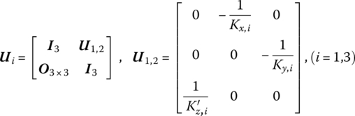
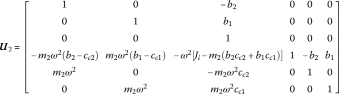

Here (b1, b2) and (cc1, cc2) are the position coordinates of the output end and mass center, respectively, in the body‐fixed coordinate system in which the input end is the origin, ![]() and
and ![]() .
.
Element 4 is a rigid body with two input ends and one output end, and the state vectors are Z4,1 and Z4,3 at the two input ends. The state vector ZI,4 at the input end is defined as
where

Therefore, the transfer equation of element 4 is
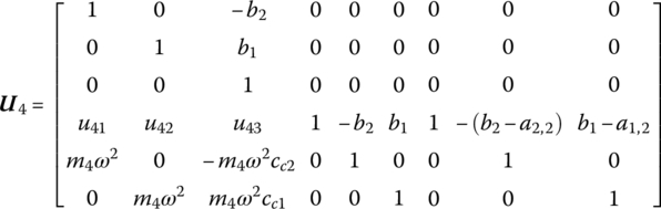
where (b1, b2) and (cc1, cc2) are the position coordinates of the output end and the mass center of rigid body 4 in the body‐fixed coordinate system, respectively, and the first input end is the origin of the body‐fixed coordinate system. (a1,2, a2,2) are the position coordinates of the second input end of rigid body 4 in the body‐fixed coordinate system, and the detailed expressions of u41, u42 and u43 are ![]() ,
, ![]() and
and ![]() , respectively.
, respectively.
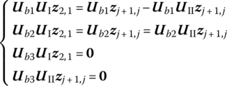
According to Equations (11.73), (11.74) and (11.78), we have
that is
In addition, there are relations between the three elements denoting the displacement in Z4,3 and Z4,1, that is
where

therefore
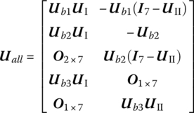
Combining Equations (11.80) and (11.82) yields
where

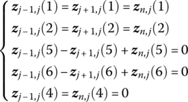
According to the boundary conditions

The 1st, 2nd, 3rd, 10th, 11th, 12th, 16th, 17th and 18th elements of Zall are zero. These null elements are deleted from Zall and the corresponding columns are deleted from Uall, therefore
The characteristic equation is
11.8.1.3 Mode Shapes of Tree Systems
The natural frequencies ![]() of the system can be obtained by solving Equation (11.86). For each ωk the corresponding boundary state vectors Z1,0, Z2,0 and Z5,0 can be determined by solving Equation (11.85). Consequently, the state vectors of the other connection points can be evaluated, and the state vectors at arbitrary positions of the beam can be computed from the transfer equation
of the system can be obtained by solving Equation (11.86). For each ωk the corresponding boundary state vectors Z1,0, Z2,0 and Z5,0 can be determined by solving Equation (11.85). Consequently, the state vectors of the other connection points can be evaluated, and the state vectors at arbitrary positions of the beam can be computed from the transfer equation ![]() . Thus, the mode shape of the system is acquired. When solving the vibration characteristics of the tree system, the method is the same as that of the chain system, and both have the same procedure.
. Thus, the mode shape of the system is acquired. When solving the vibration characteristics of the tree system, the method is the same as that of the chain system, and both have the same procedure.
11.8.2 Dynamics of Tree Multibody Systems
11.8.2.1 Solve the Steady‐state Response of an MRFS under Harmonic Excitation using the Extended MSTMM
Some simple chain systems were discussed in Chapter 2. The general systems will be studied using this method in the following.
The planar MRFS shown in Figure 11.18 is composed of two rigid bodies and three elastic hinges. The elastic hinges have viscous damping with coefficients ![]() , respectively, along the x and y directions as well as rotation about the z direction. Two rigid bodies are excited to harmonic forces acting on points D2 and D5:
, respectively, along the x and y directions as well as rotation about the z direction. Two rigid bodies are excited to harmonic forces acting on points D2 and D5:

Figure 11.18 Planar MRFS composed of two rigid bodies and three elastic hinges.
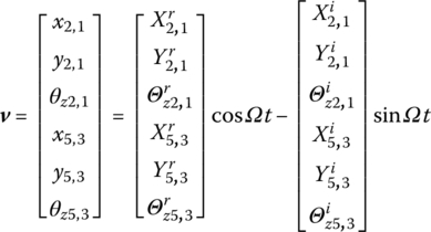
The external force is expressed in the complex form ![]() , then
, then
therefore
namely
The extended state vectors ![]() 1,0,
1,0, ![]() 2,1,
2,1, ![]() 2,3,
2,3, ![]() 2,4,
2,4, ![]() 5,3,
5,3, ![]() 5,4 and
5,4 and ![]() 5,0 are defined as
5,0 are defined as
The state vectors ![]() O,2 and
O,2 and ![]() I,5 are
I,5 are
where

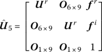
The extended transfer equation of each element is
where ![]() ,
, ![]() and
and ![]() are the extended transfer matrices of hinges 1, 3 and 4, respectively.
are the extended transfer matrices of hinges 1, 3 and 4, respectively.![]() is the extended transfer matrix of a rigid body with one input and two output ends,
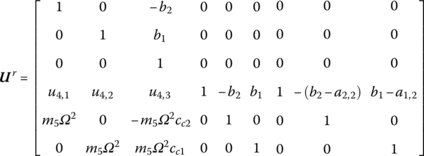
is the extended transfer matrix of a rigid body with one input and two output ends, ![]() is the extended transfer matrix of a rigid body with two input ends and one output end
is the extended transfer matrix of a rigid body with two input ends and one output end


where ![]() and (d1, d2) denotes the coordinates of point D2 in the body‐fixed coordinate system of rigid body 2.
and (d1, d2) denotes the coordinates of point D2 in the body‐fixed coordinate system of rigid body 2.
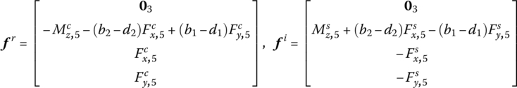
where ![]() ,
, ![]() and
and ![]() , and (d1, d2) denotes the coordinates of point D5 in the body‐fixed coordinate system of rigid body 5.
, and (d1, d2) denotes the coordinates of point D5 in the body‐fixed coordinate system of rigid body 5.
According to Equation (11.83),

According to the geometrical relationship between different ends of body 2, we have
where
Similarly, we obtain
where

Substituting the part transfer equations of Equation (11.92) into Equation (11.98) yields
Combining Equation (11.96) with Equation (11.99) and rewriting in the form of a matrix
According to boundary conditions, we obtain
Thus, the 1st, 2nd, 3rd, 7th, 8th, 9th, 17th, 18th, 19th, 23rd, 24th and 25th variables in Zall are all zero, meanwhile the 13th, 26th, 39th and 52nd variables are equal to 1. These known elements are removed from Zall, and the columns corresponding to each zero element are removed from Uall. Move the columns corresponding to all nonzero elements to the right‐hand side of the equation and cancel the 13th and 26th rows in Equation (11.100). Then
where
and ui,j is the variable in the i th row and j th column in Uall.
With the inverse of Ûall, Equation (11.102) becomes
Then the unknown state variables in Zall are obtained. ![]() ,
, ![]() ,
, ![]() ,
, ![]() ,
, ![]() ,
, ![]() and
and ![]() ,
, ![]() ,
, ![]() ,
, ![]() ,
, ![]() ,
, ![]() can be determined using transfer equations of elements. With
can be determined using transfer equations of elements. With ![]() , this becomes
, this becomes
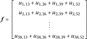
therefore the steady‐state response of the system is obtained
The exact value of a particular solution is obtained using the MSTMM in the above example, and the computational effort is greatly reduced.
11.8.2.2 Static Response of a Multibody System
11.9 Numerical Example of Multi‐level System Dynamics
A system is comparative of the principal system, as shown in Figure 11.26. A multi‐level MRFS or multi‐layer system has several layers superposed, and each branch is a subsystem connected with the adjacent subsystems.
Figure 11.26 Multi‐level MRFS.
Assuming the state vectors at each layer are ![]() ,
, ![]() , …,
, …, ![]() , respectively, the state vector of a whole column is
, respectively, the state vector of a whole column is
If the transfer matrices of each layer are ![]() ,
, ![]() ,
, ![]() ,
, ![]() , the transfer equation of a whole column is
, the transfer equation of a whole column is

In the subsystem, the transfer matrix at a certain point is introduced by a simple basic example of a two‐level system as follows.
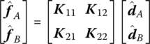
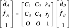
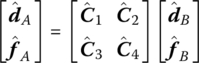
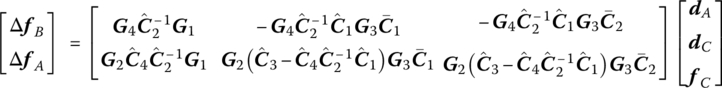
For the two‐level system AB shown in Figure 11.27, the transfer equation related to layers A and B is
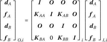
where the vectors ![]() and
and ![]() denote displacements and forces, respectively, and subscripts I and O denote the input and output ends, respectively. Furthermore, subscripts A and B denote the corresponding quantities on layers A and B, respectively.
denote displacements and forces, respectively, and subscripts I and O denote the input and output ends, respectively. Furthermore, subscripts A and B denote the corresponding quantities on layers A and B, respectively. ![]() ,
, ![]() ,
, ![]() and
and ![]() are the elastic matrices, and the computational method is as follows.
are the elastic matrices, and the computational method is as follows.
Figure 11.27 Subsystem of a two‐level system.
11.9.1 Derivation of an Elastic Matrix from the Stiffness Matrix of a Subsystem
The stiffness matrix of a subsystem can be given in the coordinates of a subsystem, that is
The elastic matrix of Equation (11.105) is obtained as follows
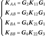
where ![]() ,
, ![]() ,
, ![]() and
and ![]() are coordinate transformation matrices.
are coordinate transformation matrices.
11.9.2 Derivation of an Elastic Matrix from the Transfer Matrix of a Subsystem
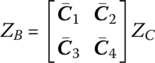
The transfer equation of the subsystem is

Solving it, we obtain
The coordinate transformation from the subsystem to the principal system yields
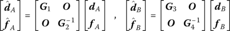
From the equations above, the forces at layers A and B are expressed by their displacement in the principle system

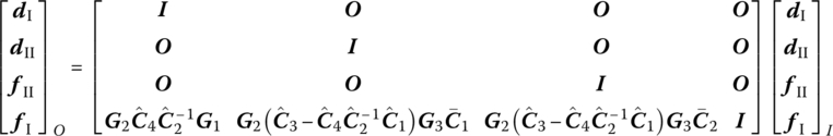
therefore the transfer equation is

According to the expanded transfer matrix
After transforming the coordinate, the expanded transfer equation of the subsystem is obtained
11.9.3 Two‐level Parallel System with Nonvertical Connection
As shown in Figure 11.28, the two‐level parallel system is connected in a slanted direction by the subsystem. It is assumed that the connection of nodes A and B is a stiffness connection. The displacement is continuous, but the internal force is discontinuous. In local coordinates of the subsystem, the state vectors of the ends of nodes A and B have the following relations
where ![]() and
and ![]() express the displacement and internal force of vectors in local coordinates, respectively.
express the displacement and internal force of vectors in local coordinates, respectively.
In the whole coordinate belong to the principal systems ![]() and
and ![]() , the increment of internal force at nodes A and B can be expressed by their displacements
, the increment of internal force at nodes A and B can be expressed by their displacements

where ![]() ,
, ![]() ,
, ![]() and
and ![]() are the transformation matrices of the displacements and the internal forces at nodes A and B from the local coordinate system to the principal coordinate system.
are the transformation matrices of the displacements and the internal forces at nodes A and B from the local coordinate system to the principal coordinate system.
The transfer equation from C to B in principal system ![]() is
is
therefore
Figure 11.28 Two‐level parallel system with nonvertical connection.
Substituting Equation (11.150) into Equation (11.149) yields
Considering the continuity of displacements and internal forces without subsystem AB, the transfer equation of principal systems ![]() and
and ![]() can be obtained at section AC as
can be obtained at section AC as
Similarly, the transfer equation of principal systems ![]() and
and ![]() at section BD is
at section BD is

where ![]() and
and ![]() are submatrices of the transfer matrices in principal system
are submatrices of the transfer matrices in principal system ![]() from D to A.
from D to A.
11.10 Numerical Example of General System Dynamics
11.10.1 Vibration Characteristics of a Hybrid Multibody System with a Branched and Closed‐loop System
A hybrid MRFS with a branched and closed‐loop system only needs to build geometric relation equations and equilibrium equations according to the displacement geometric conditions and equilibrium conditions in each connection point, respectively, and the other steps of the solution are the same as those in the chain system. The MSTMM can expediently solve the dynamic problems of the hybrid MRFS with a branched and closed‐loop system.
Figure 11.29 shows a hybrid MRFS with a branched and closed‐loop system vibrating in a plane. The elements 1, 3, 4 and 6 are planar elastic hinges, elements 2, 5 and 7 are rigid bodies, and element 8 is an elastic beam. The sequence number of the elements is shown in Figure 11.29. The free end of the beam is defined as the output end of system. The connection point between element 1 and the ground is defined as the first input end of system, and the free end of element 5 is defined as the second input end of the system.
Figure 11.29 A hybrid MRFS with a branched and closed‐loop system.
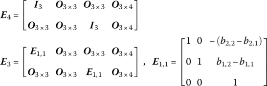
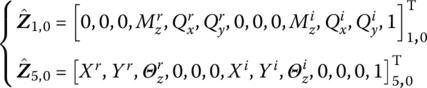
The state vectors ![]() ,
, ![]() ,
, ![]() ,
, ![]() ,
, ![]() ,
, ![]() ,
, ![]() ,
, ![]() ,
, ![]() ,
, ![]() ,
, ![]() and
and ![]() can be defined in the form of
can be defined in the form of ![]() .
.
Element 7 is a rigid body with three input ends and one output end. Its three state vectors at the input ends are ![]() ,
, ![]() and
and ![]() . The state vector
. The state vector ![]() at the input end is defined as
at the input end is defined as
where
The transfer equation is
The transfer matrix is
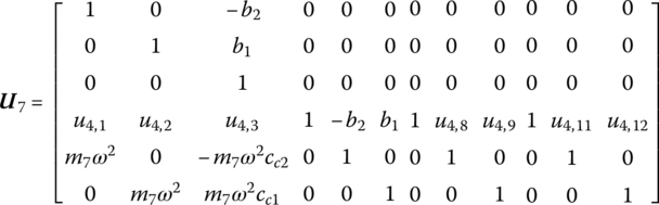
where

(b1, b2) and (cc1, cc2) are the position coordinates of the output end and the mass center of rigid body 7, respectively, in the body‐fixed coordinate system in which the first input end is the origin. (a1,2, a2,2) and (a1,3, a2,3) are the position coordinates of the second and third input ends, respectively, of rigid body 7 in the body‐fixed coordinate system.
Element 2 is a rigid body with one input end and two output ends, and its two state vectors at the output ends are ![]() and
and ![]() . The state vector
. The state vector ![]() of the output end is defined as
of the output end is defined as
where
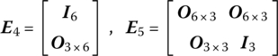
The transfer equation is
The transfer matrix is
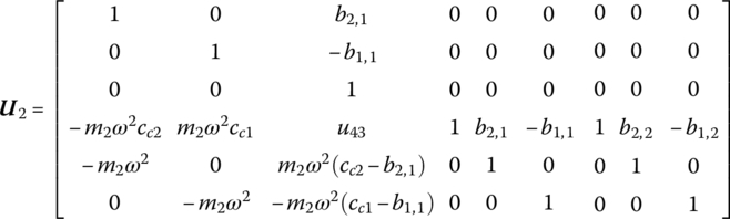
where
(b1,1, b2,1) and (b1,2, b2,2) are the position coordinates of the two output ends of rigid body 2 in the body‐fixed coordinate system, whose input end is the origin.
The transfer equations of the other elements are
where ![]() ,
, ![]() ,
, ![]() and
and ![]() are the transfer matrices of hinges 1, 3, 4 and 6, respectively,
are the transfer matrices of hinges 1, 3, 4 and 6, respectively, ![]() is the transfer matrix of a rigid body with one input and one output end, and
is the transfer matrix of a rigid body with one input and one output end, and ![]() is the transfer matrix of the beam.
is the transfer matrix of the beam.
According to Equations (11.155), (11.157) and (11.158), we obtain
![]() and
and ![]() are both state vectors of rigid body 2, where the six elements denoting displacement are linear correlative
are both state vectors of rigid body 2, where the six elements denoting displacement are linear correlative
where
Similarly, both ![]() and
and ![]() are state vectors of rigid body 7. The dependent displacements can be expressed linearly by three independent displacements in state vector
are state vectors of rigid body 7. The dependent displacements can be expressed linearly by three independent displacements in state vector ![]() at the first input end of element 7
at the first input end of element 7
where
In the body‐fixed coordinate system, (a1,2, a2,2) and (a1,3, a2,3) are the position coordinates of the second and third input ends of rigid body 7.
According to Equations (11.158) and (11.161), we obtain

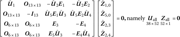
Combining Equations (11.159), (11.160) and (11.162), the matrix form is
where

According to the boundary conditions, we obtain

therefore elements 1, 2, 3, 10, 11, 12, 16, 17 and 18 in ![]() are zeros. These null elements are deleted from
are zeros. These null elements are deleted from ![]() , and the corresponding columns are deleted from
, and the corresponding columns are deleted from ![]() . We obtain
. We obtain ![]() , and the characteristic equation is
, and the characteristic equation is ![]() .
.
It is important to note that both the state vectors at connection points ![]() and
and ![]() are contained in
are contained in ![]() . This is different from the case where
. This is different from the case where ![]() contains only state vectors at the boundary points, as mentioned before. This is caused by the closed loop in the system. The overall transfer equation of a closed‐loop system does not contain state vectors at any boundary points, but only contains state vectors at the interior connection points.
contains only state vectors at the boundary points, as mentioned before. This is caused by the closed loop in the system. The overall transfer equation of a closed‐loop system does not contain state vectors at any boundary points, but only contains state vectors at the interior connection points.
The state vectors at interior connection points may linearly depend on the state vectors at the boundary points, but from knowledge of linear algebra this does not affect the solution of the characteristic equation and ![]() . In this system,
. In this system, ![]() and
and ![]() of Equation (11.163) can be substituted by
of Equation (11.163) can be substituted by ![]() . Consequently, the order of the overall transfer equation and the overall transfer matrix can be decreased to three. We can even make
. Consequently, the order of the overall transfer equation and the overall transfer matrix can be decreased to three. We can even make ![]() and
and ![]() disappear in
disappear in ![]() by skillful transformation, which will greatly decrease the order of the overall transfer equation and the overall transfer matrix. The details are discussed below.
by skillful transformation, which will greatly decrease the order of the overall transfer equation and the overall transfer matrix. The details are discussed below.
The transformation relation from ![]() and
and ![]() to
to ![]() is established in Equation (11.157), while the transformation relations from
is established in Equation (11.157), while the transformation relations from ![]() to
to ![]() and
and ![]() are transformed as follows
are transformed as follows
where
Equation (11.165) can be substituted into Equations (11.159) and (11.162), and the matrix form written as
where

Thus, we can obtain ![]() . There are only 18 unknown elements in
. There are only 18 unknown elements in ![]() and three less than before, so the order of
and three less than before, so the order of ![]() is correspondingly reduced by three.
is correspondingly reduced by three.
If Equation (11.159) is rewritten as
that is

we obtain

We can define

then
Substituting Equation (11.171) into Equations (11.160) and (11.162), and writing them in matrix form gives
where

Thus, there are only nine unknown elements in ![]() . Correspondingly,
. Correspondingly, ![]() is a square matrix with order 9, and its order is greatly reduced.
is a square matrix with order 9, and its order is greatly reduced.
11.10.2 Dynamics of a Network Multibody System
11.10.3 Dynamics of General Multibody System
A general multi‐rigid‐body system containing a close loop moving in a plane is shown in Figure 11.33. The planar rigid bodies (numbered 1, 3, 5, 7, 9, 11 and 13) are connected by pin hinges (numbered 2, 4, 6, 8, 10, 12 and 14), and rigid body 1 is connected with the ground by a smooth pin. Each rigid body has the identical dynamics parameters
Figure 11.33 A general system moving in a plane.
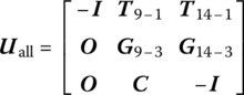
By “cutting” at the junction of body 9 and hinge 14, and following the proposed theorem, the topology figure of the system can be drawn, as shown in Figure 11.34. The overall transfer equation of the system can be derived automatically as
where the overall transfer matrix takes the form
The state vectors of all the boundary ends are

According to the proposed sign conventions, we obtain


z1,0 is the state vector of the root, z9,0 and z14,0 are the state vectors of the tips that emerge after the cutting. ![]() , U3, U3,10, U5, U7, U9, U11 and U13 are the transfer matrices of the corresponding planar rigid bodies. U2, U4, U6, U8, U10, U12 and U14 are the transfer matrices of the corresponding planar pin hinges.
, U3, U3,10, U5, U7, U9, U11 and U13 are the transfer matrices of the corresponding planar rigid bodies. U2, U4, U6, U8, U10, U12 and U14 are the transfer matrices of the corresponding planar pin hinges.
The boundary conditions of the system are
Figure 11.34 Topology figure of the general system moving in a plane.
The initial angle of the rigid body 1 is π/6 rad and the relative angles of the pin hinges (numbered 2, 4, 6, 8, 10, 12 and 14) are all zero. The system moves from rest under the effect of gravity. The computational results of the system dynamics are obtained by the proposed method and by the Newton–Euler method. The time history of the angle of rigid body 1 is given in Figure 11.35, which shows that the computational results obtained by the two methods are in good agreement.
Figure 11.35 Computational results of the angle of rigid body 1.