
7
Discrete Time Transfer Matrix Method for Multibody Systems
7.1 Introduction
7.1.1 Characteristics of Ordinary Multibody System Dynamics Methods
With the development of modern industrial technology, many complex mechanical systems have appeared, such as weaponry, aeronautics, astronautics, vehicles, robots and precision machines, which are composed of many components with large relative motion. Under the condition of strong engineering demands, a new branch, namely multibody system dynamics, appeared. The numerical simulation of complex mechanical systems became possible with the appearance and development of the computer. Multibody system dynamics is an engineering application essential to the study of mechanical system dynamics, and systems consisting of many bodies undergoing large relative motion are its main study object. In general, the components of multibody systems include bodies and joints. Body components include rigid bodies, flexible bodies and lumped masses. A system is a multi‐rigid‐body system if the bodies involved are all rigid bodies, it is a multi‐flexible‐body system if the bodies involved are all flexible bodies and a multi‐rigid‐flexible‐body system if both rigid bodies and flexible bodies are involved. The joints are the components connecting the bodies.
The deduction of the dynamic equations of multibody systems and their numerical solutions are two main research areas of multibody system dynamics. Generally, there are two major methods for deriving dynamic equations, and their basic forms are different. The first method uses Lagrangian equations of the first kind, in which Lagrange multipliers are used to define unknown generalized constraint forces and obtain an augmented formulation. This approach leads to a mixed set of nonlinear differential and algebraic equations that have to be solved simultaneously, and it is the theoretical foundation of some commercial analysis software, such as ADAMS and DADS. It must solve a set of differential‐algebraic equations. The second method describes the motion using a set of first‐order differential equations (kinematics and dynamics) with a minimal set of unknown variables without constraint forces. From a point of view of computational efficiency, its numerical solution is more sophisticated. Differential‐algebraic equations can be transformed into a new form with a minimal number of coordinates, and a typical code is the MBOSS [246] developed by Arizona University.
With developments in engineering technology, researchers are still proposing and improving various multibody system dynamics methods, which are promoting the development of modern engineering technology. These methods have different forms, but in general they all have the two same characteristics:
- It is necessary to build the global dynamic equations of the system, which is the most interesting and brilliant part of various methods, but is also the difficult part for engineers.
- The orders of matrices involved in the global dynamic equations of the system are rather high (generally speaking not less than the degrees of freedom (DOFs) of the system). It has become one of the main research directions in multibody system dynamics to search for a new method to reduce the orders of relevant matrices and to avoid computational difficulty caused by high matrix order.
7.1.2 Features of the Discrete Time Transfer Matrix Method for Multibody Systems
To improve the computational efficiency of multibody system dynamics, a new method, the discrete time transfer matrix method for multibody systems (MSDTTMM) [3, 64–68], has been developed, which is different from other ordinary methods of multibody system dynamics. This method combines the advantages of the transfer matrix method and numerical integration. The dynamics equations of typical elements are derived first, followed by their discretization and linearization in the time domain based on the basic thought of numerical integration. Then the transfer matrices of these elements are obtained. The overall transfer equation and overall transfer matrix of the multibody system can be assembled. The system motion can be obtained using step‐by‐step time integration. The method is suitable for linear time‐variable, nonlinear, large motion and general multibody systems. Compared with ordinary multibody system dynamics methods, the MSDTTMM has the following features:
- The global dynamic equations of a system are not needed, hence its application and computation are very convenient.
- The order of involved matrices is much lower than for ordinary multibody system dynamics methods. For example, the order of relevant matrices for chain multibody systems is determined only by the highest order of differential equations of its subsystems. The computational cost is small, resulting in high computational efficiency.
- It provides a flexible modeling instrument and the modeling procedure is highly programmable. The modeling of a multibody system looks like building blocks, the overall transfer matrix of the system can be assembled by the transfer matrices of each element directly, and its solution procedure is very simple and straightforward.
- Complex multibody systems, such as branch, closed‐loop or network systems, can be conveniently dealt with by this method in a similar way to the transfer matrix method for linear multibody systems.
- The study method for multi‐flexible‐body systems and the MRFS is the same as that for multi‐rigid‐body systems.
- The transfer matrix is always a real number matrix, even when considering dampers. This simplifies the numerical algorithm.
- The natural frequency of linear multibody systems can be obtained easily by using the MSDTTMM, and the transfer matrix method for linear multibody systems can be regarded as a special case.
- An arbitrary appropriate numerical integration method can be introduced into the MSDTTMM, which gives the method some flexibility.
The basic principles, steps and algorithm of the MSDTTMM developed by the authors are introduced in this chapter, and the transfer matrices of typical elements are deduced.
7.2 State Vector, Transfer Equation and Transfer Matrix
Enlightened by the idea of matrix “transfer” in the transfer matrix method for linear time‐invariant systems, the concepts of state vector, transfer equation and transfer matrix for nonlinear time‐variant systems are introduced in this section. These new concepts are not the same as those in the transfer matrix method for linear time‐invariant systems. We start to address these concepts with a simple example.
Figure 7.1 shows a chain multi‐DOF system composed of springs and lumped masses moving along the ox axis. As shown in Figure 7.2, each spring and the lumped mass on its right can be regarded as a subsystem. The position coordinate of the left side of spring j is denoted by ![]() , the corresponding force is denoted by
, the corresponding force is denoted by ![]() . Their positive direction is the same as the positive direction of the ox axis, and the position coordinate of the right side of spring j is denoted by
. Their positive direction is the same as the positive direction of the ox axis, and the position coordinate of the right side of spring j is denoted by ![]() , the force is denoted by
, the force is denoted by ![]() and their positive direction is the same as the negative direction of the ox axis. For a massless spring, we have
and their positive direction is the same as the negative direction of the ox axis. For a massless spring, we have
and for a linear spring, according to Hooke’s law, we obtain
where lj is the initial length of the spring and Kj is the stiffness coefficient.
Figure 7.1 A chain system with multiple DOFs.
Figure 7.2 Subsystem model.
For lumped mass ![]() , the position coordinate of its left side is denoted by
, the position coordinate of its left side is denoted by ![]() and the corresponding force denoted by
and the corresponding force denoted by ![]() . Their positive direction is the same as the positive direction of the ox axis, and the position coordinate of its right side is denoted by
. Their positive direction is the same as the positive direction of the ox axis, and the position coordinate of its right side is denoted by ![]() . The force is denoted by
. The force is denoted by ![]() and the positive direction is the same as the negative direction of the ox axis. According to Newton’s second law of motion, we obtain
and the positive direction is the same as the negative direction of the ox axis. According to Newton’s second law of motion, we obtain
where ![]() is the mass of body
is the mass of body ![]() and
and ![]() is the external force acting on the body.
is the external force acting on the body.
There are many numerical methods which describe ![]() and
and ![]() as linear functions of x. For example, by using the Taylor series, we find
as linear functions of x. For example, by using the Taylor series, we find
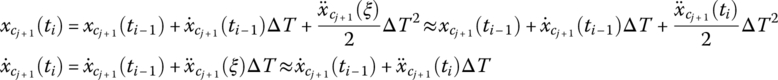
![]() and
and ![]() can be expressed as linear functions of
can be expressed as linear functions of ![]() :
:
where ![]() is a time step.
is a time step.
Substituting Equation (7.4) into Equation (7.3) yields
According to the continuous condition of displacement of lumped mass, this becomes
Combining Equations (7.1) and (7.2) yields
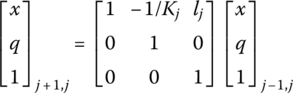
The state vector at the connection point is defined as
Equation (7.8) can be written as
where

Equation (7.8) or Equation (7.10) is the transfer equation of a spring, and Equation (7.11) is the transfer matrix of a spring. Combining Equations (7.6) and (7.7) yields
namely
where
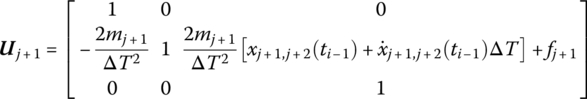
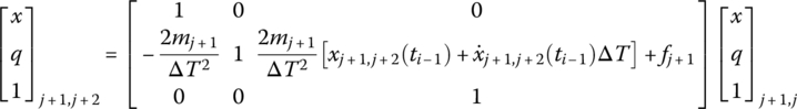
Equation (7.12) or Equation (7.13) is the transfer equation of a lumped mass, and Equation (7.14) is the transfer matrix of a lumped mass.
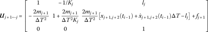
According to Equations (7.10) and (7.13), the transfer equation of the subsystem including the spring and lumped mass is
where ![]() is the transfer matrix of the subsystem:
is the transfer matrix of the subsystem:
that is
By simply assembling the transfer matrices of the subsystems, the overall transfer equation of the chain multibody system shown in Figure 7.1 is
The overall transfer matrix of the system is
Substituting the boundary conditions ![]() ,
, ![]() and the initial condition at time t0 into Equation (7.18), the unknown quantities of state vectors of the system boundary at time t1 can be obtained. For the chain multibody system shown in Figure 7.1,
and the initial condition at time t0 into Equation (7.18), the unknown quantities of state vectors of the system boundary at time t1 can be obtained. For the chain multibody system shown in Figure 7.1, ![]() and q0,1 at time t1 can be determined. The dynamics of all elements can be computed by using Equation (7.15), which can be considered as the initial condition for computing the dynamic response at time t2. The system dynamic response at an arbitrary time point is determined via the iterative method.
and q0,1 at time t1 can be determined. The dynamics of all elements can be computed by using Equation (7.15), which can be considered as the initial condition for computing the dynamic response at time t2. The system dynamic response at an arbitrary time point is determined via the iterative method.
For the model shown in Figure 7.1, we choose ![]() , with structure parameters and initial conditions according to Table 7.1. The computational results of motion by the transfer matrix method for linear multibody systems, the MSDTTMM and the Newton mechanics method, respectively, are shown in Figure 7.3. The solid line denotes the results computed by the Newton mechanics method, the symbol + denotes the results computed by the MSDTTMM and the symbol * denotes the results computed by the transfer matrix method for linear multibody systems. The results obtained by these three methods have good agreement and validate the proposed method.
, with structure parameters and initial conditions according to Table 7.1. The computational results of motion by the transfer matrix method for linear multibody systems, the MSDTTMM and the Newton mechanics method, respectively, are shown in Figure 7.3. The solid line denotes the results computed by the Newton mechanics method, the symbol + denotes the results computed by the MSDTTMM and the symbol * denotes the results computed by the transfer matrix method for linear multibody systems. The results obtained by these three methods have good agreement and validate the proposed method.
Table 7.1 Structure parameters and initial conditions
| Spring number | 1 | 3 | 5 | 7 | 9 |
| Stiffness K (N/m) | 1000 | 1000 | 1000 | 1000 | 1000 |
| Initial length l (m) | 0.1 | 0.1 | 0.1 | 0.1 | 0.1 |
| Lumped mass number | 2 | 4 | 6 | 8 | 10 |
| Mass m (kg) | 0.1 | 0.1 | 0.1 | 0.1 | 0.1 |
| External force f (N) | 100 | 0 | 0 | 0 | 0 |
| Initial displacement x0 (m) | 0.1 | 0.2 | 0.3 | 0.4 | 0.5 |
| Initial velocity |
0 | 0 | 0 | 0 | 0 |
Figure 7.3 Computational results by three methods.
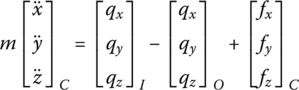
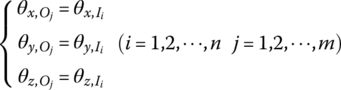
The state vector of a rigid body moving in space is defined as
where x, y, z, θx, θy and θz are the position coordinates of the connection point with respect to the inertial coordinate system and the corresponding rotation angles about the x, y and z axes. mx, my, ![]() , qx, qy and qz are the corresponding internal moments and forces in the same coordinate system.
, qx, qy and qz are the corresponding internal moments and forces in the same coordinate system.
The state vector of a rigid body moving in a plane is defined as
For the body element j with one input end and one output end, the transfer equation which relates the state vectors at its two points is
The transfer equation which relates the state vectors at the two points of a joint j is
where ![]() is the transfer matrix of element j.
is the transfer matrix of element j.
For a chain system composed of n elements, the overall transfer equation which relates the state vectors at the two points can be obtained by using Equations (7.22) and (7.23) repeatedly,
where
![]() is the overall transfer matrix of the system.
is the overall transfer matrix of the system.
Once the overall transfer matrix of the system is obtained, the boundary conditions of the system can be applied and the unknown quantities in the boundary state vectors can be computed. The state vectors of each element at time ti can be obtained using Equations (7.22) and (7.23) repeatedly and the system motion at time ti can be obtained. The entire procedure can be repeated for time ![]() and so on.
and so on.
7.3 Step‐by‐step Time Integration Method and Linearization
The linear MSTMM is established based on the fact that the internal forces at the same point are equal in magnitude, opposite in direction and act on different objects, resulting in a linear relationship between different points’ state vectors. For a nonlinear system, this linear relationship does not exist. Even for a linear time‐variant system, this linear relationship also does not exist. If we still want to use the transfer matrix method to study the dynamics of such a system, the linear relationship of state vectors between different points must be developed. Therefore, two questions must be answered: the first is whether physically nonlinear relations of state vectors involving transcendent functions or other complex relations can be expressed as linear forms; the second is how these complex relations can be linearly expressed to make the computation convergent and stable. The answers which come from modern science are affirmative. In fact, the increment transfer matrix method of a nonlinear time‐variant system was presented in Chapter 4 to compute the steady‐state response. For a time‐variant system, during the physical process of any computational time step size, if the time step size is small enough the relationship among many physical quantities can be approximately expressed by linear formulas. Modern numerical integral methods [222, 242, 247, 248] provide many linear forms to ensure computational convergence and stability. This section introduces these linearization methods of motion parameters and special functions that are based on step‐by‐step time integration methods.
7.3.1 Linearization of Velocity (Angular Velocity) and Acceleration (Angular Acceleration)
In dynamic equations of general elements, the unknown quantities include velocities (angular volocities), accelerations (angular accelerations), trigonometric functions and internal forces at connection points, as well as cross terms, high‐order terms and so on. For the free vibration of linear time‐invariant multibody systems, the state vectors satisfy the following relation:
where z is the physical coordinate and Z is the corresponding modal coordinate.
We can obtain
If the motion of a multibody system is aperiodic, Equation (7.26) does not exist. In order to develop the transfer matrix of an element, its dynamic equation must be linearized. Using numerical integral methods, velocity ![]() (angular velocity) and acceleration
(angular velocity) and acceleration ![]() (angular acceleration) can be expressed as linear functions of the position coordinate (angular coordinate), that is
(angular acceleration) can be expressed as linear functions of the position coordinate (angular coordinate), that is
where ![]() ,
, ![]() ,
, ![]() and
and ![]() at time ti are known functions with respect to time
at time ti are known functions with respect to time ![]() , and can be summarized as A, Bz, C and Dz.
, and can be summarized as A, Bz, C and Dz.
Based on the linearization of velocities, accelerations and other variables in a small time segment during time interval ![]() , the nonlinear dynamic equation at time ti can be expressed by linear formulas of the motion variables at time ti. The quantities above can be determined using the following methods.
, the nonlinear dynamic equation at time ti can be expressed by linear formulas of the motion variables at time ti. The quantities above can be determined using the following methods.
7.3.2 Step‐by‐step Time Integration Method
7.3.2.1 Forward–Euler Method
According to the Taylor expansion theorem, x(ti) can be approximately expressed as
From Equation (7.30), it follows that
Thus, the acceleration can be expressed approximately by the first‐order difference as ![]() from Equation (7.30), that is
from Equation (7.30), that is

By comparing Equations (7.30) and (7.31) with Equations (7.27) and (7.28), we obtain
7.3.2.2 Newmark‐β Method
Expanding the variable x(ti) at time ![]() by Taylor expansion theorem yields
by Taylor expansion theorem yields
Let
then

The velocity can be expressed by using Taylor expansion theorem as
Let
Substituting Equations (7.35) and (7.37) into Equation (7.36) yields
From Equations (7.35) and (7.38) we obtain
The Newmark‐β method originates from the trapezoid method, where only the first and second‐order derivatives of the Taylor series are adopted. The two parameters γ and β are used to compensate the contributions of the abandoned higher‐order quantities. If γ and β have different values, many formulas can be obtained. When ![]() and
and ![]() , this is the average acceleration method.
, this is the average acceleration method. ![]() leads to the constant acceleration method (center difference method), and
leads to the constant acceleration method (center difference method), and ![]() yields the linear acceleration method. It can be proved that if γ ≥ 1/2, β ≥ γ/2, and the formulas are unconditionally stable. If the value of β is increased, the computational precision will reduced, and if
yields the linear acceleration method. It can be proved that if γ ≥ 1/2, β ≥ γ/2, and the formulas are unconditionally stable. If the value of β is increased, the computational precision will reduced, and if ![]() , the computational precision is the highest, but the formula is conditionally stable. Newmark has pointed out that
, the computational precision is the highest, but the formula is conditionally stable. Newmark has pointed out that ![]() induces negative damping to a linear system, i.e. the vibration amplitude will be amplified in the integral computation. When
induces negative damping to a linear system, i.e. the vibration amplitude will be amplified in the integral computation. When ![]() , artificial damp will be introduced and finally induce reduction in the vibration amplitude. Generally, let γ ≥ 1/2. The most common choice is to let
, artificial damp will be introduced and finally induce reduction in the vibration amplitude. Generally, let γ ≥ 1/2. The most common choice is to let ![]() and then change β accordingly, so the method is called the Newmark‐β method. If
and then change β accordingly, so the method is called the Newmark‐β method. If ![]() and
and ![]() , this is the Forward–Euler method.
, this is the Forward–Euler method.
7.3.2.3 Wilson‐θ Method
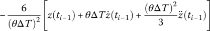
The Wilson‐θ method was developed on the basis of the linear acceleration assumption. The parameter θ ≥ 1 can be introduced in the time interval ![]() , assuming acceleration is linear with respect to time, as shown in Figure 7.4. A set of equations at time
, assuming acceleration is linear with respect to time, as shown in Figure 7.4. A set of equations at time ![]() , called predicted equations, is deduced first. Then the correction equations of displacement, velocity and acceleration at time
, called predicted equations, is deduced first. Then the correction equations of displacement, velocity and acceleration at time ![]() are deduced. When
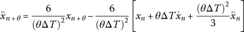
are deduced. When ![]() , this is the linear acceleration method. If τ is the time variable limited by 0 ≤ τ ≤ θΔT, the acceleration during this time interval can be written as
, this is the linear acceleration method. If τ is the time variable limited by 0 ≤ τ ≤ θΔT, the acceleration during this time interval can be written as ![]() , according to the assumption of linear acceleration. Later the acceleration can be integrated in [0, τ].
, according to the assumption of linear acceleration. Later the acceleration can be integrated in [0, τ].

Figure 7.4 Linear acceleration.
If ![]() , according to Equations (7.40) and (7.41), the velocity and displacement at time
, according to Equations (7.40) and (7.41), the velocity and displacement at time ![]() can be computed by the following two formulas
can be computed by the following two formulas
Combining Equations (7.42) and (7.43) yields
According to Equations (7.44) and (7.45), we obtain
7.3.2.4 Houbolt Method
The basic idea of the Houbolt method is that the velocity and acceleration at ![]() can be expressed approximately by the position coordinates of four points at previous times
can be expressed approximately by the position coordinates of four points at previous times ![]() , as shown in Figure 7.5. The relative coordinate
, as shown in Figure 7.5. The relative coordinate ![]() is introduced, and
is introduced, and ![]() ,
, ![]() , xn and
, xn and ![]() are the position coordinates corresponding to
are the position coordinates corresponding to ![]() , 1, 2 and 3, respectively. When 0 ≤ ζ ≤ 3, the position coordinate x(ζ) can be expressed approximately by the Lagrange interpolation polynomial:
, 1, 2 and 3, respectively. When 0 ≤ ζ ≤ 3, the position coordinate x(ζ) can be expressed approximately by the Lagrange interpolation polynomial:
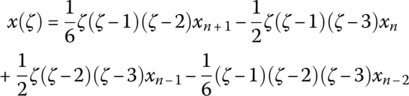
Figure 7.5 Houbolt method.
It is not difficult to figure out the rules of this interpolation polynomial: any individual term of this polynomial is the product of a position coordinate function and three terms of the four basic functions ζ, ![]() ,
, ![]() and
and ![]() . Its coefficients are obtained by the value of the function x(ζ) corresponding to each point. The first‐ and second‐order derivatives of x(ζ) are
. Its coefficients are obtained by the value of the function x(ζ) corresponding to each point. The first‐ and second‐order derivatives of x(ζ) are
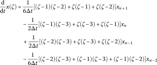
If ![]() , then
, then

Three previous time points are used in this linearization method, hence the first and second steps cannot be implemented in these formulations. The method can only be used if the information for three time points is known. This is the disadvantage of the multistep method. The two‐step and single‐step Houbolt methods are described here. Equation (7.50) yields
as
Adding Equations (7.53) and (7.54), then
Substituting Equation (7.55) into Equations (7.51) and (7.52), the linearization coefficients of the two‐step Houbolt method can be obtained:
As

then
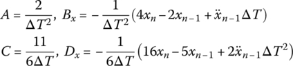
Therefore, the linearization coefficients of the one‐step Houbolt method become
In summary, the higher‐order Houbolt method can be constructed by a higher‐order Lagrange interpolation polynomial.
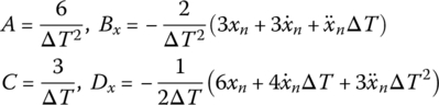
For different step‐by‐step time integration methods, different formulations of A, Bz, C and Dz can be obtained. Linearization coefficient formulations for different step‐by‐step time integration methods are shown in Table 7.2.
Table 7.2 Linearization coefficient for different step‐by‐step time integration methods
| Method | A | B z |
| TMM | 0 | |
| Forward–Euler | ||
| Newmark‐β | 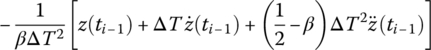 |
|
| Wilson‐θ |  |
 |
| Houbolt for i ≥ 3 | ||
| Houbolt for i = 2 | ||
| Houbolt for i = 1 | ||
| Method | C | Dz |
| TMM | 0 | 0 |
| Forward–Euler | ||
| Newmark‐β | ||
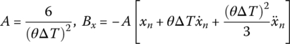
| Wilson‐θ | 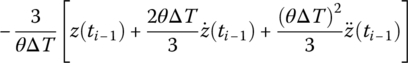 |
|
| Houbolt for i ≥ 3 | ||
| Houbolt for i = 2 | ||
| Houbolt for i = 1 |
Let the variable z represent a column matrix, such as the position coordinates ![]() or orientation angles
or orientation angles ![]() . At present, of the four linearization coefficients, A and C are irrespective of the state vector coefficient z, hence their expressions are invariant. Bz and Dz, however, should be rewritten as column matrices
. At present, of the four linearization coefficients, A and C are irrespective of the state vector coefficient z, hence their expressions are invariant. Bz and Dz, however, should be rewritten as column matrices ![]() and
and ![]() or
or ![]() and
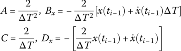
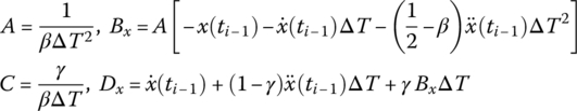
and ![]() , respectively. For example, in the Newmark‐β method
, respectively. For example, in the Newmark‐β method

7.3.3 Linearization of Nonlinear Functions
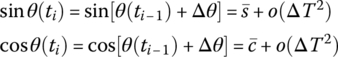
Correct to ΔT2, we expand the trigonometric functions at time ti as an explicit function of previous time ![]() by the Taylor expansion theorem, that is
by the Taylor expansion theorem, that is
where

In the geometric relationship from input end to output end, which includes trigonometric functions, the trigonometric functions can be linearized by the second‐order Taylor expansion, that is
For higher‐order terms in body dynamic equations, the second‐order terms can be expressed approximately as linear functions, that is
The linear expression of a third‐order function is

The above expansion formulations neglect the effect of terms that are higher than ΔT3 order. For higher‐order terms, their linearization expression can be obtained by using the same method.
The linearization expression of a general polynomial can be written as
where ![]() and
and ![]() at time ti are constants or functions of variables at previous times.
at time ti are constants or functions of variables at previous times.
Substituting differential for finite difference
yields
Hence

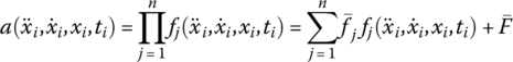
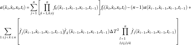
Linearization formulas of the trigonometric functions sin θ(ti), cos θ(ti) and higher‐order functions a(ti)b(ti) and a(ti)b(ti)c(ti) are used to derive the transfer matrices of elements. For convenience, all of these formulations are listed in Table 7.3.
Table 7.3 Linearization formulas of trigonometric functions and higher order functions
| Function | Linearization formulas |
| sin θ(ti) |  |
| cos θ(ti) |  |
| sin θ(ti) |  |
| cos θ(ti) |  |
| a(ti)b(ti) | |
| a(ti)b(ti)c(ti) |  |
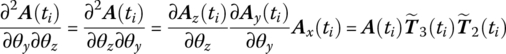
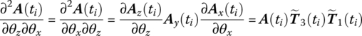
7.3.4 Linearization of Coordinate Transformation Matrices
The angular motion of a rigid body with respect to a fixed point can be realized by three rotations along three spatial fixed axes successively. The proof can be found in Appendix A.
A motion of a rigid body B relative to reference frame A is shown in Figure 7.6, where ![]() is any vector fixed in reference system A, and
is any vector fixed in reference system A, and ![]() is a vector fixed on rigid body B. Before B rotates relative to A,
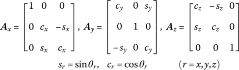
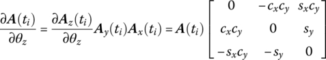
is a vector fixed on rigid body B. Before B rotates relative to A, ![]() . One fixed point’s 3 DOF rotation can be described by three angles which rotate in sequence around three arbitrary non‐coplanar axes. Herein we consider the angles θx, θy, θz that rotate in sequence around three spatial fixed axes in inertial coordinates. Therefore, the transform matrix, from the body‐fixed coordinate system to the inertial coordinate system, can be expressed by trigonometric functions of angles θx, θy, θz as follows:
. One fixed point’s 3 DOF rotation can be described by three angles which rotate in sequence around three arbitrary non‐coplanar axes. Herein we consider the angles θx, θy, θz that rotate in sequence around three spatial fixed axes in inertial coordinates. Therefore, the transform matrix, from the body‐fixed coordinate system to the inertial coordinate system, can be expressed by trigonometric functions of angles θx, θy, θz as follows:
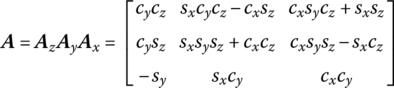

Figure 7.6 Simple rotation.
Where
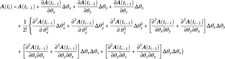
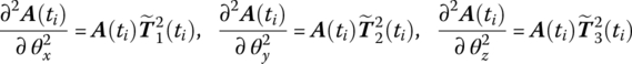
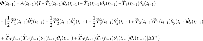
Using multiple Taylor expansion, for transform matrix ![]() at
at ![]() , keeping second‐order terms, we obtain
, keeping second‐order terms, we obtain
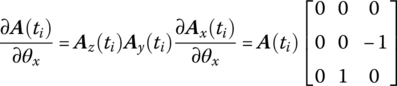
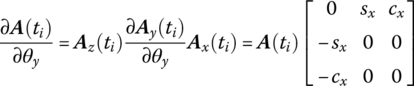
According to Equation (7.71)
Let
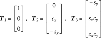
Then

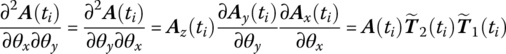
Similarly, it is easy to prove that
Combining Equations (7.71) and (7.78) yields
Let

Substituting Equations (7.78) to (7.82) into Equation (7.73) yields
where
7.4 Transfer Matrix of a Planar Rigid Body
A multi‐rigid‐body system is a system composed of several rigid bodies connected by all kinds of joints. Based on the MSDTTMM, once the transfer matrices of the elements are obtained, the multibody system dynamics can be computed and studied by simple programming matrix operations. It is important to point out that the transfer matrices of these elements remain the same for any multi‐rigid‐body systems and do not change with the structural variation of the multi‐rigid‐body system. The method provides flexibility in the modeling and computation of the dynamics of multibody systems with varying configuration, and this is one of the characteristics of the proposed method compared with any other method of multibody system dynamics. In this section, the dynamic equations of a rigid body are derived relative to the inertial coordinate system oxyz. The series uniform transfer equations and transfer matrices are deduced according to the input and output situations of all kinds of rigid bodies.
7.4.1 Planar Rigid Body with One Input End and One Output End
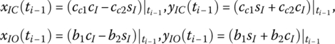
For the planar rigid body shown in Figure 7.7 the input end is I, the output end is O and the mass center is C. The inertial coordinate system is oxy and the body‐fixed coordinate system is O2x2y2 with origin I. In the coordinate system O2x2y2, the position coordinates of O are (b1, b2) and for the mass center C they are (cc1, cc2). The body‐fixed coordinate system is obtained by rotating o1x1y1 about the z2 axis with angle θ. Hence,
where
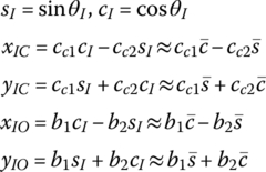
Figure 7.7 Rigid body moving in a plane with one input and one output end.
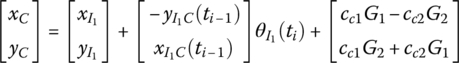
The external forces and moments acting on the rigid body are equivalent to the external forces and moments acting on the mass center of the rigid body. Therefore, we only consider the external forces and moments acting on the mass center of rigid bodies in the following analysis. The motion equation of the mass center is
where m is the mass of the rigid body and (xC, yC) are the position coordinates relative to the inertial coordinate system, while qx,I and qy,I are internal forces acting on the input end of the rigid body, and qx,O and qy,O are internal forces acting on the output end. fx,C and fy,C are external forces acting on the mass center of the rigid body.
According to the theorem of absolute angular momentum with respect to moving point I
The projection of Equation (7.92) on the inertial coordinate system can be written as
where ![]() is the absolute moment of momentum of the rigid body with respect to origin I of the body‐fixed coordinate system, and JI is the rotational inertia relative to point I.
is the absolute moment of momentum of the rigid body with respect to origin I of the body‐fixed coordinate system, and JI is the rotational inertia relative to point I. ![]() is the absolute angular velocity of the rigid body. rIC is the radius vector of the mass center C of the rigid body with respect to the point I, and aI is the absolute acceleration of point I.
is the absolute angular velocity of the rigid body. rIC is the radius vector of the mass center C of the rigid body with respect to the point I, and aI is the absolute acceleration of point I.
Linearizing Equations (7.88) and (7.89) using Equations (7.63) and (7.64) yields
Substituting Equations (7.86) and (7.87) into Equations (7.90) and (7.91), and linearizing using Equations (7.27), (7.63) and (7.64), we obtain
Substituting Equations (7.96) and (7.97) into Equation (7.93), and linearizing using Equation (7.27), we obtain
Combining Equations (7.85) and (7.95) to (7.98), the transfer equation of the rigid body moving in a plane with one input and one output end can be expressed as
The state vector is
and the transfer matrix is

where
7.4.2 Planar Rigid Body with Multiple Input and Multiple Output Ends
In this section, we derive the transfer equations and transfer matrices of rigid bodies with multiple input and multiple output ends, rigid bodies with one input end and multiple output ends, and rigid bodies with one output end and multiple input ends. For rigid bodies with multiple input and multiple output ends, we cannot obtain the main transfer equation from one point to another point. Only the matrix relation between input and output ends can be obtained.
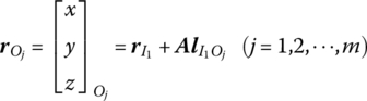
Figure 7.8 is the dynamic model of a rigid body moving in a plane. Assuming the input ends are ![]() and the output ends are
and the output ends are ![]() , the mass center is C. The inertial coordinate system is oxy. The coordinate system o1x1y1 is fixed on the first input end I1, and parallels the inertial coordinate system. The coordinate system O2x2y2 is the body‐fixed coordinate system and its origin is the same as o1x1y1. The position coordinates of the input and output ends in the coordinate system O2x2y2 are (a1,1, a2,1), (a1,2, a2,2),
, the mass center is C. The inertial coordinate system is oxy. The coordinate system o1x1y1 is fixed on the first input end I1, and parallels the inertial coordinate system. The coordinate system O2x2y2 is the body‐fixed coordinate system and its origin is the same as o1x1y1. The position coordinates of the input and output ends in the coordinate system O2x2y2 are (a1,1, a2,1), (a1,2, a2,2), ![]() and (b1,1, b2,1), (b1,2, b2,2)
and (b1,1, b2,1), (b1,2, b2,2) ![]() , respectively. The position coordinates of the mass center of the rigid body in the coordinate system O2x2y2 are (cc1, cc2).
, respectively. The position coordinates of the mass center of the rigid body in the coordinate system O2x2y2 are (cc1, cc2).
Figure 7.8 Rigid body with multiple input and multiple output ends moving in a plane.
Suppose we rotate o1x1y1 by angle θ to obtain body‐fixed coordinate O2x2y2. If ![]() , it is a one input end and one output end rigid body. When
, it is a one input end and one output end rigid body. When ![]() and
and ![]() , it is a rigid body with one input end and multiple output ends. When
, it is a rigid body with one input end and multiple output ends. When ![]() and
and ![]() , it is a rigid body with multiple input ends and one output end. When
, it is a rigid body with multiple input ends and one output end. When ![]() and
and ![]() , it is a rigid body with multiple input ends and multiple output ends.
, it is a rigid body with multiple input ends and multiple output ends.
Similarly to Equations (7.85) to (7.89), considering Equations (7.63) and (7.64) we obtain

where
(xC, yC) are the position coordinates of the mass center of a rigid body with respect to the inertial coordinate system. ![]() and
and ![]() are the position coordinates of the input end Ij and the output end Oj in the inertial coordinate system.
are the position coordinates of the input end Ij and the output end Oj in the inertial coordinate system.
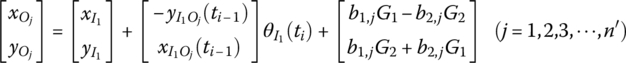
In the following analysis, we only consider the external force and external moment acting on the mass center of the rigid body. According to the dynamic equation of the mass center of a rigid body
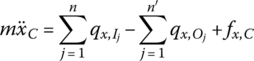
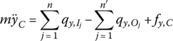
where m is the mass of the rigid body, ![]() and
and ![]() are the internal forces acting on the input end of the rigid body,
are the internal forces acting on the input end of the rigid body, ![]() and
and ![]() are the internal forces acting on the output end of the rigid body, and fx,C and fy,C are the external forces acting on the mass center of the rigid body.
are the internal forces acting on the output end of the rigid body, and fx,C and fy,C are the external forces acting on the mass center of the rigid body.
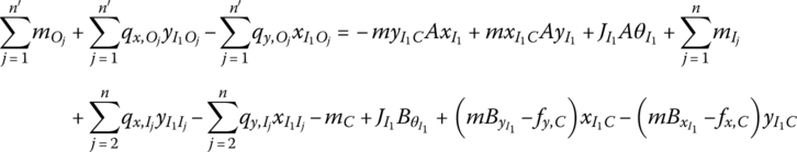
Based on the theorem of the absolute angular momentum on the moving momentum center, which is the first input end I1, we obtain
The projection of Equation (7.117) on the inertial coordinate system can be written as
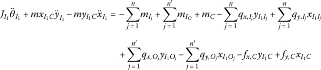
Substituting Equations (7.27), (7.106), (7.63) and (7.64) into Equations (7.115) and (7.116) yields


Substituting Equations (7.27), (7.119) and (7.120) into Equation (7.118) yields
Equations (7.107) and (7.104) can be written in matrix form
where
Equations (7.105) and (7.108) can be written in matrix form
where
Equations (7.119) to (7.121) can be written in matrix form
where
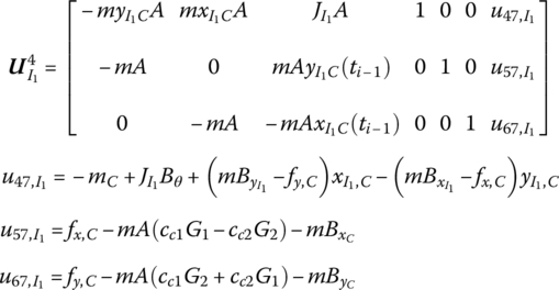
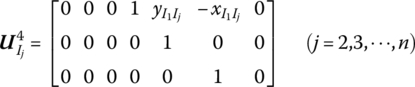

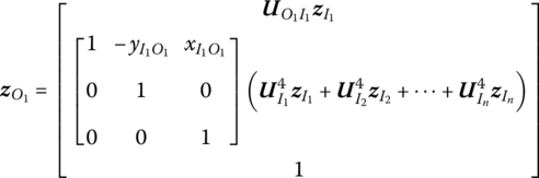
The state vector of the rigid body with multiple input ends and multiple output ends can be defined as
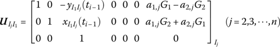
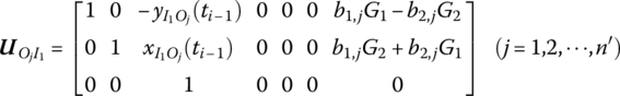
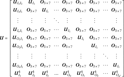
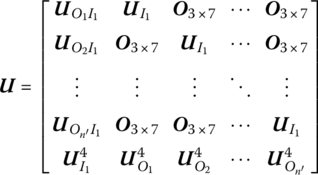
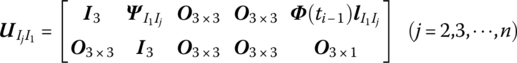
According to Equations (7.122), (7.125) and (7.127), the transfer equation of the rigid body with multiple input ends and multiple output ends is
The transfer matrix is
Similarly, the transfer equations and transfer matrices of the rigid body with multiple input ends and one output end, and the rigid body with one input end and multiple output ends can be obtained, which are provided in the following sections without the detailed deduction procedures.
7.4.2.1 Transfer Equation and Transfer Matrix of a Rigid Body moving in a Plane with Multiple Input Ends and One Output End
State vector
Transfer equation
Transfer matrix
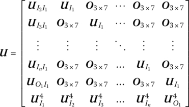
All submatrices are the same as those in Equation (7.133).
For computation convenience, ![]() can be expressed by
can be expressed by ![]() as
as
7.4.2.2 Transfer Equation and Transfer Matrix of a Rigid Body Moving in a Plane with One Input End and Multiple Output Ends
State vector
Transfer equation
Transfer matrix
All submatrices are the same as those in Equation (7.133).
For computation convenience, ![]() can be expressed by
can be expressed by ![]() as
as
where
7.5 Transfer Matrices of Spatial Rigid Bodies
In this book, the spatial motion of a multibody system is studied in the inertial coordinate system using three spatial angles about the x–y–z axis defined in reference [9], which is very convenient for the transformation of state vectors.
7.5.1 Spatial Rigid Body with One Input End and One Output End
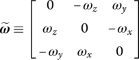
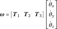
The column matrix of the angular velocity of a rigid body with respect to the inertial coordinate system in the body‐fixed coordinate system of a rigid body is
and its skew symmetric matrix is
The first‐order derivative with respect to time of transformation matrix ![]() defined in Equation (7.71) is
defined in Equation (7.71) is

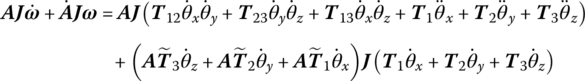
The dynamics equation and transfer matrix are deduced using the three spatial axis angles about x–y–z, that is

where

It can be proved that
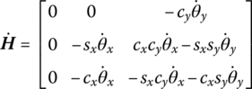
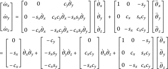
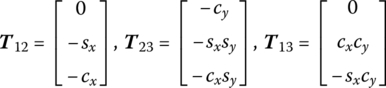
The first‐order derivative with respect to the time of the angular velocity ω of the rigid body in the inertial coordinate system is
The time derivative of Equation (7.144) is
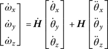
where
For a rigid body moving in space, as shown in Figure 7.9, the column vectors of the rotation angle and positions are defined as ![]() and
and ![]() , respectively. For the input end and output end
, respectively. For the input end and output end
where ![]() is the coordinate transformation matrix from O2x2y2z2 to o1x1y1z1.
is the coordinate transformation matrix from O2x2y2z2 to o1x1y1z1.
Figure 7.9 Rigid body moving in space.
If only the external force and moment acting on the mass center of the rigid body are considered, according to the motion equation of the mass center
where m is the mass of the rigid body and ![]() is the radius vector of the mass center of the rigid body with respect to the origin of the inertial coordinate system.
is the radius vector of the mass center of the rigid body with respect to the origin of the inertial coordinate system. ![]() is the internal force acting on the input end of the rigid body,
is the internal force acting on the input end of the rigid body, ![]() is the internal force acting on the output end of rigid body and
is the internal force acting on the output end of rigid body and ![]() is the external force acting on the mass center of the rigid body.
is the external force acting on the mass center of the rigid body.
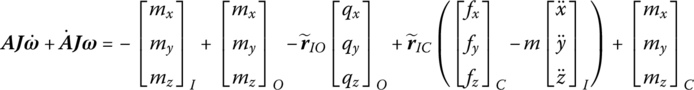
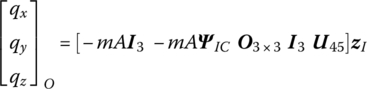
The projection of Equation (7.152) on the inertial coordinate system can be written as
where ![]() is the coordinate column matrix of the mass center of the rigid body with respect to the inertial coordinate system:
is the coordinate column matrix of the mass center of the rigid body with respect to the inertial coordinate system:
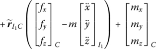
According to the theorem of absolute angular momentum to the moving momentum center, we obtain
The projection of Equation (7.155) on the inertial coordinate system can be written as
where ![]() ,
, ![]() and
and ![]() is the absolute moment of momentum of the rigid body with respect to point I.
is the absolute moment of momentum of the rigid body with respect to point I. ![]() and
and ![]() are the internal moments acting on points I and O, respectively,
are the internal moments acting on points I and O, respectively, ![]() is the internal forces acting on point O,
is the internal forces acting on point O, ![]() is the external moment acting on the mass center of the rigid body,
is the external moment acting on the mass center of the rigid body, ![]() is the acceleration of the point I and
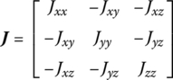
is the acceleration of the point I and ![]() is the inertia matrix of the rigid body with respect to point I in the body‐fixed coordinate system.
is the inertia matrix of the rigid body with respect to point I in the body‐fixed coordinate system.
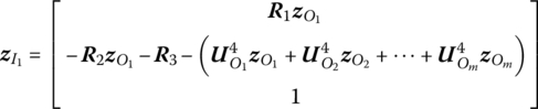
The transfer matrix is now derived. Substituting Equation (7.83) into Equation (7.151), we obtain

where
![]() ,
, ![]() and
and ![]() can be obtained by Equations (7.84), (7.77) and (7.20), respectively.
can be obtained by Equations (7.84), (7.77) and (7.20), respectively.
Equation (7.150) can be written as
Linearizing the left‐hand terms of Equation (7.153) yields
Replacing the subscript O in Equation (7.158) by C, we obtain
Substituting Equation (7.161) into Equation (7.160) yields
where
The coordinate column matrix of angular acceleration in the body‐fixed coordinate system can be obtained, that is
Let
then the coordinate column matrix of angular acceleration in the body‐fixed coordinate system can be rewritten as
Combining Equations (7.144) and (7.77) yields
According to Equations (7.145), (7.164) and (7.165)
Let
then
where
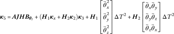

Substituting Equations (7.27) and (7.169) into Equation (7.156) yields

where
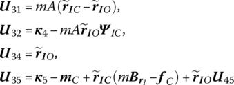
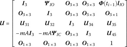
Combining Equations (7.158), (7.159), (7.162) and (7.172), the transfer equation of a rigid body moving in space with one input end and one output end can be obtained:
The transfer matrix is
7.5.2 Spatial Rigid Body with Multiple Input and Multiple Output Ends
7.5.2.1 Transfer Equation and Transfer Matrix of a Rigid Body moving in Space with Multiple Input and Multiple Output Ends
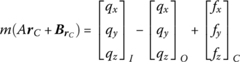
The dynamics model of a rigid body moving in space with multiple input and multiple output ends is shown in Figure 7.10. ![]() are input ends,
are input ends, ![]() are output ends and C is the mass center of the rigid body. The inertial coordinate system is oxyz. The origin of the coordinate system o1x1y1z1 is the first input end I1 of the rigid body, which is parallel to the inertial coordinate system. The origin of the body‐fixed coordinate system O2x2y2z2 is the same as the coordinate system o1x1y1z1. The coordinates of the input and output ends in the body‐fixed coordinate system O2x2y2z2 are (a1,j, a2,j, a3,j) and (b1,j, b2,j, b3,j), respectively, and the coordinates of the mass center are (cc1, cc2, cc3). Then;
are output ends and C is the mass center of the rigid body. The inertial coordinate system is oxyz. The origin of the coordinate system o1x1y1z1 is the first input end I1 of the rigid body, which is parallel to the inertial coordinate system. The origin of the body‐fixed coordinate system O2x2y2z2 is the same as the coordinate system o1x1y1z1. The coordinates of the input and output ends in the body‐fixed coordinate system O2x2y2z2 are (a1,j, a2,j, a3,j) and (b1,j, b2,j, b3,j), respectively, and the coordinates of the mass center are (cc1, cc2, cc3). Then;
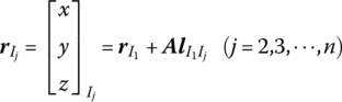
where ![]() and
and ![]() are the coordinates column matrices of the input and output ends in the inertial coordinate system, rC is the vector of the mass center relative to the origin of the inertial coordinate system,
are the coordinates column matrices of the input and output ends in the inertial coordinate system, rC is the vector of the mass center relative to the origin of the inertial coordinate system, ![]() are the coordinates column matrix of the mass center of the rigid body in the inertial coordinate system and A is the transformation matrix from the coordinate system O2x2y2z2 to o1x1y1z1.
are the coordinates column matrix of the mass center of the rigid body in the inertial coordinate system and A is the transformation matrix from the coordinate system O2x2y2z2 to o1x1y1z1.
Figure 7.10 Rigid body moving in space with multiple input and multiple output ends.
Linearizing Equations (7.175) and (7.176) yields
where

Linearizing Equations (7.175) and (7.177) yields
where
According to the dynamic equation of the mass center of the rigid body, we obtain
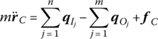
Projecting Equation (7.181) into the inertial coordinate system yields
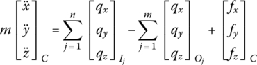
where m is the mass of the rigid body. ![]() are the internal forces at the input ends and
are the internal forces at the input ends and ![]() are the internal forces at the output ends. fC is the external force acting on the rigid body mass center.
are the internal forces at the output ends. fC is the external force acting on the rigid body mass center.
According to the theorem of absolute angular momentum to the moving momentum center, the dynamics equation of a rigid body with multiple input and multiple output ends can be written as

Projecting Equation (7.183) into the inertial coordinate system yields
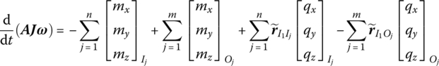
where

Linearizing Equations (7.182) and (7.184) yields
where
The state vector of a rigid body with multiple input ends and multiple output ends can be defined as
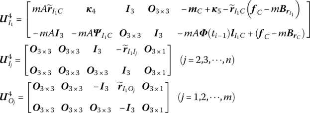
Combining Equations (7.179), (7.180) and (7.185), the transfer equation of a rigid body with multiple input ends and multiple output ends can be obtained
The transfer matrix is

In a similar manner, the transfer equations and transfer matrices of a rigid body with multiple input ends and one output end, and a rigid body with one input end and multiple output ends can be found. The results are given in the following sections.
7.5.2.2 Transfer Matrix of a Rigid Body with Multiple Input Ends and One Output End
State vector
Transfer equation
Transfer matrix
All submatrices are the same as those in Equation (7.188).
For ease of calculation, ![]() can be expressed by
can be expressed by ![]() , hence
, hence
7.5.2.3 Transfer Matrix of a Rigid Body with One Input End and Multiple Output Ends
State vector
Transfer equation
Transfer matrix

All submatrices are the same as those in Equation (7.188).
For ease of calculation, ![]() can be expressed by
can be expressed by ![]() , hence
, hence
where
7.6 Transfer Matrices of Planar Hinges
The interaction (such as damper, spring, driven constraint or motion and contact) between different bodies can be regarded as a force element in the ordinary dynamics methods of multibody systems. However, in MSDTTMM, the interactions between different bodies can be regarded as hinges, and that makes dynamic modeling more convenient and flexible.
7.6.1 Elastic Hinges
Here, the elastic hinge consists of linear (or nonlinear) spring hinges and linear (or nonlinear) rotary spring hinges. Figures 7.11 and 7.12 illustrate the models for linear spring and nonlinear spring forces, respectively.
Figure 7.11 Linear spring force model.
Figure 7.12 Nonlinear spring force model.
Ignore the mass and the initial length of the spring and assume
where ![]() is the change in length of a spring in the xy plane. O denotes the output end and I denotes the input end.
is the change in length of a spring in the xy plane. O denotes the output end and I denotes the input end. ![]() is the spring force, and K1 and K2 are the stiffness coefficients of a nonlinear spring.
is the spring force, and K1 and K2 are the stiffness coefficients of a nonlinear spring.
Projection of Equation (7.197) into the ox and oy directions results in
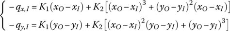
Substituting Equation (7.66) into Equation (7.198) yields
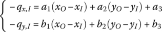
where
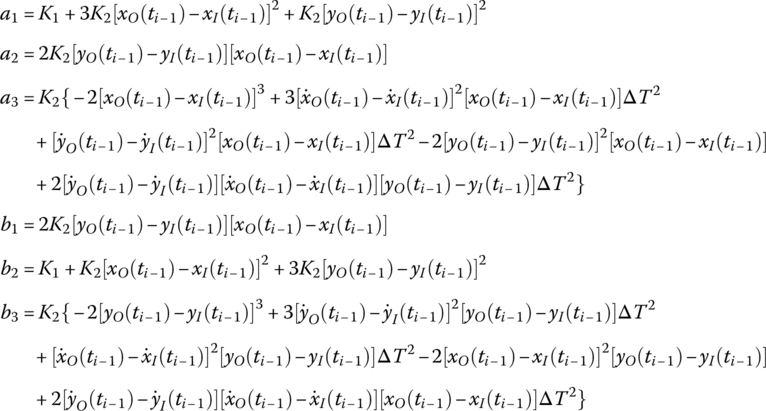
According to Equation (7.199), we obtain
where

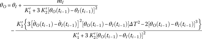
The moment of a nonlinear rotary spring is
where ![]() and
and ![]() are the stiffness coefficients.
are the stiffness coefficients.
Similarly, linearizing Equation (7.202), we obtain
For linear spring and rotary spring hinges whose masses are neglected, we obtain
Rewriting Equations (7.200), (7.201) and (7.203) to (7.206) in terms of matrices, the transfer equation of a spring moving in a plane is
The state vector is
and the transfer matrix is

where

For a linear spring, that is, ![]() , the transfer matrix can be derived from Equation (7.208) as
, the transfer matrix can be derived from Equation (7.208) as

7.6.2 Damper Hinges
For a viscous damper, the viscous damped forces and damped moment are
where Cd and ![]() are the damping coefficients of translational dampers and rotary dampers, respectively.
are the damping coefficients of translational dampers and rotary dampers, respectively.
Linearizing Equation (7.210), we obtain
From Equations (7.211) to (7.213), the transfer equation of a viscous damper hinge moving in a plane is
The state vector is
and the transfer matrix is
where
7.6.3 Smooth Hinges
For the smooth hinge shown in Figure 7.13, at the two ends the position coordinates and internal forces are equal and the internal torques are constant zero:
Figure 7.13 Model of a smooth hinge.
The numbers of inboard and outboard bodies of the smooth hinge j are ![]() and
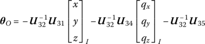
and ![]() , respectively. In the following, the rotation angle θO of the outboard body
, respectively. In the following, the rotation angle θO of the outboard body ![]() of a smooth hinge is discussed for two cases.
of a smooth hinge is discussed for two cases.
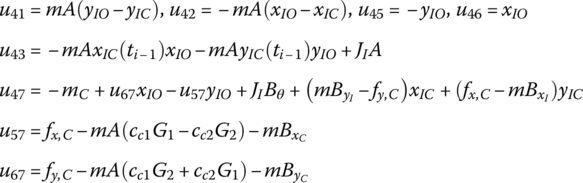
7.6.3.1 Smooth Hinge whose Outboard is a Rigid Body and with Internal Torques at the Output End of Zero
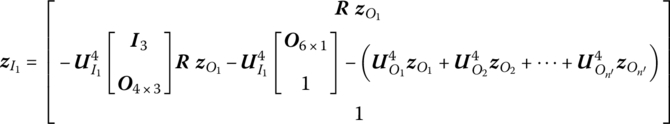
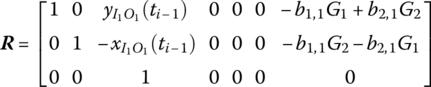
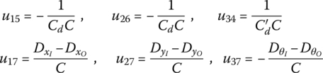
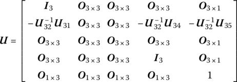
If another point of the outboard rigid body is also connected to a smooth hinge or a free boundary, then we can obtain the transfer equation of the outboard rigid body of the smooth hinge
where u41, u42, u43, u45, u46 and u47 are elements of the transfer matrix of the outboard rigid body.
Substituting Equation (7.216) into Equation (7.217) yields
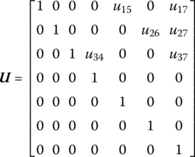
Combining Equations (7.216) and (7.218), and referring to the state vectors defined by Equation (7.21), we obtain the transfer equation of the smooth hinge whose outboard is a rigid body and whose internal torques of the output end are zero, namely
The transfer matrix is
In Equation (7.219), the element u4,4 could also be written as “1”. However, if we set ![]() , the computational precision will be improved. According to the above derivation, if the internal moments of the outboard body at the two ends of the smooth hinge are equal to zero, the above transfer equation and transfer matrix are valid.
, the computational precision will be improved. According to the above derivation, if the internal moments of the outboard body at the two ends of the smooth hinge are equal to zero, the above transfer equation and transfer matrix are valid.
7.6.3.2 Smooth Hinge whose Outboard is a Rigid Body and with Nonzero Internal Torques at the Output End
The output end of the outboard rigid body of a smooth hinge is connected to an elastic hinge or a damper hinge, as shown in Figure 7.14. Among the outboard elements of the smooth hinge, if there is such an element whose internal moment is always zero or with free boundaries, then the transfer equation of this smooth hinge can be deduced in the following way. The transfer equation of the subsystem from the smooth hinge to the hinge whose internal moment is zero can be derived as
Figure 7.14 Model of a multibody system.
The transfer matrix is
where ![]() are the transfer matrices of the outboard elements of the smooth hinge.
are the transfer matrices of the outboard elements of the smooth hinge.
Because the internal moments in the state vectors ![]() of the output end of the smooth hinge and the state vector
of the output end of the smooth hinge and the state vector ![]() of the output end of the subsystem are all equal to zero, we can obtain the transfer equation and transfer matrix of the smooth hinge which are similar to the form of Equation (7.219), where,
of the output end of the subsystem are all equal to zero, we can obtain the transfer equation and transfer matrix of the smooth hinge which are similar to the form of Equation (7.219), where, ![]() are elements of the transfer matrix
are elements of the transfer matrix ![]() .
.
7.7 Transfer Matrices of Spatial Hinges
7.7.1 Elastic and Damper Hinges
The elastic damper hinge is composed of a linear spring hinge with a parallel connected damper, combining a rotary spring with a parallel connected damper. As shown in Figure 7.15, element ![]() is the elastic joint and damper, whose inboard body and outboard body are rigid bodies j and
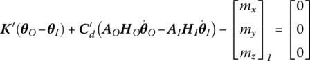
is the elastic joint and damper, whose inboard body and outboard body are rigid bodies j and ![]() , respectively. According to the force equilibrium at points O and I, we obtain
, respectively. According to the force equilibrium at points O and I, we obtain

where
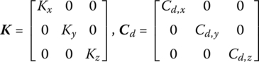
Figure 7.15 Elastic and damper hinges.
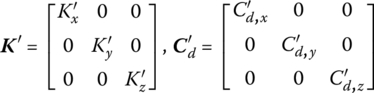
Kx, Ky and Kz are the stiffness coefficients of the spring along the three axes of the inertial coordinate system, respectively, and Cd,x, Cd,y and Cd,z are the damper coefficients of the translation damper in the three axes of the inertial coordinate system, respectively.
Linearizing the velocity item yields
where
and ![]() is defined as in Equation (7.20).
is defined as in Equation (7.20).
For the rotational spring and damper we obtain
where
The definitions of ![]() and
and ![]() can be seen in Equations (7.71) and (7.144).
can be seen in Equations (7.71) and (7.144). ![]() ,
, ![]() and
and ![]() are the stiffness coefficients of the rotational spring along the three axes of the inertial system, respectively, and
are the stiffness coefficients of the rotational spring along the three axes of the inertial system, respectively, and ![]() ,
, ![]() and
and ![]() are the damper coefficients of the rotational damper about the three axes of the inertial system, respectively.
are the damper coefficients of the rotational damper about the three axes of the inertial system, respectively.
Linearizing Equation (7.223), we obtain
where
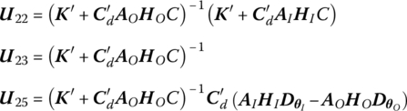
The transfer equation of the spring joint and damper moving in space can be written as
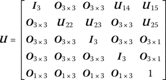
The transfer matrix is
7.7.2 Smooth Ball‐and‐socket Hinge whose Outboard is a Rigid Body and with Internal Torques at the Output End of Zero
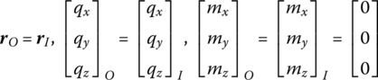
For a smooth ball‐and‐socket hinge, using a similar method as for the smooth hinge moving in a plane, its mass and size can be neglected. The position coordinates and internal forces are equal and the internal moments are constant zero at its two ends, that is
The ![]() and
and ![]() denote the numbers of the inboard body and outboard body of the smooth ball‐and‐socket hinge j. For a smooth ball‐and‐socket hinge, if its outboard is a rigid body and the internal moment of the output end of this rigid body is zero, then by using the transfer equation of the outboard body of the smooth ball‐and‐socket joint, we obtain:
denote the numbers of the inboard body and outboard body of the smooth ball‐and‐socket hinge j. For a smooth ball‐and‐socket hinge, if its outboard is a rigid body and the internal moment of the output end of this rigid body is zero, then by using the transfer equation of the outboard body of the smooth ball‐and‐socket joint, we obtain:
where ![]() ,
, ![]() ,
, ![]() and
and ![]() are submatrices of the transfer matrix of the smooth ball‐and‐socket joint’s outboard body.
are submatrices of the transfer matrix of the smooth ball‐and‐socket joint’s outboard body. ![]() is defined in Equation (7.20).
is defined in Equation (7.20).
Substituting Equation (7.226) into Equation (7.227) yields
Combining Equations (7.226) and (7.228), the state vectors are derived by Equation (7.20), and the transfer equation of the smooth ball‐and‐socket joint can be derived as
The transfer matrix is
7.7.3 Smooth Ball‐and‐socket Hinge whose Outboard is a Rigid Body and with Nonzero Internal Torques at the Output End
If the internal moment of the output end of the outboard rigid body of the smooth ball‐and‐socket joint is nonzero, the transfer matrix and transfer equation of smooth ball‐and‐socket joint can be obtained by using the same method as in section 7.6.3. The form is the same as in Equation (7.220).
7.8 Algorithm of the Discrete Time Transfer Matrix Method for Multibody Systems
The algorithm to compute multi‐rigid‐body system dynamics using MSDTTMM is as follows:
- Determine the initial conditions and the boundary conditions of the system and set i = 1.
- Compute the coefficients A, Bz (or Bz), C, Dz (or Dz),
 ,
,  ,
,  ,
,  ,
,  ,
,  ,
,  etc. at time ti for each connecting element by the linearization method, and determine the initial conditions
  ,
,  and
and  at time ti as well as the system parameters.
 - Formulate the transfer matrix for each subsystem and the overall transfer matrix at time ti, respectively.
- Apply the boundary conditions and the overall transfer equation to compute the unknown quantities in the boundary state vectors at time ti.
- By using the transfer equations of each element, compute the state vectors of each element at time ti.
- Use the state vectors at time ti to compute the first‐ and second‐order derivatives of the position coordinates and rotation angles with respect to time.
- Let
 , use the computational result of the last step as the initial conditions, and return to step (2). This procedure is repeated until the final time step is accomplished.
7.9 Numerical Examples of Multibody System Dynamics
7.9.1 Chain Multibody System Dynamics
For the chain multibody system shown in Figure 7.16, the transfer equations of hinge element j and body element ![]() are
are
where ![]() are the transfer matrices of hinge j and body
are the transfer matrices of hinge j and body ![]() .
.

Figure 7.16 Chain multibody system.
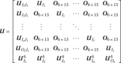
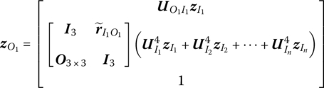
The overall transfer equation of the system can be assembled by only using the transfer matrices of these elements, that is
where the overall transfer matrix is
For a chain multibody system, the overall transfer matrix of the system can be obtained by successive multiplication of the transfer matrices of the elements. The order of the overall transfer matrix of the system is equal to the highest order of the transfer matrices of the elements, and it does not change as the number of DOFs in the system increases. For a chain multi‐rigid‐body system moving in a plane, the highest order of the transfer matrix is (7 × 7), while for a chain multi‐rigid‐body system moving in space, the highest order is (13 × 13).
Substituting the boundary conditions into the overall transfer equation of the system, the unknown quantities in the state vectors of the system boundaries can be computed. The state vectors and the motion quantities of each element at time ti can be computed by repeatedly using the corresponding transfer equations of elements. The quantities of velocity, angular velocity, acceleration and angular acceleration at time ti can be obtained. Repeating the entire procedure can allow the system motion to be obtained.