
1
Introduction
1.1 The Status of the Multibody System Dynamics Method
A multibody system (MS) is a system composed of many bodies, including rigid bodies, flexible bodies, lumped mass, etc., connected in various ways. The physical concept of an MS is ancient and unambiguous. In the construction of national defense and the economy, such as weaponry, shipping, aeronautics, astronautics, communications and mechanisms, many models of practice engineering, such as tanks, ships and warships, aircraft, carrier rockets, vehicles, robots, machine tools etc., can be regarded as MSs composed of rigid bodies, flexible bodies and lumped masses connected with various hinges [1–12].
In the 1950s to the 1960s, the concept of a multibody was either a multi‐rigid‐body or a multi‐flexible‐solid, therefore two totally different subjects, multi‐rigid‐body system dynamics (MRSD) [7, 9, 11] and the finite element method (FEM) [13], respectively, were developed almost independently. The infinite element method [14], presented in the mid‐1970s, perhaps is a little supplement for the FEM. The basis of MRSD is the ancient dynamics and variation principle. The research objects of multibody system dynamics (MSD) [6, 8, 12] are a rigid body and flexible solid, which includes both the research objects of MRSD and the FEM. Since the dynamics equation of a rigid body rotating around a fixed point was established by Euler in 1765, rigid body theory has had more than 200 years of history and is very distinct. In the classical theory of rigid body dynamics developed since 1960s, only a few systems with more than two bodies, such as double pendulums and gyroscopes, have been studied. Complex multi‐rigid‐body systems (MRSs) composed of many rigid bodies moving on a large scale connected with various hinges has not been studied enough in flexible solid dynamics and the FEM. It is known that the model of the MRS is not a good enough mechanics model for practical problems. For example, a slender manipulator should not be modeled as a rigid body, and a slender tube of a rocket launcher and gun should also not be modeled as a rigid body in the study of launch dynamics. It is necessary to include the flexible body for further study of MSD. The multi‐rigid‐flexible‐body system (MRFS) has become the main research direction in MSD and the main dynamics model for many engineering mechanism systems. The hybrid algorithm of the MRS and the FEM [10], developed by Professor Peter Eberhard of the University of Stuttgart and Dr. Bin Hu of the Mercedes‐Benz Company in 2003, combines the highlight of multi‐rigid‐body dynamics and the FEM, and has the features of high computation efficiency and high computation accuracy when computing the dynamics of a flexible body with large motion using this method. It is one of the recommended advanced methods of contact dynamics.
Since the discovery of Hooke’s law in 1660 to now, the solid theory has had more than 300 years of history and is very distinct. Beginning in the 1950s, the solid theory and the deformation of elastic solids have progressed to finite deformation nonlinear elastic theory by elastic mechanics based on a formulation system [15]. However, the rigid body and its large motion have not been involved in elastic mechanics. It is necessary to have a unanimous opinion for the concept of solid rotation. The rotation of a rigid body is a characteristic quantity of global body movement of the rigid body and is independent of the origin of its translation coordinate system. How can we model the rotation of an elastic body, such as an elastic manipulator that has one end fixed on a rotational axis? The rotation of a point fixed on a deformable solid is used to describe the rotational displacement of the adjacent region of such a point, rather than to specify the characteristic quantity of the global movement of the whole solid. It is therefore necessary to include the rigid body in the further study of solid dynamics.
Multi‐flexible‐body system dynamics (MFSD) [6, 8, 12] is the current research focus in MSD. It differs not only from MRSD, but also from classical solid dynamics. Its main characteristic is coupling between the deformation and the global rigid motion of the body; the consideration of the flexible effect in the dynamics equations of MSs plays a key role. There are usually two methods of treating a flexible body. One is to model a flexible body using many rigid bodies connected by springs and dampers, and the other is to establish the dynamics equation of the flexible body directly and describe its deformation with the FEM, the modal synthesis method or the hypothesis modal shape method. The “multi‐flexible‐body system” emphasizes the two aspects of multibody and flexibility. Multibody means that MFSD is the natural extension of MRSD, as usually there is large motion among bodies. Flexibility of body means that MFSD is the natural extension of solid dynamics; it makes the number of degrees of freedom (DOF) of the flexible body increase greatly and the relations between kinematics and dynamics more complex. The centrifugal forces and Coriolis forces acting on a body, caused by its large motion, affect its deformation and the deformation conversely affects the composite motion of the body. The coupling effect between large motion and deformation of the body is the core of MFSD.
Along with the development needs of engineering technology, many methods of MSD, such as the Wittenburg method [7], the Schiehlen method [6] and the Kane method [9] etc. [16–28], have been put forward and improved creatively by scholars and experts in the last 50 years. These methods provided effective computation means for various MSD, and greatly boosted the development of modern engineering technology. Based on the FEM and the boundary element method (BEM), the programming of structure dynamics analysis was realized. These theories provided powerful tools for complex structure dynamics. Various computational programs, such as SAP, NASTRAN and ANSYS, have been developed. Although the various methods of MSD have different styles, they all have the following two characteristics. First, it is vital to establish the global dynamic equation of the system, which is the most wonderful part of each MSD, marked by individual features, and is the most baffling part for ordinary technicians. Second, the order of the system matrix of the global dynamic equation of the system is not less than the number of degrees of freedom of the system and is very high for a complex system, resulting in a big problem regarding its computational scale. These two problems in the FEM and ordinary methods of MSD have been given great attention. First, it is not convenient to compute the vibration characteristics of complex MRFSs with a high stiffness gradient. Second, it is difficult to exactly analyze the system dynamic response because of a lack of eigenvector orthogonality of the general complex MRFS. The following academic and practical problems have been given great attention by dynamicists and engineers around the world [29–33]: avoiding the computation singularity caused by the computation ill‐condition of a structure with a high stiffness gradient, finding the eigenvector orthogonality of general MRFS coupled with rigid bodies and flexible bodies, searching for efficient computational methods of MRFSD with high programmability, thinking of and designing dynamic launch system performance from the point of launch system dynamics.
To solve these problems can we develop a new way that is completely different from the study styles and features of ordinary MSD as follows: without the global dynamic equation of system, with a small computational scale and highly programmable? Motivated by the idea of the transfer between state vectors used in the classical transfer matrix method (TMM) [34–40], a totally new method with these features, the transfer matrix method for multibody systems (MSTMM) [3–5, 41–86], has been developed by the authors. The MSTMM applies to a linear multibody system, as well as a general multibody system, to compute their dynamic responses. In particular, the vibration characteristics of a linear multibody system can be solved by using the MSTMM. The technologies of dynamic design [87–121] are developed for improving the launch precision of launch systems, reducing the ammunition consumption of launch system tests, diagnosing faults, etc. These solved the important engineering problems of a series of national high‐technique subjects, such as self‐propelled artillery, shipboard launch systems, multiple launch rocket systems (MLRSs), missile sealift systems with ocean wave compensation, application of the strap‐down inertial measurement unit of the gyroscope, and accelerometers with high precision. These injected new energy into and provided completely new methods for the development of launch dynamics and flight dynamics [122–200].
1.2 The Transfer Matrix Method and the Finite Element Method
The classical TMM was developed in the 1920s to analyze the vibration of one‐dimensional linear systems with an elastic construct (see references [36–38]). Holzer (1921) first used the parameter method, named the Holzer method, to solve torsional vibration for shafts with multiple discs [201]. Myklestad (1944) used a similar method to determine the bend vibration modes of beams [202]. Proh (1945) improved the Holzer method, resulting in the so‐called Myklestad method, to solve the transverse vibration of shafts [203]. With the development of computer and matrix operations, the Myklestad method was worked up to create the TMM. Thomson (1950) used the TMM to structure vibration of the general linear system [204]. Pestel (1963) published the first TMM book [36], Matrix Method in Elastomechanics. Many transfer matrices of elastic mechanics elements are given in this book. Rubin (1964) put forward the general method for the transfer matrix and the relationship between the transfer matrix and the frequency response matrix [205]. The TMM was used by many scholars and engineers, such as Targoff [206], Lin [207], Mercer [208], Lin [209], Mead [210, 211], Henderson [212], McDaniel [213, 214] and Murthy [215–217], to solve static and dynamic engineering problems for beams, beam‐type multiple structures, skin‐stringer panels, rib–skin structures, curved multi‐span structures, cylindrical shells, stiffened rings, etc. Horner (1978) presented the Riccati TMM [218] to solve the numerical stability of boundary value problems. Huolang Fang (1990) used Fourier–Laplace transformation to derive the transfer matrix of three‐dimensional viscoelastic groundsill floors with invariant mass density under harmonic loads and solve dynamics flexible coefficients of sandwich groundsills [219]. Using the theory of the Kelvin function, Xinzhu Zhou (2005) acquired the transfer matrix of an annulus plate element with invariant thickness in a Winckler groundsill and the overall transfer matrix of a symmetrical annulus plate with variable thickness [220]. The TMM has been used widely for a long time in structural dynamics, especially in rotor dynamics, because its order of frequency determinant is low. Consequently, it is very convenient to program and numerically compute. Ever since it came into being, the TMM, as one of the matrix methods, has been strongly bonded with numerical computers. The TMM is used widely in modern engineering and science in techniques such as optics, acoustics, electronics, surface science, robots, weaponry, aeronautics, astronautics, mechanisms, etc. However, the classical TMM is not efficient for the vibration characteristics of the MRFS or for the dynamics of general MRSs and MRFSs with time‐variant, nonlinear, large motion. It is an attractive research direction to combine the classical TMM with the modern algorithms to solve difficult problems of two‐ and three‐dimensional dynamics systems with high computational speed.
The FEM is a numerical computational method for structure analysis that was developed in the 1930s. It discretizes a continuous elastic body into a set of finite elements, then an algebraic equation system can be assembled by analyzing these elements. Its main principle is to discrete a system into elements, substitute a straight segment for a bent one, and therefore make a complex and difficult problem into a simple and easy one. A huge renovation has taken place in engineering design and analysis due to the FEM because of its strong theory base, high comprehensibility and wide application fields, which are particularly suited to program design and numerical computation of highly complex structures. The application of FEM has been extended from planar elastic mechanics to spatial elastic mechanics and shells, from static forces equilibrium to stability, dynamics and waves. The analysis objects have extended from elastic materials to plastic, viscoelastic, viscoplastic and composite materials, from solid mechanics to hydrodynamics, heat transfer mechanics and continuous medium mechanics. Its action has been extended from analysis and checks to a combination of optimization with computer‐aided design (CAD) in engineering analysis. Courant (1943) presented the approximate numerical solution by defining the subsection continuous function in the triangle region in his mathematics paper. Argyris (1950) analyzed the structure using the idea of grids. Clough computed airplane structure using triangle elements and named the FEM for the first time. Kang Feng (1956) then published his research paper on the FEM. It is because mathematicians engaged in the study of the FEM after the 1960s that the FEM had a strong mathematic foundation. Zienkiewicz and Ceung (1965) declared that the FEM can be used for all field problems computed in variation forms, so it was used and extended to a wider range of applications. It was used first in the field of aeronautics engineering, then in technique engineering, for example in mechanisms, vehicles, shipbuilding, construction, etc. The FEM has been extended from solid mechanics to subjects such as temperature field, flow field, electromagnetism field and vibration field. Along with the rapid development of computer technology, a lot of FEM computer software appeared, for example NASTRAN, DYTRAN, ASKA, SAP, MARC, ANSYS, ADINA, etc. The FEM has therefore become a widely accepted engineering analysis tool with a stable base [221]. However, the dynamics of a multi‐rigid‐body system or a multi‐rigid‐flexible‐body system could not be solved merely by the FEM.
Both the TMM and the FEM developed slowly in their initial stages. From 1960 the two methods developed quickly because of the wide use of computers. They were first applied in the field of mechanics, especially in structural analysis. The matrix method has been a standard analysis tool of applied mathematicians for a long time. Sylvester (1848) first introduced the concept of matrix. Cayley (1855) presented matrix algebra for the first time in linear transformations. Although matrix algebra is a powerful tool in the operation of linear algebra, its application in structural analysis is seldom mentioned in references before 1940, nor is its application in other aspects of engineering technology. Why has the matrix method not been used widely in engineering technology in the long time since it came into being? One of reasons is that it takes too much time to calculate a practical engineering problem manually. The first computer ENIAC was developed in America in 1946. Computers greatly promoted the development of the TMM, the FEM and engineering techniques. The two methods were applied widely and were powerful tools for engineering technology.
It is clear that the TMM and the FEM were developed almost at the same time. The two methods are efficient for the statics and dynamics problems of complex structures. However, there are some differences between them. The classical TMM is used for the statics and dynamics problems of discrete or continuous one‐dimensional systems that are linear, time‐invariant and have small vibrations. Its main features are modeling flexibility and high computational efficiency. The FEM is used for statics and dynamics problems of continuous multi‐dimensional systems based upon the strategy of spatial discretization. Its main features are its powerful function and large computational scale. Even the sparsity of the mass matrix and the stiffness matrix of the system is utilized, the order of the system matrix is still very high for a complex structure consisting of a large number of elements and the computational speed of dynamics cannot meet the engineering requirement. It is one of the intended purposes of the FEM to reduce further the order of the system matrix to improve computational speed. The application of the FEM is wider than the application of the TMM mainly because the TMM is only efficient in nature for one‐dimensional systems, whereas the FEM is efficient for one‐dimensional, two‐dimensional and three‐dimensional systems. The FEM has therefore been developed more fully in theory and is used more widely in engineering. Because of its ability to deal with linear multi‐rigid‐flexible‐body system dynamics, the application range of the TMM is being extended and it is being studied more fully and combined with other methods. We presented the TMM for a two‐dimensional system in 2005 [74, 75], which makes it possible to study a two‐dimensional system dynamics problem using the TMM alone. It is hoped to extend this method to three‐dimensional system dynamics. Kumar (1986) presented the discrete time transfer matrix method (DTTMM) for time‐variant structural dynamics [222]. Dokanish (1972) extended the research into the TMM and presented the finite element transfer matrix method by combing the FEM with the TMM [223]. If a two‐dimensional plate is divided into finite stripe elements, the transfer matrix from state vectors of one end of the stripe plate to the other can be developed using the FEM. In this way, the system vibration is studied by the TMM and computational speed is improved with the same computation accuracy as the FEM [224, 225]. Some researchers, such as Ohga [226], Xue [227], Loewy [228, 229], etc., have improved the finite element transfer matrix method for studying structural dynamics. It has been verified by practice that combination of the TMM and the FEM is an inevitable result of the development of these two methods for efficiently solving complicated engineering problems. Although the TMM and the FEM are two mechanics methods that were developed independently almost at the same time 80 years ago, they have finally come together, just like a couple of lovers.
1.3 The Status of the Transfer Matrix Method for a Multibody System
To solve the urgent requirement of rapid computation of an eigenvalue problem in the engineering of a complicated launch system, the FEM came up against the following problems: lack of a general computational method for eigenvalues of a linear MS, an unacceptably large computational scale and the inevitable computation ill‐condition problem caused by a complex system and a large stiffness gradient. We presented the concept of the MSTMM [41–54] and solved the computation of the eigenvalue problem for a complex launch system for the first time in 1993 [87–110]. The book Launch Dynamics of Multibody Systems [2] was published in 1995 and introduced systematically the linear MSTMM and its application in launch dynamics. The computation ill‐condition of the eigenvalue problem was solved primarily and the computational efficiency of complex linear MSs was improved greatly by using the MSTMM. The dynamic coupling between rigid bodies and flexible bodies results in the following problems: non‐self‐conjugation of the eigenvalue problem of a linear MRFS, lack of normal eigenvector orthogonality and the difficulty of precisely analyzing the dynamic response of systems by the modal method. Inspired by the orthogonality of the eigenvectors of discrete systems and continuous systems [230, 231], we presented the new concepts of an augmented eigenvector and an augmented operator, and constructed the orthogonality of augmented eigenvectors for the MRFS for the first time in 1997. The exact analysis of the dynamic response of a complex MRFS is realized using the modal method and the orthogonality of the MRFS [4, 50, 55–58]. The ordinary method of MSD is sometimes not enough for rapid dynamics computation in engineering design because it is necessary to develop the global dynamics equation of the system for this method and the computational speed decreases rapidly when the number of freedom of degrees of the system increases. From 1998 we presented and perfected the discrete time transfer matrix method for multibody systems (MSDTTMM) step by step, including the discrete time transfer matrix method for multi‐rigid‐body systems (MRSDTTMM) for systems moving in plane and in space, which was presented in 1998 [3, 64–68]. Combining the advantages of the high computation efficiency of the TMM with the wide application of time‐integration procedure, using the modern algorithm, the constant transfer matrix and state vector described by modal coordinates in the linear MSTMM are extended as the time variant transfer matrix and the state vector described by physical coordinates, respectively. We presented the discrete time transfer matrix method for multi‐rigid‐flexible‐body systems in 1999 [65]. Besides the state variables involved in the state vectors of the MRSDTTMM, the generalized coordinates which describe the deformation of the flexible elements are also collected in the state vectors, and the transfer matrix extended accordingly. The MSDTTMM was used to solve MRSD and MRFSD, especially complex launch system dynamics [87–117]. We presented the TMM for two‐dimensional systems in 2005 and realized the dynamics analysis of two‐dimensional systems using the MSTMM alone [74, 75]. We presented a hybrid method of the MSTMM and th eMSDM [71, 72], a hybrid method of the MSTMM and the FEM [76], the TMM for linear controlled MSs [77], the DTTMM for controlled MSs [78], the Riccati MSDTTMM in 2006 [79, 80] and the finite segment MSDTTMM in 2007 [81]. The dynamics analysis and rapid computation of MSs without global dynamics equations have therefore been realized.
With constant perfecting of the application of engineering and international academic exchange for 15 years, the MSTMM now combines the advantages of the high computational efficiency of the TMM and the wide application of the numerical integration procedure. It has become a totally new method with high programming and high efficiency, without constraint violation [66], and is very efficient for both of vibration analysis of linear MSs and general MSD. The MSTMM injected new energy into the development of launch dynamics and other engineering techniques. We presented a new theory and technique of launch dynamics of MSs [87–131] in 1995 based on the MSTMM. These have been used widely in the dynamic design of complex launch systems such as MLRSs, self‐propelled launch systems and shipboard launch systems. These launch systems have been given great attention and developed quickly in many countries. It has been proved by many engineering practices that the launch dynamics of MSs are very effective and play an important role in the research, production and experimentation of many important engineering projects. Several difficult technology problems in important national areas have been solved, and distinct economic and social benefits obtained. As one of the applications of the launch dynamics of the MLRS, the strict dispersion test method of substituting the nonfull‐charge loading test for the full‐charge loading test was developed for the first time. Thus, the urgent and difficult problem of reducing the number of rockets consumed in MLRS dispersion tests has been solved. It has been verified by tests that the new technology is much better than the existing technology. The economic benefit is large, for example the fees saved in one test may be more than 12 million Yuan for some launch systems. A new technique for improving the firing dispersion has been developed, and the firing dispersion of MLRSs and self‐propelled launch systems greatly improved. These results demonstrate the powerful function and wide application area of the MSTMM.
The first TMM book, Matrix Methods in Elastomechanics [36], was published in 1963 by Professor Eduard Pestel, Professor Jens Wittenburg’s teacher. It played the same important role in the development of the TMM as Dynamics of Systems of Rigid Bodies [7], published by Professor Wittenburg in 1977, did in the development of MSD. Invited by Professor Wittenburg and Professor Pestel’s successor, Professor Rui worked as a guest professor at Karlsruhe University and the Mechanics Institute of Hannover University, where Professor Pestel had worked. We expanded the TMM for structure mechanics, founded by Professor Pestel, into the MSTMM that applies for the study of MSD, to which Professor Wittenburg is one of the most important contributors.
1.4 Features of the Transfer Matrix Method for Multibody Systems
1.4.1 Research Objectives of the Transfer Matrix Method for Multibody Systems
The MSTMM is a method for studying MSD using transfer matrices. Its research objective is the MS composed of many bodies connected by various hinges. MSs are universal dynamics models used widely in weaponry, shipping, aeronautics, astronautics, communications and machinery industries. The MSTMM is very efficient in solving the problems of vibration characteristics, orthogonality and the dynamic response of linear MSs. It is also very effective in the dynamics of a general time‐variant nonlinear multibody system undergoing large motion and control. The classical TMM can be regarded as a special case of the MSTMM under the conditions of linear, time‐invariant and small vibration.
The transfer matrix uncovers the inherent mechanics property of different points of a system. For example, it describes the relationship of different state vectors under modal coordinates for the eigenvalue problem and that under physical coordinates for steady‐state response in linear time‐invariant MSs, and the relationship of different state vectors under physical coordinates in general MSs with nonlinear, time‐variant, large motion.
1.4.1.1 Linear MSTMM
It is of important theoretical and practical significance to compute the vibration characteristics of the MRFS rapidly and accurately. For multi‐rigid‐flexible‐body systems such as multiple‐launch‐rocket systems, launching frequency (launching number per second) is one of required tactics. Only when the eigenfrequencies of a launch system match the launching frequency can the dynamics performance of the launch system be good enough. Rapid computation of the eigenvalue problem is an important basis of the dynamics design and scientific experiments of launch systems. By developing the transfer matrices of rigid bodies, flexible bodies and various hinges, high computational speed can be ensured and computation ill‐conditions can be overcome because of the lower‐order of the matrix in the MSTMM.
The dynamic coupling between rigid bodies and flexible bodies results in nonself‐conjugation of the eigenvalue problem of the linear MRFS, lack of normal eigenvector orthogonality and the difficulty of analyzing precisely the dynamic response of systems by the modal method. In fact, a solution to the orthogonality theory of eigenvectors of the complex MRFS is urgently needed. The orthogonality of eigenvectors of the MRFS is a precondition to compute exactly the dynamic response of systems using the modal synthesis method, and to make the dynamic response converge quickly even when few mode shapes are adopted. By presenting new concepts of augmented eigenvectors, that is, the augmented operator and body dynamics equation of the MRFS, the problem of the orthogonality of eigenvectors is solved. It has been shown that the orthogonality of augmented eigenvectors of the MRFS is satisfied automatically. The augmented eigenvectors are easy to be set up, and their structures are quite concise. They contain modal coordinates of displacements, angular displacements, discrete variables and continuous variables. They are composed of the motion state of every body element, and the number of state variables is equal to the number of body dynamics equations of the system. These important characteristics differ from those of ordinary eigenvectors.
If using the MSTMM to study MRFSD, the global dynamics equation of the system is not always required. In Chapter 3 we propose a new concept of the body dynamics equations of MSs. They are much simpler than the global dynamics equation of a system, and are the sum of the body dynamics equations of every body element. The constrained equations between the body elements and dynamics equations of the hinge elements are not needed in the MSTMM. Using the orthogonality of augmented eigenvectors and the vibration characteristics of the system, transforming the body dynamics equations of the system into motion differential equations of the system in principal coordinates, the system dynamic response and dynamic analysis of MSs can be easily obtained using the modal method. Using the extended MSTMM, the steady‐state response and deformation and force under the static load of MSs can be obtained by direct computation of matrix algebra instead of differential equations.
1.4.1.2 MSDTTMM
The linear MSTMM is efficient for linear MSs, but inapplicable to general MSs that are time‐variant, nonlinear and have large motion. The MSDTTMM is developed by combining the TMM with a modern numerical integration procedure. It is efficient for general MSs that are time‐variant, nonlinear and have large motion. The linear MSTMM can be regarded as a special case of the MSDTTMM that is linear, time invariant and has small vibrations.
The MSDTTMM includes the MSDTTMM for MRSs, the MSDTTMM for MRFSs, hybrid methods of the MSTMM and other mechanical methods, the Riccati MSDTTMM, etc. The MSTMM and other mechanics methods can be combined to increase their functions. For example, the mixed method of the MSTMM and the FEM combines the advantages of the MSTMM with the simple form and high computation efficiency of the FEM, resulting in a powerful function that is effective for multi‐dimensional problems. This method increases the computational efficiency of the FEM and is efficient for various complicated multi‐dimensional linear MSs, nonlinear systems and time‐variant systems. Mixed methods of the MSTMM and MSD combine the advantages of the MSTMM, the Wittenburg method, the Schiehlen method, the Kane method, the classical mechanics method and the analytic mechanics method, etc. It will bring high computational efficiency if we embed the MSTMM into various FEM software packages. Many practical examples show that these methods not only are effective for various MSs, but also have higher computation efficiency compared with other dynamics methods. The Riccati MSDTTMM, developed by a combination of the MSDTTMM with the Riccati transformation, is effective even for huge MSs with many elements. In principle, the MSTMM can be used together with any mechanical method, such as various MSD, the FEM, the classical mechanics method and the analytic mechanics method. It can be embedded in various commercial software packages, such as the SAP series, NASTRAN, ANSYS and ADMAS. This shows that it is compatible and complementary with other dynamics methods rather than contradictory, and has broad application potential.
1.4.1.3 MSTMM for Controlled Systems
Based on the MSTMM, there are two cases for dealing with control elements of controlled MSs. First, if control forces can be expressed by the state of the system of the previous time step, such as delay‐controlled MSs, then control forces can be regarded as external forces located in their row matrix of the transfer matrix and controlled systems can be studied in a similar way to that used in the MSTMM for uncontrolled systems. Second, if the control force is relative to the present state of the system, such as in real‐time control systems, then each control characteristic parameter of the system should be regarded as a special mechanics characteristic parameter to develop the transfer matrix of the control element, and the controlled system can be studied in a similar way to that used in the MSTMM for uncontrolled systems.
1.4.2 Transfer Matrix Method for Multibody Systems
The basic idea of the MSTMM is to break up a complicated MS into elements including bodies and hinges whose dynamics properties can be readily expressed in matrix form. The library of transfer matrices can be readily developed in advance. The positions of bodies and hinges are considered equivalent. These element matrices are considered as building blocks that, when assembled according to the structure of the system, will provide the dynamics properties of the entire system. The overall transfer matrix and the overall transfer equation of the system can be obtained by successive multiplications of the transfer matrices of the elements according to the conventions provided in this book.
For vibration analysis of linear MSs, the body dynamics equations of a system can be obtained by listing in order the body dynamics equations of every body element in standard form in an inertial coordinates system. It is usually very simple and easy to establish the body dynamics because the relationship between this body element and any other elements in kinematics and dynamics does not need to be considered. The eigenequation of the system can be obtained by taking boundary conditions into overall transfer equation of the system. The eigenfrequencies of the system can be obtained by solving the eigenequation of the system. A state vector of boundary ends can be obtained by solving the overall transfer equation using a corresponding eigenfrequency. The state vectors of all other points and augmented eigenvectors of the system can be obtained by solving the transfer equations of the elements. The generalized coordinates and dynamic response of the system can be obtained by solving the dynamics equations of the system using the orthogonality of the augmented vectors. The interactions among the body elements are reflected in the vibration characteristics and their effect on the dynamic responses of the system. The solution procedures of the linear MSTMM are shown in Figure 1.1.
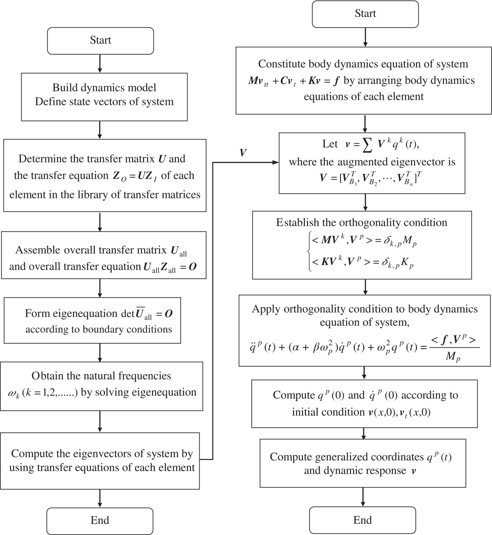
Figure 1.1 Vibration characteristics and dynamics response procedure.
The solution procedure for the MSDTTMM is shown in Figure 1.2 for the dynamics of a general MS that is time‐variant, nonlinear and has large motion and control. First, letting ![]() and taking boundary conditions into the overall transfer equation of the system, the state vectors of the boundary at time ti can be obtained by solving the overall transfer matrix of the system. Then the state vectors of every hinge point and the system dynamics at time ti can be obtained by applying the transfer equations of the elements. Lastly, the time history of the system dynamics can be obtained by letting
and taking boundary conditions into the overall transfer equation of the system, the state vectors of the boundary at time ti can be obtained by solving the overall transfer matrix of the system. Then the state vectors of every hinge point and the system dynamics at time ti can be obtained by applying the transfer equations of the elements. Lastly, the time history of the system dynamics can be obtained by letting ![]() and repeating the above process until the required time T.
and repeating the above process until the required time T.

Figure 1.2 The MSDTTMM procedure.
The order of the system matrix of the MSTMM is much lower than that of the ordinary dynamics method. For example, the order of the system matrix of the chain system is only dependent on the highest order of the matrix of elements. This is the important feature of the MSTMM that differs from the ordinary MSDM. Why does an originally complex matter become so simple? Because the “hinge” and the “body” are considered to have equivalent positions in the MSTMM and therefore it is not necessary to deal with the “hinge” in the way of an ordinary MSDM.
It is necessary to point out that the linear MSTMM is essentially different from the MSDTTMM, which will be discussed in detail in the following chapters.
1.4.3 Features of the Transfer Matrix Method for Multibody Systems
The characteristics of the ordinary MSDM are as follows:
- The global dynamics equations of the system are necessary and are usually hybrid equations composed of ordinary differential equations expressing rigid body motion and partial differential equations expressing flexible body motion, as well as algebraic (or ordinary differential) equations describing constraints. They have to be re‐deduced, which is complex, if the elements of the system change.
- The order of the system matrix is high and usually equal to the number of degrees of freedom of the system, so the computational scale is huge for complex MSD.
- It is complicated to solve the dynamic response of the MRFS because generally most scholars and engineers convert the partial differential equations into ordinary differential equations by using separating variables using the assumed modes method and also convert algebraic equations into ordinary differential equations, then solve them all together; The true mode is unknown in these methods, resulting in a unclear difference between the assumed mode and the true mode, and obviously this affects the solution precision of the dynamic response.
The characteristics of the MSTMM are as follows:
- There is no need for global dynamic equations of the system, so the complex procedures for developing the global dynamics equations will be avoided forever.
- The order of the system matrix is independent of the number of degrees of freedom of the system, for example the order of the system matrix only depends on the highest order of the element matrices for the chain system. The MSTMM has much smaller computational scale and much faster computational speed because of its lower order of system matrix, so the computational ill‐condition of the eigenvalue is avoided.
- Wide application fields and powerful functions. The research objectives of the classical TMM are two kinds of linear elastic structural systems: linear discrete systems composed of springs and lumped masses, and continuous systems composed of elastic solid components. It is hard to deal with general MSs for the classical TMM. The computation of the vibration characteristics of the complex MRFS is easy for the MSTMM and is difficult for ordinary dynamics methods.
- If using the MSDTTMM, MSD can usually be obtained by solving algebraic equations instead of differential equations. The dynamics of linear time‐invariant MSs can be obtained by solving the body dynamics equations of the system. The dynamics of time‐variant MSs can be obtained by solving the transfer equations of the system. It is easy to understand and apply the MSTMM.
- High programming. The overall transfer matrix can be deduced automatically using the transfer matrices of the elements with the standard form according to the topology of the system. Once the transfer matrix has been derived for the given motion and connection model, it can then be used for any MS with the corresponding motion and connection model. In fact, various transfer matrices of elements can be found directly from the transfer matrix library given in this book. The dynamics modeling and analysis of MSs become flexible, concise and quite simple. This work can be done efficiently by a computer because the computational scale is small.
- It is only necessary to solve ordinary differential equations to obtain the dynamic response of an MRFS. The true mode of the system can be obtained with a much higher accuracy either by the TMM for the MRFS or directly by modal test. Thus, a high‐precision dynamic response can be achieved.
Because of these characteristics, the MSTMM has played a very important role in the dynamics design and testing in aeronautics, astronautics, vehicles, robots, machinery etc.
1.5 Launch Dynamics
Launch dynamics [1, 2, 132] is a subject that studies the forces acting on a launch system and the consequent motion of the system during the launching process. It is involved in interior ballistics, external ballistics, middle ballistics, aerodynamics, launch systems dynamics, MSD, vibration theory, test technology, etc. and is closely related to modern science and technology. The theory and technology of launch dynamics have become a research hot topic and increasing attention has been given to the field of modern launch science and technology at home and abroad. This has been one of the main special subjects in all International Symposium of Ballistics and American Guns Dynamics Conferences.
The entire trajectory of a projectile may be divided into two stages: the launching process and free flight. The trajectory of projectile flight with zero attack angles under standard conditions is a plane curve called the ideal trajectory in exterior ballistics [133]. The factors that are not considered in the ballistics equations of an ideal trajectory are called disturbance factors. These factors make the real trajectory deviate from its ideal trajectory. The initial disturbance of a projectile is given by the initial values of the 12 motion parameters of the exterior ballistics equations of a rigid projectile with six degrees of freedom, including three initial rotation angles of initial swing angle Φ0, the initial deflection angle Ψ0, the initial spin angle γ0 and the corresponding angular velocity ![]() ,
, ![]() ,
, ![]() , the initial position coordinate r0 and the corresponding velocity v0 in three directions at the launch end [1]. The initial disturbance of a projectile is caused by the combined effect of various factors in the launch process, for example the projectile, launcher, propellant and environment. The results of study of the initial disturbance of a projectile provide technology support for the design and evaluation of the dynamic performances of a launch system by optimizing the structure parameters. The vibration characteristics of the launch system are one of the main study components of launch dynamics. It has beens proved in practice that a reasonable dynamics model of a launch system should be the MRFS and the tubes of the launch system have to be treated as elastic bodies. For example, the dynamic performance of the MLRS is affected greatly by the ratio of eigenfrequencies to running launch frequencies. In the launch test of a launch system, in order to evaluate the performances scientifically, to decrease the ammunition consumption significantly and to improve the performances of the launch system via the implementation of dynamics design, it is first necessary to compute rapidly the vibration characteristics and exactly analyze the dynamic responses of the MRFS for the launch system. A number of difficulties have to be solved to achieve this. First, too high an order of matrix causes the computation to fail because of the huge computational scale of the vibration characteristics of the MRFS and the inevitable computational ill‐condition problem of a high stiffness gradient system when using ordinary methods. Second, coupling of rigid and flexible bodies causes the non‐self‐conjugate problem of the eigenvalue of the MS and the lack of the orthogonality of the eigenvectors of the system under ordinary means so the modal method cannot be used to analyze exactly the dynamic response of the system.
, the initial position coordinate r0 and the corresponding velocity v0 in three directions at the launch end [1]. The initial disturbance of a projectile is caused by the combined effect of various factors in the launch process, for example the projectile, launcher, propellant and environment. The results of study of the initial disturbance of a projectile provide technology support for the design and evaluation of the dynamic performances of a launch system by optimizing the structure parameters. The vibration characteristics of the launch system are one of the main study components of launch dynamics. It has beens proved in practice that a reasonable dynamics model of a launch system should be the MRFS and the tubes of the launch system have to be treated as elastic bodies. For example, the dynamic performance of the MLRS is affected greatly by the ratio of eigenfrequencies to running launch frequencies. In the launch test of a launch system, in order to evaluate the performances scientifically, to decrease the ammunition consumption significantly and to improve the performances of the launch system via the implementation of dynamics design, it is first necessary to compute rapidly the vibration characteristics and exactly analyze the dynamic responses of the MRFS for the launch system. A number of difficulties have to be solved to achieve this. First, too high an order of matrix causes the computation to fail because of the huge computational scale of the vibration characteristics of the MRFS and the inevitable computational ill‐condition problem of a high stiffness gradient system when using ordinary methods. Second, coupling of rigid and flexible bodies causes the non‐self‐conjugate problem of the eigenvalue of the MS and the lack of the orthogonality of the eigenvectors of the system under ordinary means so the modal method cannot be used to analyze exactly the dynamic response of the system.
It has been proved by theory and experiment that the launch orders of the MLRS have a great influence on its launch dispersion. The reason for this is that different launch orders will result in different vibration characteristics, different initial disturbances and different launch dispersions of projectiles. The vibration characteristics and the ratio of eigenfrequencies to launch frequencies of a running‐fire MLRS have a great influence on its dynamic performance. Rapid and exact computation of the vibration characteristics of the MLRS is of great importance and has become one of the key topics of the launch dynamics of the MLRS. The total mass of rockets is usually larger than the mass of tubes in the MLRS. The mass influences the vibration characteristics of the MLRS, which are different for each rocket. To scientifically evaluate and improve the dynamic performance of the MLRS, it is necessary to find the quantitative relationship between the structural parameters and the vibration characteristics, and match the eigenfrequency with the launch frequencies by changing the structure parameters of the MLRS.
The main methods of studying the vibration characteristics of a system are the FEM, the modal analysis method and the modal synthesis method. The FEM and the MSDM, for example the Wittenburg method and the Kane method, are important in studying launch dynamics. Generally speaking, these methods are efficient for computing complex engineering systems. At the same time, it is usually difficult to study the vibration characteristics of the mechanism system because of the large computational scale of these methods.
It is an urgent requirement in the area of launch dynamics to seek methods to improve the dynamics modeling precision and reduce the computational scale for the dynamics of MSs. Based on the MSTMM, the authors have developed new theory for the launch dynamics of MSs. Many difficult problems related to high‐technique engineering have been solved successfully because the theory of the launch dynamics of MSs developed based on the MSTMM expounds launch dynamics in a totally new way and injects new energy into its development.
1.6 Features of this Book
The characteristics of this book are as follows:
- The MSTMM and its theory system are originated and systemically introduced. A totally new method is obtained to compute MSD with high computational speed and without global dynamics equations of the system.
- The MSTMM is established for linear systems, multi‐dimensional systems, controlled systems, time‐variant MRSs, time‐variant MRFSs, and time‐variant controlled systems. These methods are used for dynamics analysis of linear time‐invariant systems and general time‐variant nonlinear MSs undergoing large motion and control, and provide a powerful means for forecasting the dynamics performances of general mechanical systems.
- Using the new theory and method for the eigenvalue problem and dynamics design provided by the MSTMM, the problems of computational ill‐condition and the huge computational scale of MRFSs arising in important projects have been overcome and computational efficiency has been increased.
- New concepts of augmented eigenvector, augmented operator and body dynamics equations of MSs are presented, and the orthogonality of the eigenvectors of the MRFS proved for the first time. We solve the difficulty of analyzing exactly the dynamic response of the system using the modal method because of the nonself‐conjugation of the eigenvalues of MSs and the lack of orthogonality of the eigenvectors of the system under ordinary means caused by coupling of rigid and flexible bodies. The dynamic response of the MRFS is analyzed precisely and the dynamics design of important engineering products, such as the launch system, etc., is realized.
- The library of transfer matrices of MSs is established for the first time. The transfer matrices of various elements involved in linear system dynamics and general MSs are given systemically. The MS required can be readily assembled by using the transfer matrices of elements in the library and MSD can be studied easily.
- Based on the MSTMM, the theory, technology and simulation systems of the launch dynamics of MSs are established, including the launch dynamics of MLRSs, self‐propelled launch systems and shipboard launch systems, indicating that launch dynamics have entered the practical stage. The initial disturbance theory of a projectile is presented to improve launch precision and decrease experimental consumption of projectiles for launch systems by studying the launch dynamics. This theory is the basis for accurate forecasting and evaluation of the dynamic performance of the launch system.
- Using the MSTMM, technologies for improving the launch precision of the launch system and decreasing projectile consumption in strict tests are presented for the first time.
- The MSTMM and its application results have been appraised by the government appraisal commission that the MSTMM possesses original innovativeness and many proprietary intellectual properties, leads launch dynamics research into practical stage, achieves international leading level, has brought great social, economic and military benefits and has broad application prospects. Professor Rui has given over 50 invited lectures in 16 universities and institutes, and has been invited to international conferences by scientists such as Professor Werner Schiehlen, former President of International Union of Theoretical and Applied Mechanics.
1.7 Sign Conventions
According to the features of the MSTMM, the sign conventions in this book are as follows:
- Mechanics elements. Mechanics elements are classified into two types, “bodies” and “hinges”, and are numbered uniformly. “Bodies” include rigid bodies, flexible bodies, lumped masses, etc. “Hinges” are the links between bodies, including elastic hinges, smooth hinges, prismatic hinges, fixed hinges and damping hinges. A hinge is considered as massless and its mass is totally included in its inboard body and outboard body.
- State vector. For a nonboundary end, the first and second subscripts i and j (
 ) in a state vector zi,j of the end denote the sequence numbers of the adjacent body element and hinge element, respectively. Only one of the boundary ends of a MS is called the root, and all of the other boundary ends are considered as the tips. In the state vectors of boundary ends of root and tips zi,0, the second subscript
  and the first subscript i stand for the sequence number of the elements of root and tips involved.
 - Transfer direction. The transfer direction of a system is always from its tip to its root.
- Input end and output end. Every body element has only a single output end, and all of the other ends are considered as input ends. Along the transfer direction, the nodes entering into the element are called the input ends of the element and are denoted by Ii
 , and the node leaving from the element is called the output end of the element and is denoted by O. There are sometimes several elements in a transfer path. The connection point between elements is the output end of its inboard element and the input end of its outboard element. It is denoted by Pi,j, where the first subscript i indicates the sequence number of the body element and the second subscript j indicates the sequence number of the hinge. Sometimes the connection point Pi,j is denoted by (i, j).
 - Coordinate systems. The stationary inertial Cartesian coordinate system is used to describe the motion of the elements of a multibody system. In order to easily describe the motion of the system, some inertial coordinate systems with different orientations are used according to research objects, and the orientation relations between different coordinate systems are described with direction cosine matrices. The parameters of transfer matrices are described in body‐fixed coordinate systems for a linear time‐invariant system. The origin of the coordinate system of an element is at the input end for an element with a single input end or at the first input end for an element with more than one input end. For a nonlinear, time‐variant system in the MSDTTMM the body‐fixed coordinate system o2x2y2z2 of an element is uniquely determined in the inertial Cartesian coordinate system oxyz. The space‐three axes inertial coordinate system is used as the reference system, and the space‐three angles (1‐2‐3) [71] are used to describe the orientation of the rigid body.
- Position coordinates and coordinates cross‐product matrix. For a rigid body element, C, D and E denote the mass center, the action point of the external force and the torque center of the external torque (torque center for short), respectively. The coordinates of any point of the rigid body in its body‐fixed coordinate system located at its input end are denoted with a column matrix and boldface italic letter l. For example, in the body‐fixed coordinate system of a rigid body, the position coordinates of the output end O are
 , the position coordinates of the mass center C are
  , the position coordinates of the action point D of the external force are
  , and the position coordinates of the torque center E are
  . The coordinates of the input ends
  and the output end O are denoted as
  and
and  , respectively, and these are decomposed in the body‐fixed coordinate system located at the first input end of the body element.
The cross‐product matrix of the position vectors is denoted by the symbol
 , for example(1.1)
- Physical coordinates and modal coordinates of displacement, position coordinate, angular displacement, rotation angle, torque and force. For linear systems, boldface italic lowercase
 ,
,  ,
,  and
and  denote the column matrices of linear displacements, angular displacements, internal torques (except damping torque) and internal forces (except damping force), respectively, of a connection point relative to the equilibrium position of the system in the inertial coordinate system under physical coordinates. Boldface italic capitals
  ,
, 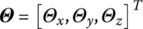 ,
,  and
and 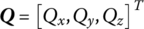 denote the corresponding column matrices of linear displacements r, angular displacements θ, internal torques m and internal forces q, respectively, under modal coordinates.
The physical coordinates can be expressed with modal coordinates as follows:
(1.2)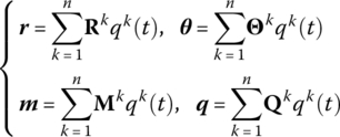
where k denotes the order of the modal, n denotes the number of degrees of freedom of the system, t is time and qk(t) denotes the generalized coordinates.
For general time‐variant and nonlinear MSs,
 ,
,  ,
,  ,
,  ,
,  ,
,  and
and  denote the column matrices of the position vectors of output end O relative to I, rotation angles, internal forces and internal torques of point I relative to the three‐space axes inertial coordinate system and the body‐fixed coordinate system under physical coordinates, respectively.
  and
and 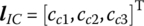 denote the column matrices of the position vectors of mass center C with respect to I in an inertial coordinate system and a body‐fixed coordinate system, respectively, and A denotes the transformation matrix from a body‐fixed coordinate system to an inertial coordinate system. From the definition of a transformation matrix, it can be inferred that
  ,
,  and
and  .
. - Conventions for the positive direction for displacement, position coordinate, angular displacement, rotation angle, torque and force (Figures 1.3 and 1.4). Positive displacements and position coordinates x, y, z and angular displacements and rotation angles θx, θy, θz at the input and output ends coincide with the positive directions of the coordinate system. Inboard forces qx, qy, qz and outboard torques mx, my, mz acting on the elements are positive (negative) if their vectors are in the positive (negative) directions of the coordinate system, and outboard forces qx, qy, qz and inboard torques mx, my, mz acting on the elements are positive (negative) if their vectors are in the negative (positive) directions.
- Bold italic lowercase zi,j and bold italic capital Zi,j denote the state vectors of the connection point Pi,j under physical coordinates and modal coordinates, respectively, that is:(1.3)
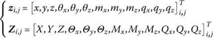
For describing and writing conveniently, bold italic capital ZI and ZO denote the state vectors of the input and output ends, respectively, of the body element with only two ends.
 and
and  denote the state vectors of
  connection points Pi,j,
  ,…,
,…, and Pi,j,
  ,…,
,…,  , respectively, of the body element with more than two ends. Generally speaking, as the state variants of the state vector, displacements include linear displacements and angular displacements, position coordinates include position coordinates and rotation angles, and forces include forces and the torques. To keep things simple, these will not be explained again.
 - Bold italic capital Ui denotes the transfer matrix of the element whose sequence number is i. Bold italic capital Uk,j denotes a partitioned matrix of a transfer matrix, where the subscripts k and j are the sequence numbers of the row and column, respectively, of the partitioned matrix in the transfer matrix. The transfer matrix
 and the partitioned matrix
  are the resultants of continued multiplication of the transfer matrices of all elements in the transfer path from element i to element k of the system. Lowercase uk,j or uk,j denote an element of a transfer matrix, where k and j represent the row and column numbers, respectively, of the element in the transfer matrix.
 - Bold italic capital In denotes a unit matrix of order n, bold italic capital
 denotes a zero matrix with m rows and n columns, and 0n denotes a zero column matrix with n rows.
 - Bold italic capital V denotes an augmented eigenvector of the system, Vk denotes the augmented eigenvector corresponding to the kth order modal and bold italic lowercase v denotes the column matrix of corresponding physical coordinates, that is(1.4)

where
 denotes the kth generalized coordinate, and vt and vtt denote the first‐ and second‐order derivatives of v with respect to time t, respectively, Fi or Fi denotes the external force acting on the ith element, fi denotes the external force (including the external torque) acting on the ith element and f denotes the column matrix of the external force of the system.
 - According to the writing standard that the operators should be expressed using standardized form, the bold capital standardized forms M, K and C denote the augmented operator matrices presented in this book.
- δk,p denotes the Kronecker operator(1.5)
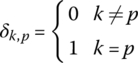
where k and p are natural numbers.
- Bold italic type is used for vectors and matrices.
- The International System of Units (SI) is used in the examples and problems throughout the book. In this system, the three basic units are the meter (distance), the kilogram (mass) and the second (time). The unit of force called the newton is derived from these three basic units.
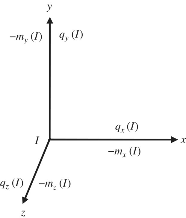
Figure 1.3 Positive direction convention of torques and forces at the input end.

Figure 1.4 Positive direction convention of torques and forces at the output end.