
4
Transfer Matrix Method for Nonlinear and Multidimensional Multibody Systems
4.1 Introduction
Nowadays, nonlinear science is developing rapidly, bringing an unprecedented challenge to almost all disciplines and fields. Any physical system is nonlinear as long as it is analyzed precisely enough. Considering a real physical system as a linear system means that its main performance can be represented precisely enough by an approximate linear system. “Precisely enough” means the difference between the real system and an ideal linear system is so insignificant that it can be neglected for a particular matter. Whether to model a real physical system as linear or nonlinear depends on the specified requirements and conditions.
Essentially, the transfer matrix method for multibody systems (MSTMM) transforms the problems of developing the differential dynamics equation and its solution into problems of developing the transfer equation describing the relation between the state vectors of input and output ends and its solution. The transfer direction is unidirectional and one‐dimensional for the classical transfer matrix method (TMM). The methods for dealing with the tree system, closed‐loop system and framework system, which are common in engineering, are studied in Chapter 11. These are also one‐dimensional methods.
In this chapter, the strategies to solve the dynamics of nonlinear multibody systems by using the MSTMM are introduced. The following topics are included: solving the steady‐state response of a nonlinear system by using the increment MSTMM and iterative algorithms [236] and studying the dynamics response and eigenvalue problem of a nonlinear system by using the finite element transfer matrix method for a multibody system (FE‐MSTMM). The FE‐MSTMM combines the advantages of the FEM (its powerful ability to deal with complex structures) and the TMM (its high computational efficiency). Then the MSTMM for the dynamics analysis of a two‐dimensional system [74, 75] is introduced, which was developed by the authors. A two‐dimensional system is divided into some regions and a transfer direction is chosen, then the state vectors and their transfer relations between the start point and end point in the region are established. The FE‐MSTMM has a higher computational efficiency compared with the FEM and can be extended to three‐dimensional problems.
4.2 Incremental Transfer Matrix Method for Nonlinear Systems
The linearization of a vibration system not only makes the mathematics solution simple, but also provides satisfactory results for many engineering problems. For example, problems such as the physical explanation of resonance phenomena and the relations between the eigenfrequencies or eigenvectors and system parameters etc. can be solved satisfactorily by linear vibration theory. However, such a linearization strategy is sometimes extensively adopted where nonlinear terms are abandoned without verification, resulting in significant computational errors and even essential mistakes. It has been proved by experience that it is impossible to replace the analysis of every vibration system using the linear theory. Even a quasi‐linear system has essential differences compared with a linear one, regarding the theoretical analysis methods and the vibration characteristics.
The incremental TMM [236] for the steady‐state response of nonlinear systems under periodic excitation is introduced in this section. This method is similar to the ordinary TMM, the only difference being that increases in state variables are used to describe the problem and the state variables of the system are extended to Fourier series. The transfer matrix is composed of the increments which are related to Fourier coefficients.
Consider the nonlinear system with n degrees of freedom, as shown in Figure 4.1, which is composed of n lumped masses connected by springs and dampers. The spring and the damper at the left are fixed to the wall (sequence number 0), while the right (sequence number ![]() ) lumped mass 2n is free. Nonlinearity may exist in both the spring and damping characteristics. For convenience, however, we will consider here only cases in which nonlinearity exists in spring characteristics. The mi, Fi and Ω denote the mass of the lumped mass i, force and excitation frequency, respectively. ki,
) lumped mass 2n is free. Nonlinearity may exist in both the spring and damping characteristics. For convenience, however, we will consider here only cases in which nonlinearity exists in spring characteristics. The mi, Fi and Ω denote the mass of the lumped mass i, force and excitation frequency, respectively. ki, ![]() and ci denote the linear part and nonlinear characteristics of the spring coefficients and the viscous damping coefficient of element i, which is composed of springs and dampers. The displacement x and the internal force qx are state variables. Figure 4.2a and b show the analysis of forces of the elements composed of springs and dampers and the lumped mass, respectively.
and ci denote the linear part and nonlinear characteristics of the spring coefficients and the viscous damping coefficient of element i, which is composed of springs and dampers. The displacement x and the internal force qx are state variables. Figure 4.2a and b show the analysis of forces of the elements composed of springs and dampers and the lumped mass, respectively.
Figure 4.1 An n degrees of freedom vibration system.
Figure 4.2 The force analysis of a single component: (a) spring and damper; (b) mass.
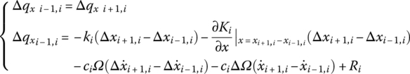
According to the analysis of forces shown in Figure 4.2a, we obtain
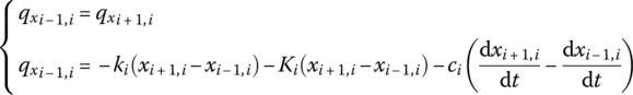
The force analysis in Figure 4.2b yields

Let ![]() , then Equations (4.1) and (4.2) become
, then Equations (4.1) and (4.2) become


where the ‘·’ over x means differentiation with respect to τ.
To develop the incremental method using the TMM for solving Equations (4.3) and (4.4), assume that the stable state response of Ω has the approximate solution (x, qx, Ω). The solution of the linear system or the solution of Ω that is far from the resonant point can be considered as an approximate solution.
We will propose a method which enables us to obtain, starting from this solution, a solution more accurate for a case in which the parameters are kept constant, or a solution valid for a case in which some parameters (here Ω will be considered as a variable parameter) are slightly varied. For instance, we can determine the response curve first by improving the accuracy of an initial solution, and then by obtaining solutions successively for varied Ω. Designate the initial solution as (x, qx, Ω) and try to obtain an improved solution ![]() from this solution. Assume that the improved solution
from this solution. Assume that the improved solution ![]() can be obtained by adding the increment (Δx, Δqx, ΔΩ) to the initial values as follows.
can be obtained by adding the increment (Δx, Δqx, ΔΩ) to the initial values as follows.
Replace (x, qx, Ω) in Equations (4.3) and (4.4) with Equation (4.5), and omit terms with higher order infinitesimals. We obtain

where
are terms retained to improve convergence.
Solving Equations (4.6) and (4.7), (Δx, Δqx, ΔΩ) and the improved solution ![]() can be obtained. Fourier series is used to solve Equations (4.6) and (4.7). The incremental state vector and incremental transfer matrix are introduced according to Equation (4.6).
can be obtained. Fourier series is used to solve Equations (4.6) and (4.7). The incremental state vector and incremental transfer matrix are introduced according to Equation (4.6).
The initial solution in Equation (4.6) is developed into Fourier series of the form:
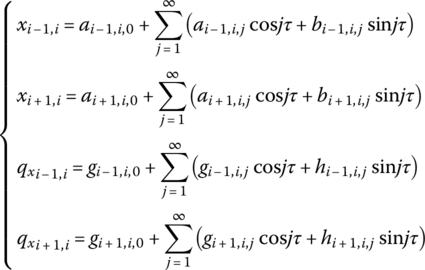
Since the initial solutions ![]() ,
, ![]() ,
, ![]() and
and ![]() are known quantities, the Fourier coefficients a, b, g and h in Equation (4.9) are also known.
are known quantities, the Fourier coefficients a, b, g and h in Equation (4.9) are also known.
Similarly, the unknown increments Δx and Δqx are also extended to Fourier series
where the Fourier coefficients Δa, Δb, Δg and Δh are unknown quantities.
As long as these unknown quantities can be obtained, the increments ![]() ,
, ![]() ,
, ![]() and
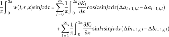
and ![]() can be determined according to Equation (4.10). To determinate these quantities, Equations (4.9) and (4.10) are substituted into Equation (4.6) and applying the harmonic balance principle, we obtain
can be determined according to Equation (4.10). To determinate these quantities, Equations (4.9) and (4.10) are substituted into Equation (4.6) and applying the harmonic balance principle, we obtain

since
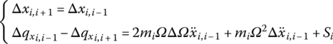
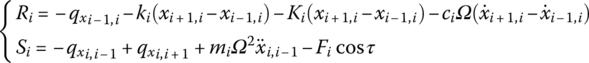
where

Let
then
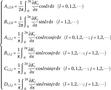
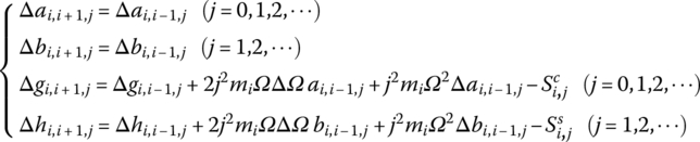
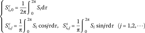
where the Fourier coefficients are given as


therefore
in Equations (4.12a) and (4.12b), ![]() and Ri are obtained by substituting
and Ri are obtained by substituting ![]() into them.
into them.
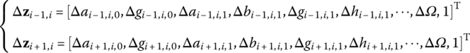
To denote Equation (4.11) in matrix form, define the incremental state vectors at the connection points ![]() and
and ![]() , respectively
, respectively
which are similar to the extended state vectors in the ordinary TMM.
Equation (4.11) is denoted as the incremental transfer equation of a component which is composed of parallel dampers and springs,
where Ui corresponds to the transfer matrix in the ordinary TMM and is called the incremental transfer matrix of the component that is composed of parallel dampers and springs.
Equation (4.11) becomes
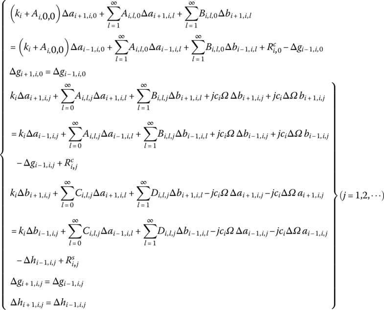
namely
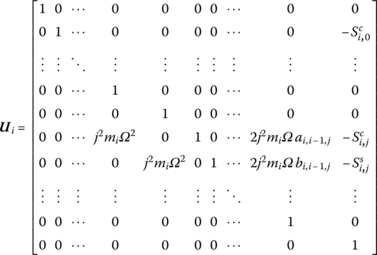
where

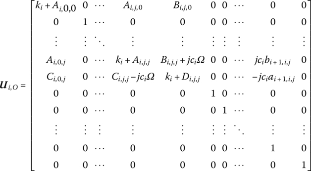
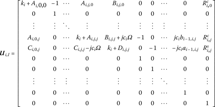
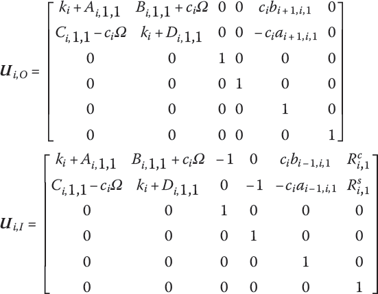
The incremental transfer matrix of the component composed of a parallel damper and spring is
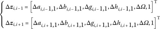
As an example, consider the case in which only the harmonic components are retained. The incremental state vectors in Equation (4.13) are

The corresponding incremental transfer matrix is ![]() , where
, where
According to Equation (4.7) the incremental transfer matrix of the lumped mass is introduced. Similarly, with Equations (4.9) and (4.10) and the harmonic balance principle, Equation (4.7) becomes
where
To express Equation (4.19) in matrix form, incremental state vectors at the connection points ![]() and
and ![]() are defined as
are defined as

Then Equation (4.19) is written as incremental transfer equation of the lumped mass:
where Ui is the incremental transfer matrix of the lumped mass:
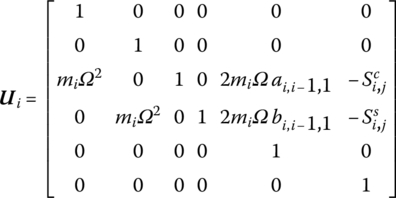
As an example, consider the case in which only harmonic components are retained. The incremental state vectors in Equation (4.21) yield
The corresponding incremental transfer matrix is
Combine Equations (4.14) and (4.22), using the steps of the multibody system TMM to obtain the stable state response of a multi‐degree‐of‐freedom system. Thus, the incremental TMM has been fully established. To explain how to use this method, in the following the solution process of the steady‐state response for n degrees of freedom (DOF) system will be introduced, as shown in Figure 4.1. According to the system structure, the state vectors Δz0,1, Δz2,1, Δz2,3, Δz4,3, Δz4,5, …, ![]() are defined in the same form as Equations (4.13) or (4.21), and the transfer equation yields
are defined in the same form as Equations (4.13) or (4.21), and the transfer equation yields
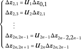
where U1, U3, ![]() are the incremental transfer matrices of components 1, 3, …,
are the incremental transfer matrices of components 1, 3, …, ![]() , respectively, which are composed of parallel dampers and springs. U2, U4 and U2n are the incremental transfer matrices of lumped masses 2, 4, …, 2n, respectively.
, respectively, which are composed of parallel dampers and springs. U2, U4 and U2n are the incremental transfer matrices of lumped masses 2, 4, …, 2n, respectively.
The overall transfer equation is obtained by successively multiplying each transfer matrix in sequence
where U is the overall transfer matrix.
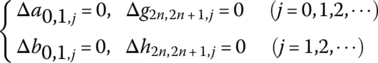
From the boundary conditions, parts of the state variables in Δz0,1 and ![]() are zeros, that is
are zeros, that is
Therefore, the problem is simplified to solve Equation (4.27) under the condition of Equation (4.28). Solving Equation (4.27), the unknown state variables in Δz0,1, ![]() and the boundary incremental state vectors Δz0,1 and
and the boundary incremental state vectors Δz0,1 and ![]() can be determined. Finally, the state vectors of all the connected points can be obtained through the transfer equations of all components. Substituting these increments into the initial solution, according to Equations (4.10) and (4.5), the improved solution can be evaluated. If this improved solution cannot satisfy the accuracy, take the improved solution as the new initial solution, and the new increments can be evaluated by repeating the process to solve Equation (4.27) until the improved solution satisfies the accuracy.
can be determined. Finally, the state vectors of all the connected points can be obtained through the transfer equations of all components. Substituting these increments into the initial solution, according to Equations (4.10) and (4.5), the improved solution can be evaluated. If this improved solution cannot satisfy the accuracy, take the improved solution as the new initial solution, and the new increments can be evaluated by repeating the process to solve Equation (4.27) until the improved solution satisfies the accuracy.
As an example, take Equation (4.18) as the incremental transfer matrices of the component composed of parallel dampers and springs, and Equation (4.25) as the incremental transfer matrices of the lumped mass, respectively. Using the boundary conditions in Equation (4.28), Equation (4.27) becomes
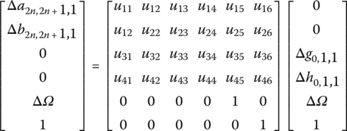
where uij is the element of the overall transfer matrix.
Let ![]() in Equation (4.29). A more precise improved solution corresponding to the original excitation frequency Ω can be found by solving Equation (4.29). If this improved solution still does not satisfy the precision, the repeated step could be carried out. If
in Equation (4.29). A more precise improved solution corresponding to the original excitation frequency Ω can be found by solving Equation (4.29). If this improved solution still does not satisfy the precision, the repeated step could be carried out. If ![]() is a given value in Equation (4.29), the improved solution corresponding to excitation frequency
is a given value in Equation (4.29), the improved solution corresponding to excitation frequency ![]() can be obtained. If this improved solution still does not satisfy the precision, repeat the same step.
can be obtained. If this improved solution still does not satisfy the precision, repeat the same step.
4.3 Finite Element Transfer Matrix Method for Two‐dimensional Systems
FEM is the most widely used and powerful tool for structural analysis. However, many nodes used in a very complex structure induce huge matrices which need to be managed and dealt with. The computation cost is huge, and systems with large stiffness gradients usually are accompanied by computational “ill‐condition”, which leads to computational difficulties. Therefore, the problem of how to increase the computation speed and avoid computational “ill‐condition” is one of the eternal topics for FEM research. The two‐dimensional structure is divided into finite regions along the transfer direction, and each region is divided again into finite elements. FEM is used to develop the matrix relations of state variables at the two ends of strips. Consequently, it is solved by the TMM. The FE‐TMM can be developed [237] by combining the FEM with the TMM, which greatly reduces the computational costs compared with using the FEM only. The FE‐TMM has not only the strong power of the FEM, but also the high efficiency of the TMM in dealing with complicated structures.
4.3.1 Differential Equation of the Transverse Vibration of a Thin Plate
The object enclosed in the surfaces of two parallel planes and a vertical cylinder or prism is called a flat plate, or simple plate, in elastic mechanics where the thickness is much less than the size of the bottom surface, as shown in Figure 4.5. h is the thickness of the plate. The middle plane that bisects the thickness h is a neutral surface. The neutral surface is assumed to coincide with the oxy plane and the z axis is vertical downwards. The displacements of any point along the x, y and z axes are denoted by u, v and w, respectively.
Figure 4.5 Rectangular element of a plate.
Assuming that the original cross‐section is still a plane after deformation, this yields
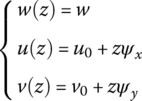
where u0 and v0 are the displacements of elements on the neutral surface of the plate, ψx is the angular displacement around the x axis and ψy is the angular displacement around the y axis.
Shear deformations are
where γxz is the angular displacement of element dxdz and γyz is the angular displacement of element dydz.
Figure 4.5b shows the forces on the element dxdy under transverse vibration. P is the exciting force distributed on the unit area, ρ is the material density and ![]() is the inertial force on the unit area. According to the condition of moment equilibrium along the y and x axes, and the condition of force equilibrium along the z axis on the rectangular element, the equilibrium equations are
is the inertial force on the unit area. According to the condition of moment equilibrium along the y and x axes, and the condition of force equilibrium along the z axis on the rectangular element, the equilibrium equations are
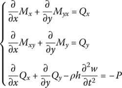
where
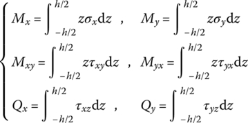
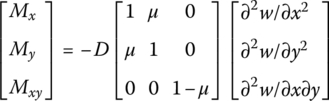
Mx and My are the bending moments, Myx and Mxy are the rotational moments, and Qx and Qy are the shear forces.
If the ratio of thickness to the least character size of the plate is greater than 1/5, the plate is called a thick plate, while if the ratio of thickness to the least character size of the plate is less than 1/80, the plate is called a membrane plate. If the ratio of thickness to the least character size of the plate is between 1/5 and 1/80, the plate is called a thin plate. For a thin plate, bending deformation is mainly generated when all the outside loads are vertical to the neutral surface, and the displacements along the z axis of all the points on the neutral surface are called deflections of the plate. If the ratio of deflection to thickness is less than or equal to 1/5, the problem belongs to small deflection theory.
Kirchhoff’s hypothesis is fundamental assumptions in the development linear elastic, small‐deformation theory for the bending of thin plates. The assumptions are:
- The straight lines, initially normal to the middle plane before bending, remain straight and normal to the middle plane during the deformation, and the length of such an element does not alter. Due to the assumption,
 ,
,  and
and  .
. - σz, the stress normal to the middle plane, is small compared with other stress components (σx, σy and τxy) and may be neglected in the stress–strain relations.
- When the thin plate is bending and deforming, all the points in the neutral surface have only vertical displacement w but no displacement along the x and y axes, that is,
 ,
,  , and
, and  .
.
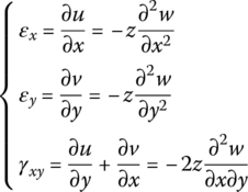
Now deduce the differential equation of the transverse vibration of a thin plate. From Kirchhoff’s hypothesis ![]() and Equation (4.31)
and Equation (4.31)
Equations (4.32) and (4.33) still apply. Considering bending deformation only, Equation (4.30) becomes
then
The stress–strain relation of the thin bending plate is
Substituting Equation (4.37) into Equation (4.33) and taking the integration, we obtain
where 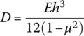 is the bending stiffness of the thin plate.
Substituting Equation (4.38) into the first two formulas of Equation (4.32) yields
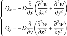
Substituting Equation (4.39) into the last formula of Equation (4.32), the dynamic differential equation of the thin plate is obtained as
where Δ2 is the operator 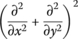 .
.
4.3.2 Triangular Elements
Triangular or rectangular elements are usually used while analyzing the transverse vibration of a thin plate using the FEM. Using three nodal triangular elements and local Cartesian coordinates, the oxy plane is assumed to coincide with the neutral surface of the thin plate. As shown in Figure 4.6, the three nodes are numbered in sequence, and the oy axis is coincident with the line connected by nodes ① and ②.

Figure 4.6 Triangle element of a thin plate.
In each node, displacement w and angular displacements θx and θy are denoted by δ

The displacement vector of the element is
and the nodal force is
where Wi is the force along the z axis, and ![]() and
and ![]() are the nodal moments. These parameters do not have simple relations with the bending moment Mx of this node, and their dimensions are also different.
are the nodal moments. These parameters do not have simple relations with the bending moment Mx of this node, and their dimensions are also different.
The element displacement δe has nine unknown quantities. Therefore, the function of displacement includes nine parameters that have symmetry with respect to x and y. Normally, let
where
a is an unknown constant column vector that is determined by the nodal state of the element, that is

We obtain
where
![]() can be evaluated from Equation (4.48), and substituting this into Equation (4.44) yields
can be evaluated from Equation (4.48), and substituting this into Equation (4.44) yields
where N is a matrix of shape functions
In Equation (4.50), the deflection function w(x, y) of the element is denoted by nodal displacement. In order to deduce the stiffness matrix, Equation (4.50) is substituted into Equation (4.36) and the strain vector of the element expressed by the nodal displacement can be determined as
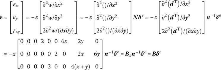
where
The stress vector of the element denoted by nodal displacement can be obtained from Equation (4.37)
4.3.3 The Finite Element Dynamic Equation of a Thin Plate
All the nodal displacements of the whole elements of a thin plate are taken to be generalized coordinates of the thin plate and the Lagrange equation is used to set up the dynamic equation. With Equation (4.50), the deflection function becomes
The kinetic energy of the thin plate is calculated by neglecting the contributions of the in‐plane displacement components u and v, namely

where

Me is the consistent mass matrix of the thin plate element, ρ is the material density and ρh is the mass of the unit area.
The elastic potential energy of an element can be determined from Equations (4.52) and (4.54)
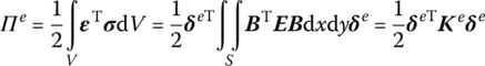
where
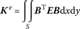
Ke is called the stiffness matrix of the thin plate element.
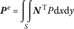
If there is a distributed load P(x, y, t) acting on the element and it is vertical to the plane, according to the principle of virtual work the nodal load is
To develop the overall equation, the expression of each element in local coordinates has to be transformed into global coordinates. Here we only need to transfer Me and Ke by the following transfer matrix
where
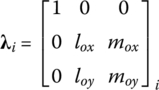
(lox, mox) and (loy, moy) are the direction cosines of local coordinates ox and oy in the global coordinates, respectively.
After the coordinate transformation, the kinetic and potential energies of the whole system, expressed by generalized coordinates of the global nodal displacement, are obtained. The transferred matrices are also denoted by Me and Ke for simplicity, that is
where δ is ![]() ‐dimensional column matrix of displacement of n nodes in turn, and M and K are
‐dimensional column matrix of displacement of n nodes in turn, and M and K are ![]() ‐dimensional matrices.
‐dimensional matrices.
As T and Π are quadratic homogeneous polynomials, M and K can be constructed by adding the related terms together. Because the parameters of one point are only related to its surrounding elements, M and K are sparse diagonally dominant matrices.
Using the Lagrange equation
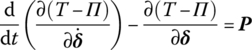
the differential equation of motion of the whole thin plate established by FEM is
As mentioned before, the direction of Pe is the same as the direction of nodal displacement, therefore P is the column matrix of the generalized force of the system.
To obtain the eigenfrequency of a thin plate under the condition of small amplitude, let
Substituting this into Equation (4.66) and assuming ![]() , the free vibration equation becomes
, the free vibration equation becomes
where Φ is the eigenvector.
4.3.4 Finite Element Transfer Matrix Method of Two‐dimensional Systems
Now we take a rectangular thin plate as an example of the analysis steps for the FE‐TMM. As shown in Figure 4.7a, the neutral surface is coincident with the oxy plane, taking the x axis as the transfer direction and dividing the plate into n equal strips along the transfer direction. Dividing each strip into ![]() triangular elements, gives 2m nodes and
triangular elements, gives 2m nodes and ![]() degrees of freedom. According to the TMM, for the ith strip the column matrix of nodal displacement of the AD side is the state vector of the input end, and the BE side is the output end. If the plate is not rectangular, to compute this easily let the index of the state vector of the input and output ends be equal. Of course, other methods exist, such as generalized inverse matrix [238].
degrees of freedom. According to the TMM, for the ith strip the column matrix of nodal displacement of the AD side is the state vector of the input end, and the BE side is the output end. If the plate is not rectangular, to compute this easily let the index of the state vector of the input and output ends be equal. Of course, other methods exist, such as generalized inverse matrix [238].

Figure 4.7 Finite element partition of a thin plate.
Obviously, the input end of the ith strip is the output end of the ![]() th strip. The subscript
th strip. The subscript ![]() is used to denote the input end of the ith strip and the subscript
is used to denote the input end of the ith strip and the subscript ![]() is used to denote the output end of the ith strip. In short, the section between the ith strip and the
is used to denote the output end of the ith strip. In short, the section between the ith strip and the ![]() th strip can be defined as the ith section. The subscript
th strip can be defined as the ith section. The subscript ![]() is used to denote the output end of the ith section and the subscript
is used to denote the output end of the ith section and the subscript ![]() is used to describe the input end of the ith section. The external force acting on the ith strip is ignored and the external force on the ith strip only acts on the nodes in the section.
is used to describe the input end of the ith section. The external force acting on the ith strip is ignored and the external force on the ith strip only acts on the nodes in the section.
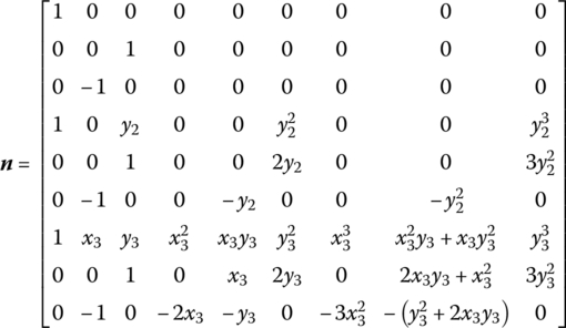
The characteristics of the FE‐TMM include the fact that it is not necessary to develop the dynamic equation of the whole system and only the finite element equation of strips needs to be developed. Taking the ith strip as an example, after dividing it into right‐angled triangle elements, as shown in Figure 4.7b, it is easy to see that the matrix n is nonsingular. According to the boundary conditions of the top and bottom sides of the thin plate, the rows and columns which correspond to the displacement variables can be omitted, with 0 DOF at the plate boundaries (take the simply supported end w as an example) while developing M and K.
Assuming the boundary conditions of top and bottom sides are consistent, the conditions of each strip are the same. The force that acts on the nodes of the input end of element i is taken to be the nodal load of element ![]() , and the force acting on the nodes of the output end of element
, and the force acting on the nodes of the output end of element ![]() is taken to be the nodal load of element i. These two forces are equal and opposite. The column matrices of displacement are denoted by
is taken to be the nodal load of element i. These two forces are equal and opposite. The column matrices of displacement are denoted by ![]() and
and ![]() . The equilibrium equation of the ith strip is
. The equilibrium equation of the ith strip is
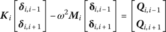
where
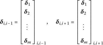
These matrices are ![]() ‐dimensional. If there exist zeros in δ1 and δm, they are omitted.
‐dimensional. If there exist zeros in δ1 and δm, they are omitted.
Simplifying Equation (4.69), this yields
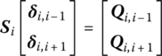
where ![]() is the dynamic matrix of the ith strip.
is the dynamic matrix of the ith strip.
After partitioning we obtain
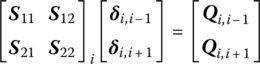
and through simple calculation this gives
where

4.3.5 Solving Vibration Characteristics using the Finite Element Transfer Matrix Method
External load is not considered while computing the free vibration, that is to say, there is no external load at the section (node). Considering the displacement of the two ends of the section is continuous, this yields
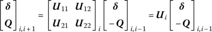
Substituting Equation (4.75) into Equation (4.73), and denoting ![]() , the transfer equation yields
, the transfer equation yields
Finally, the overall transfer equation of the thin plate is
After partitioning U, this becomes
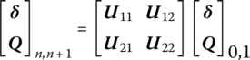
Introducing the boundary condition of two sides, the frequency equation is obtained. For instance, the left side is fixed and right side is free, which means
Substituting into Equation (4.78) yields
so the frequency equation is
When one order frequency is determined, Q0,1 and state vector Z0,1 can be evaluated from Equations (4.80) and (4.79), respectively, and then Z1,2 is obtained from Equation (4.76), so all the state vectors can be determined in turn.
4.3.6 Steady‐state Response using the Finite Element Transfer Matrix Method
When computing the steady‐state response, suppose the external loads only act on the section (node). Considering the displacement of the two ends of the section to be continuous, P denotes the vector of the generalized external force column matrix, and so according to Equation (4.75)

Substituting the equation above into Equation (4.73) leads to
or
Let ![]() , so we have
, so we have
where
4.4 Finite Element Riccati Transfer Matrix Method for Two‐dimensional Nonlinear Systems
The analysis of a geometrically nonlinear structure has been a subject of considerable interest for several decades. When dealing with the transient analysis of structures with large displacement under general excitation by a direct integration method such as the Wilson‐ θ method on a computer, the matrices obtained by the FEM are usually very large, which leads to low computational efficiency. For this reason, various techniques have been suggested to reduce the order of the matrices. The FE‐TMM, introduced in the previous section is one of these techniques. In this method, the size of the stiffness and mass matrices is equal to the number of the degrees of freedom in the subsystem, hence these matrices are much smaller than those obtained by the ordinary FEM. This method has been successfully applied to various linear static, free vibration, dynamic response and nonlinear static problems. By combining the FE‐TMM and the Riccati TMM [225], we can carry out the transient analysis of nonlinear structure dynamics with large displacement under general excitation, where the time integration of the incremental equations could be solved by the Wilson‐θ method. The improved Newton–Raphson method is employed in equilibrium iterative procedures of each time step, and the Riccati transformation of the state vector is proposed to avoid the propagation of round‐off errors occurring in recursive multiplications of the transfer matrices.
4.4.1 Incremental Equilibrium Equation and Direct Integration Method
The governing equation for a dynamic problem in FEM at time t is
where M and C are mass and damping matrices, and ![]() ,
, ![]() , F(t) and R(t) are the acceleration, velocity, nodal elastic force and nodal external force vectors, respectively, of all the nodes of the system at time t.
, F(t) and R(t) are the acceleration, velocity, nodal elastic force and nodal external force vectors, respectively, of all the nodes of the system at time t.
At time ![]() (Δt is the time step, θ is the parameter that for stability control, θ≥1), from Equation (4.87) we can get
(Δt is the time step, θ is the parameter that for stability control, θ≥1), from Equation (4.87) we can get
Equation (4.88) is a nonlinear equation for a geometrically nonlinear structure problem. In the analysis of nonlinear structures, the linearization of equations of motion usually uses the following approximation
where Δv is the vector of incremental displacement in time interval θΔt, with ![]() , and KT(t) is the tangent stiffness matrix at time t [225].
, and KT(t) is the tangent stiffness matrix at time t [225].
Substituting Equation (4.89) into Equation (4.88) and then subtracting Equation (4.87) gives the incremental equilibrium equation from time t to ![]()
where ![]() .
.
Solve Equation (4.90) using the Wilson‐θ method [242]. The Wilson‐θ method is based on the linear acceleration method, namely an assumption is made that the acceleration varies according to the linear rule in time ![]() , as shown in Figure 4.10.
, as shown in Figure 4.10.
Figure 4.10 Assumption of the linear variation of acceleration.
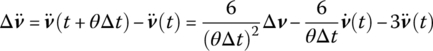
τ is a time variable start from time t, and for 0≤τ≤θΔt the acceleration inside this range can be obtained according to the linear assumption of acceleration
Integrating Equation (4.91) yields
In Equations (4.92) and (4.93), let ![]() , then we obtain
, then we obtain
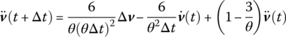
The acceleration and velocity at time ![]() can be determined from Equations (4.94) and (4.95)
can be determined from Equations (4.94) and (4.95)
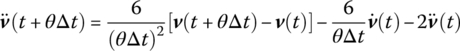
namely
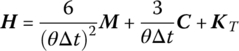
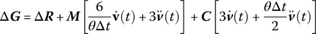
Substituting Equations (4.98) and (4.99) into Equation (4.90) yields
where
Equation (4.100) only has one unknown variable Δv, and we can solve it to obtain the acceleration, velocity and displacements of all the nodes in the system at time ![]()
It is necessary to point out that Δv obtained from Equation (4.100) is only an approximation of incremental displacements. To obtain a more precise solution, a series of iterations is generally used, and the determined solutions Δv, ![]() and
and ![]() are substituted into Equation (4.90), then the approximation of incremental vectors of external force can be obtained:
are substituted into Equation (4.90), then the approximation of incremental vectors of external force can be obtained:
The difference between the real incremental vector of external force and the approximation of external force is called the unbalanced force:
Replacing ΔG in Equation (4.100) by δΔR, we obtain
and the correction δΔv, hence
However, because Δv in Equation (4.100) has a large number of elements, the order of the corresponding matrix H is very large, and this iterative process needs a lot of computation time. Take the thin plate shown in Figure 4.11 as an example. If the plate is divided into n strips, and each strip is divided into 2m triangular elements, then the elements number of Δv is ![]() while the corresponding matrix H is a square matrix with
while the corresponding matrix H is a square matrix with ![]() orders.
orders.
Figure 4.11 Finite element partition of a plane plate.
4.4.2 Finite Element Riccati Transfer Matrix Method for Two‐dimensional Nonlinear Systems
Without loss of generality, consider the plate shown in Figure 4.11.
4.4.2.1 Transfer Matrix of a Strip
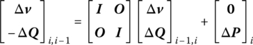
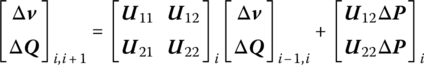
Ignore the external load acting on the ith strip and consider that the external load acts only on nodes, then the transfer equation [226] of the ith strip is
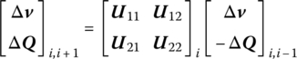
where
![]() ,
, ![]() and
and ![]() ,
, ![]() are incremental vectors of displacement and nodal elastic force on the output ends and input ends of the ith strip from t to
are incremental vectors of displacement and nodal elastic force on the output ends and input ends of the ith strip from t to ![]() , and H11, H12, H21, H22 are the submatrices of matrix H (local) in Equation (4.100).
, and H11, H12, H21, H22 are the submatrices of matrix H (local) in Equation (4.100).
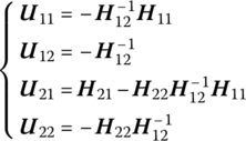
The transfer matrix of the ith section is
where, ![]() ,
, ![]() ,
, ![]() and
and ![]() are incremental vectors of displacement and nodal elastic force on the input ends of the ith strip and the output ends of the
are incremental vectors of displacement and nodal elastic force on the input ends of the ith strip and the output ends of the ![]() th strip from t to
th strip from t to ![]() , and ΔP is the generalized load incremental vector acting on the ith section.
, and ΔP is the generalized load incremental vector acting on the ith section.
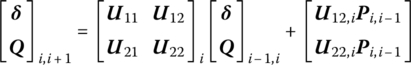
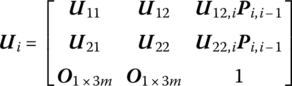
Substituting Equation (4.107) into Equation (4.106) yields
or
Equation (4.108) describes the relation of incremental state vectors of the sections ![]() and i, which is usually described as follows
and i, which is usually described as follows

or
Equation (4.109) is the transfer equation of the ith strip and Ûi is the transfer matrix of the ith strip.
Δv can be obtained from Equation (4.109) by using the ordinary TMM with boundary conditions. Both Equations (4.109) and (4.100) can be applied to achieve Δv: using Equation (4.100) we only need to solve a single large equation once, while using Equation (4.109) we need to solve all the transfer equations step by step to get ![]() . However, the order of corresponding matrix H of Equation (4.109) is much less than the order of the matrix when using Equation (4.100). Taking Figure 4.9 as an example, if Equation (4.109) is used the dimension is only
. However, the order of corresponding matrix H of Equation (4.109) is much less than the order of the matrix when using Equation (4.100). Taking Figure 4.9 as an example, if Equation (4.109) is used the dimension is only ![]() , which is much less than the dimension of H, which is
, which is much less than the dimension of H, which is ![]() .
.
4.4.2.2 Riccati Transformation of Incremental State Vectors
To reduce the propagation of round‐off errors in the ordinary TMM, the Riccati transformation of incremental state vectors is proposed. Rearranging and repartitioning Equation (4.109) we obtain
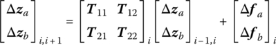
where Δza contains half of the elements, which are already known, of incremental state vectors at the input boundary and Δzb contains the other half of the unknown incremental state variables.
A general Riccati transformation at the ith section is
where Si is the Riccati transfer matrix and vector Δei is associated with external force. From Equations (4.110) and (4.111), we obtain
where
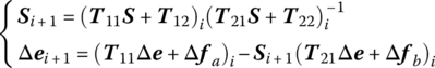
Equation (4.113) shows the general recursive relations for Si and Δei.
First, S1 and Δe1 are obtained by using the input boundary conditions. Then Si and Δei of the whole structure can be obtained in turn by using Equation (4.113), hence
According to the output boundary conditions (parts of state variables are known in ![]() ), by substituting these variables into Equation (4.114) the unknown state variables in
), by substituting these variables into Equation (4.114) the unknown state variables in ![]() can be evaluated. After the incremental state vector
can be evaluated. After the incremental state vector ![]() at the output boundary of the whole structure has been solved, the incremental state vector
at the output boundary of the whole structure has been solved, the incremental state vector ![]() on any section i can be evaluated from Equations (4.114) and (4.111) as follows
on any section i can be evaluated from Equations (4.114) and (4.111) as follows
4.4.2.3 Iterative Procedure
Because the approximation of Equation (4.89) was used, the incremental state vectors obtained from the above are only approximations of the accurate incremental state vectors. Hence, a modified Newton–Raphson method is applied to iterate for dynamic equilibrium equations. The iterative procedure is as follows:
- Let initial Δv(0) be equal to the solution of Equation (4.100) or the solution of TMM in (1),
 .
. - The unbalanced force δΔR(j) is calculated using the following equation
(4.116)

- Replacing ΔG in Equation (4.100) by δΔR(j), we obtain
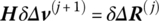
Using FE‐RTM as described above, the
 th correction
  is obtained.
 - The correction
 is added to Δv(j) to obtain the jth approximation
-
 .
. - Repeat iterations (2)–(5) until the unbalanced forces become sufficiently small.
- Using Equations (4.103)–(4.105), the displacement, velocity and acceleration at time
 are obtained.
4.4.3 Numerical Examples
To review the computational accuracy and efficiency of the finite element Riccati TMM, this method is used to compute the dynamic response of armor plate with and without stiffeners under impact load, and these results are compared with those obtained by ordinary FEM.
4.5 Fourier Series Transfer Matrix Method for Two‐dimensional Systems
The Fourier series TMM combines the Fourier series and the TMM, and extends the bivariate function f(x, y) to the following form using a double Fourier series:
fm(y) and gn(x) are usually selected to be trigonometric function systems when they are adopted to solve a two‐dimensional problem of elastic bodies. If the y axis is chosen as the transfer direction, fm(y) is only required to ensure continuous differentiable conditions and gn(x) still belongs to the trigonometric function system. Because of the orthogonality of the function gn(x), a partial differential equation can be transformed into an ordinary differential equation about the y axis, and then the transfer matrix about function fm(y) can be determined.
The temperature change inside an elastic body can bring expansion or shrinkage of its volume. The stress inside an elastic body due to the change of temperature is called thermal stress. In the following, the problem of the thermal stress of a thin plate is used to illustrate the Fourier series TMM.
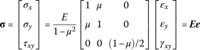
The problem of the thermal stress of a thin plate is a plane stress problem. The displacements and stresses of elements in thin plates are shown in Figure 4.16. Here, u is the displacement along the x axis, v is the displacement along the y axis, ![]() ,
, ![]() are angular displacements, σx, σy are normal stresses of the x and y axes, and τxy, τyx are the corresponding tangent stresses. According to the assumption of plane stress in elastic mechanics, when the external force is zero, the equilibrium equations of the elements are
are angular displacements, σx, σy are normal stresses of the x and y axes, and τxy, τyx are the corresponding tangent stresses. According to the assumption of plane stress in elastic mechanics, when the external force is zero, the equilibrium equations of the elements are
Figure 4.16 Displacement and stress of the element of a thin plate.
Normal strains εx, εy and shear strains γxy are
Assume the height of plate is h. If the linear elastic material is isotropic, the relationships between thermal stress and stain are
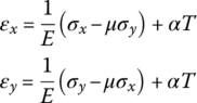
where E is Young’s modulus, μ is Poisson’s ratio, T is the variable of temperature (![]() ) and α is the linear thermal expansion coefficient of an elastic body.
) and α is the linear thermal expansion coefficient of an elastic body.
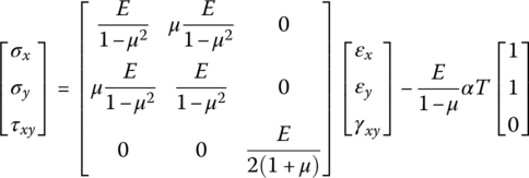
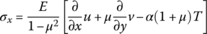
The expressions of the stress components in terms of strain components can be obtained by solving Equation (4.119):
The stress of the difference in temperature of a rectangular thin plate is considered. Its two sides are free along the x axis and its displacement along the y axis can be ignored, as shown in Figure 4.17. If the y axis is the transfer direction, the terms on the left‐hand side of equation are derivatives with respect to y. The derivatives with respect to x are on the right‐hand side of the equation. At first, the following equation can be obtained from Equation (4.118) and the third equation of Equation (4.120)
Figure 4.17 Temperature difference in the stress of a thin rectangle plate.
From the second formula of Equation (4.120),
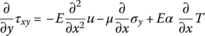
From the second formula of equilibrium Equation (4.117),
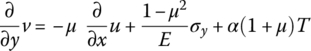
Hence, the three equations about u, v, σy and τxy have been found. To find ![]() , the following equation can be obtained from the first formula of Equation (4.120)
, the following equation can be obtained from the first formula of Equation (4.120)
Substituting Equation (4.122) into the above equation
Substituting Equation (4.124) into the first formula of Equation (4.117) and using the third equation of Equation (4.117)
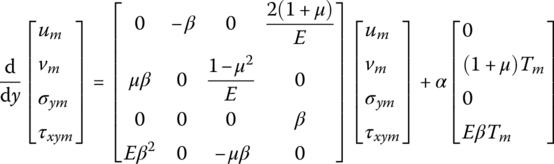
Combining Equations (4.121) to (4.123) and Equation (4.125), we can obtain the partial differential equations
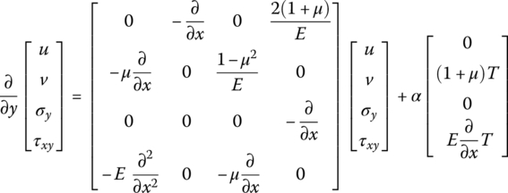
These equations do not now contain σx and the explicit Equation (4.124) of σx has been obtained. After solving the other variables, σx can be determined directly by substituting into Equation (4.124). All the nonzero elements of the matrix can be arranged in the black squares of a chessboard (see section 10.8). This arrangement can bring computational advantages.
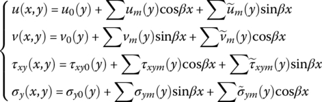
The unknown functions in Equation (4.126) of a rectangular thin plate can be extended to Fourier series
and
where ![]() , L is the width of the thin plate in the x axis and m is the ordinal number of the series term.
, L is the width of the thin plate in the x axis and m is the ordinal number of the series term.
The varying temperature field can be denoted as
The external load at boundary ![]() can be described as
can be described as
More simply, assume the temperature field T(x, y) and external load P(x) are symmetric about center line ![]() of the thin plate, so
of the thin plate, so ![]() and
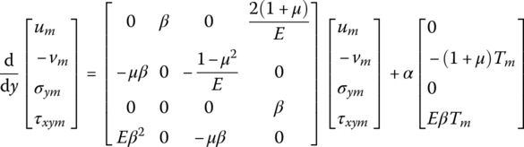
and ![]() , u(x, y) and τ(x, y) are anti‐symmetric about the center line, and the rest are symmetric. According to the boundary conditions, all the terms marked with wave lines are equal to zero; we can obtain the ordinary differential equations about the series coefficients using the orthogonality of the trigonometric series
, u(x, y) and τ(x, y) are anti‐symmetric about the center line, and the rest are symmetric. According to the boundary conditions, all the terms marked with wave lines are equal to zero; we can obtain the ordinary differential equations about the series coefficients using the orthogonality of the trigonometric series
and the mth term of series of normal stress σx
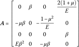
Replacing vm with ![]() , and letting the matrix of the system be symmetric about the minor diagonal
, and letting the matrix of the system be symmetric about the minor diagonal
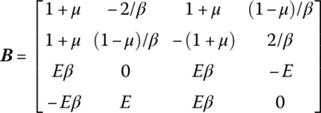
Let
Its Jordan standard form is
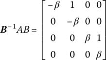
where B is the transformation matrix
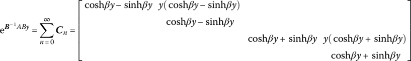
Therefore, the general term of ![]() is
is

After summing, this yields
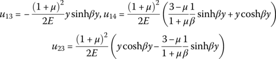
Therefore the transfer matrix of the coefficients in a Fourier expansion of internal displacement and stress of the thin plate with load acting on the edge is
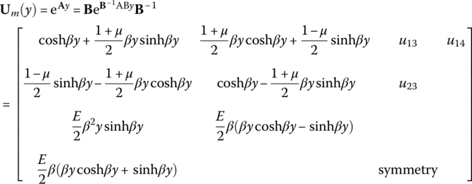
where
Define the state vector as
To obtain the corresponding coefficients of the extended function of stress due to temperature difference, the nonhomogeneous solution of Equation (4.133) needs to be found
where Fm(ξ) is the nonhomogeneous column matrix in Equation 4.133.
If temperature difference is linearly distributed
The nonhomogeneous terms are

Note that ![]() (namely
(namely ![]() ), which can be obtained merely by adding a minus sign to each element in the black grids in matrix
), which can be obtained merely by adding a minus sign to each element in the black grids in matrix ![]() .
.
The coefficient of the series term of normal stress is
4.6 Finite Difference Transfer Matrix Method for Two‐dimensional Systems
The finite difference TMM is a method which combines the finite difference method and he TMM. Again taking the problem of the thermal stress of the rectangular thin plate as an example, consider the y axis as the transfer direction and replace derivation with the finite difference method in the x axis. Herein the plane is not divided into grids, but into strips along the transfer direction, so this method is also called the strip method.
As shown in Figure 4.18, the plate is divided into n areas by ![]() parallels with equal width in a thin plate structure whose boundaries are
parallels with equal width in a thin plate structure whose boundaries are ![]() and
and ![]() . The distance between parallels is Δx. According to the variables found in differential Equation (4.126) in section 4.5, the variables in each parallel are defined as follows:
. The distance between parallels is Δx. According to the variables found in differential Equation (4.126) in section 4.5, the variables in each parallel are defined as follows:
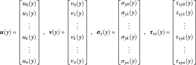
Figure 4.18 Strip element partition of a thin plane rectangle plate.
The derivative of x is denoted in the form of an intermediate difference
At the boundaries ![]() and
and ![]() , the forward and backward differences are applied, respectively, that is
, the forward and backward differences are applied, respectively, that is
To ensure difference accuracy, the extension of the forward and backward difference of the second‐order derivative is
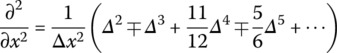
where Δ is the difference operator. Two formulas are involved in the above equation, where the first formula corresponds to the forward difference operator while the second formula corresponds to the backward difference operator.
If only the first two terms are chosen, this becomes
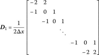
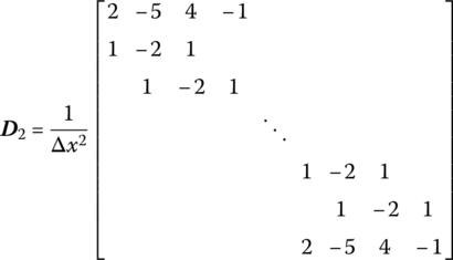
The partial derivatives of v(y), τxy(y) and τxy(y) with respect to x are calculated in the same way as used in the above equations. Therefore, the first‐order difference matrix D1 can be written from Equations (4.146), (4.148) and (4.149), and the second‐order difference matrix D2 can be written from Equations (4.147), (4.151) and (4.152):
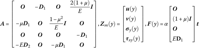
Replacing derivation with finite difference, and considering Equation (4.126), we can obtain the differential equations of the state vectors with ![]() dimensions
dimensions

where
Vector t denotes the varying temperature on each single parameter line.
Let
Hence, the transfer matrix is
The transfer equation is
The corresponding normal stress σx can be computed by Equation (4.160)
4.7 Transfer Matrix Method for Two‐dimensional Systems
A beam is usually treated as a one‐dimensional system [36] consisting of several lumped masses and massless elastic beam sections when studying the structural dynamic problems of an elastic beam using the classic TMM. In fact, this model with lumped masses and massless elastic beam sections is also widely used in the FEM and the discrete element method [243, 244]. To exert the high computational efficiency of the TMM, the dynamic problems of two‐dimensional systems, such as the vibration characteristics of a thin plate, will be studied using only the TMM, and the TMM of two‐dimensional systems developed by author introduced [74, 75]. The problem of the natural vibration characteristics of a thin plate which has transverse vibration is taken as an example. The thin plate is divided into grids of two‐dimensional structure which consist of several lumped masses (or small rigid bodies) and massless elastic beam sections. The method can be extended to solve other complex two‐dimensional systems directly, and can also be developed to form a three‐dimensional matrix method to solve spatial problems.
4.7.1 Model and State Vector of Two‐dimensional Systems
As shown in Figure 4.19, there is a rectangle thin plate whose four edges are ![]() ,
, ![]() ,
, ![]() ,
, ![]() . We will consider only its transverse vibration along the z axis. As shown in Figure 4.20, the plate is divided into n isometric strips along the x axis, and each strip is divided into m grids along the y axis. In this way, the plate is divided into
. We will consider only its transverse vibration along the z axis. As shown in Figure 4.20, the plate is divided into n isometric strips along the x axis, and each strip is divided into m grids along the y axis. In this way, the plate is divided into ![]() grid elements. The dashed lines in the figure denote the edges of the grids. The mass of each grid is treated as a lumped mass located at its center, and the elastic effect between two contiguous lumped masses is equivalent to the massless elastic beam which links the two lumped masses. Therefore, the rectangle thin plate is equivalent to a plane network structure consisting of
grid elements. The dashed lines in the figure denote the edges of the grids. The mass of each grid is treated as a lumped mass located at its center, and the elastic effect between two contiguous lumped masses is equivalent to the massless elastic beam which links the two lumped masses. Therefore, the rectangle thin plate is equivalent to a plane network structure consisting of ![]() lumped masses,
lumped masses, ![]() beams along the x axis and
beams along the x axis and ![]() beams along the y axis, which vibrates along the z axis. The direction of the x axis is chosen to be the main transfer direction and the direction of the y axis is chosen to be the assistant transfer direction. From the following process to establish the transfer equations of the two‐dimensional system, it can be seen that the dynamic problems for two‐dimensional systems can be researched using the classical TMM, as long as the transfer matrix of the strip substructure in the x axis direction can be established.
beams along the y axis, which vibrates along the z axis. The direction of the x axis is chosen to be the main transfer direction and the direction of the y axis is chosen to be the assistant transfer direction. From the following process to establish the transfer equations of the two‐dimensional system, it can be seen that the dynamic problems for two‐dimensional systems can be researched using the classical TMM, as long as the transfer matrix of the strip substructure in the x axis direction can be established.
Figure 4.19 Rectangular thin plate.
Figure 4.20 Element partition of a rectangular thin plate.
The state vectors of each connection point are defined as
where Z, Θx, Θy, Mx, My and Qz are the modal coordinates of the displacement along the z direction, the angular displacement around the x and y directions, the internal momentum along the x and y directions, and the internal force along the z direction, respectively.
The sequence numbers of the columns and rows of elements are denoted by i and j, respectively. The sequence numbers of the elements are denoted by (i, j). The state vectors of each connection point in the jth row ![]() are denoted by
are denoted by ![]() and
and ![]() . The first subscript in the parentheses denotes the sequence number of the column where the body element is located, the second subscript denotes the sequence number of the column where the hinge element is located and the subscript outside the parentheses denotes the sequence number of the corresponding connection point row. The state vectors of each connection point on the ith column
. The first subscript in the parentheses denotes the sequence number of the column where the body element is located, the second subscript denotes the sequence number of the column where the hinge element is located and the subscript outside the parentheses denotes the sequence number of the corresponding connection point row. The state vectors of each connection point on the ith column ![]() are denoted by
are denoted by ![]() and
and ![]() . The first and second subscripts in the parentheses denote the sequence numbers of the body element and hinge element rows, respectively. The subscript outside the parentheses denotes the sequence number of the corresponding connection point column.
. The first and second subscripts in the parentheses denote the sequence numbers of the body element and hinge element rows, respectively. The subscript outside the parentheses denotes the sequence number of the corresponding connection point column.
In the main transfer direction, elements ![]() are all hinge elements when
are all hinge elements when ![]() , and the state vectors of the input ends of the hinge elements in the
, and the state vectors of the input ends of the hinge elements in the ![]() th column are defined as
th column are defined as
Elements ![]() are all hinges when
are all hinges when ![]() . The state vectors of the output ends of the joint elements in the
. The state vectors of the output ends of the joint elements in the ![]() th column are defined as
th column are defined as
4.7.2 The Transfer Matrix and the Transfer Equation of the Strip Element
When ![]() , the strip elements in the ith column consist of m parallel massless elastic beams along the x axis. It is easy to obtain the transfer equation and transfer matrix of the strip elements in the ith column
, the strip elements in the ith column consist of m parallel massless elastic beams along the x axis. It is easy to obtain the transfer equation and transfer matrix of the strip elements in the ith column
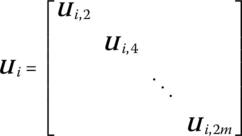
where
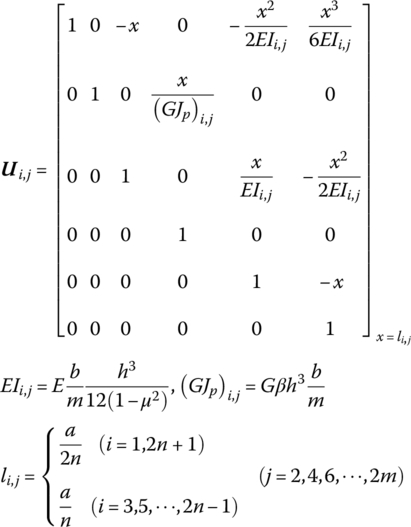
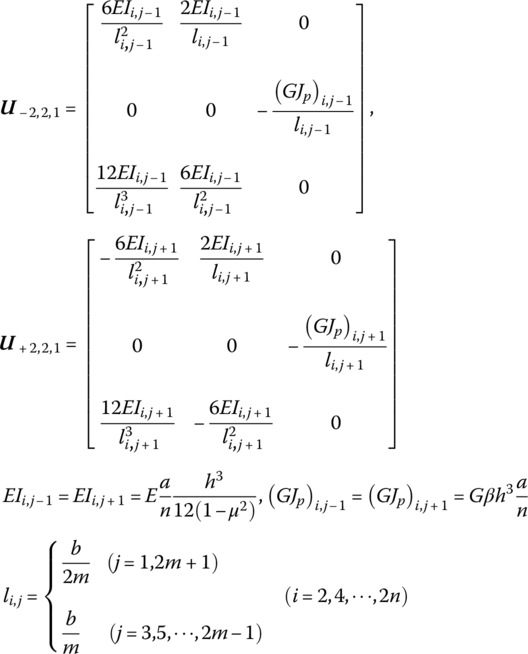
![]() is the transfer matrix of the single elastic beam, and (i, j), EIi,j, li,j, (GJp)i,j are the bending stiffness, length and torsional stiffness of beam (i, j) respectively. E is Young’s modulus, h is the thickness of the plate, μ is Poisson’s ratio, G is the shear elastic modulus and β is determined by the ratio of the length to width in the rectangle section,
is the transfer matrix of the single elastic beam, and (i, j), EIi,j, li,j, (GJp)i,j are the bending stiffness, length and torsional stiffness of beam (i, j) respectively. E is Young’s modulus, h is the thickness of the plate, μ is Poisson’s ratio, G is the shear elastic modulus and β is determined by the ratio of the length to width in the rectangle section, ![]() when the corresponding ratio is greater than 10 [245].
when the corresponding ratio is greater than 10 [245].
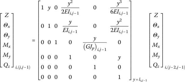
When ![]() , the strip elements in the ith column consist of m lumped masses and
, the strip elements in the ith column consist of m lumped masses and ![]() massless elastic beams in series sequentially along the y axis. The transfer equation of this strip element is similar to Equation (4.164), as follows
massless elastic beams in series sequentially along the y axis. The transfer equation of this strip element is similar to Equation (4.164), as follows
The transfer equation of a single lumped mass inside the network is the precondition of deriving Equation (4.167). The single lumped mass inside the network contains three input ends and one output end, and the transfer equation is derived as follows. The forces acting on the lumped mass are shown in Figure 4.21. According to the displacement continuous conditions and the force equilibrium of the lumped mass at the both input and output ends
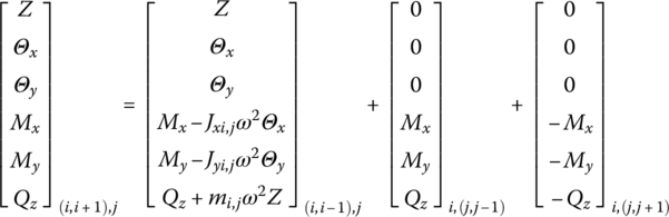
where
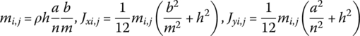
Figure 4.21 Force analysis of a lumped mass element.
mi,j is the mass of lumped mass (i, j), and Jxi,j and Jyi,j are the moments of inertia relative to the x and y axes, respectively.
Because of the transfer equation of beam ![]()
hence

Applying similar steps, the equations arising from the transfer equation of the beam element ![]() are
are
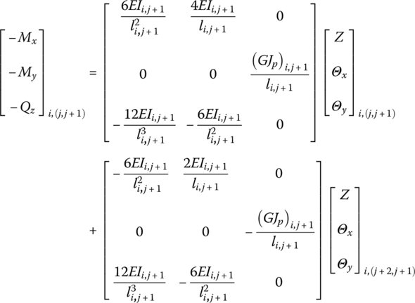
Considering the geometric relationship of each connection point and substituting each of the above equations into Equation (4.168), the transfer equation of a single lumped mass inside the network is
where

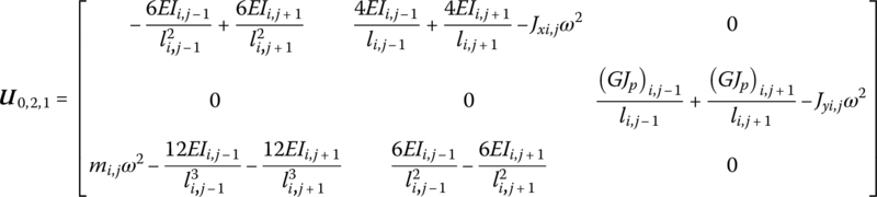
Equation (4.169) is called the transfer equation of single lumped mass inside the network. The transfer equation of the lumped mass on the edges, for instance ![]() or
or ![]() , includes the boundary condition at the boundary
, includes the boundary condition at the boundary ![]() or
or ![]() .
.
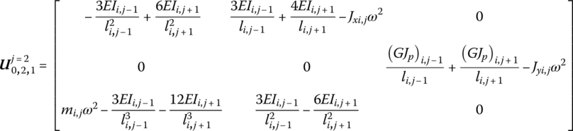
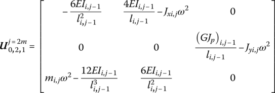
Using a similar method as used to derive Equation (4.169), at the boundary ![]() , namely
, namely ![]() , the transfer equation can be written as
, the transfer equation can be written as
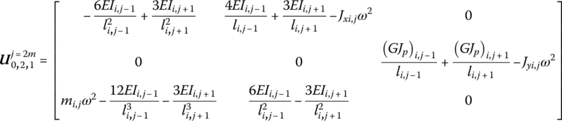
and at the boundary ![]() , when
, when ![]() , the transfer equation can be written as
, the transfer equation can be written as
where
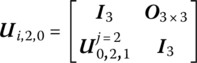
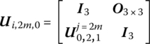
Submatrix ![]() in Equation (4.175) is given in Equation (4.171c). Submatrix
in Equation (4.175) is given in Equation (4.171c). Submatrix ![]() in Equation (4.176) is given in Equation (4.171a). However, to determine Ui,2,0 and Ui,2m,0 in Equations (4.175) and (4.176), the boundary conditions at
in Equation (4.176) is given in Equation (4.171a). However, to determine Ui,2,0 and Ui,2m,0 in Equations (4.175) and (4.176), the boundary conditions at ![]() and
and ![]() must be considered.
must be considered.
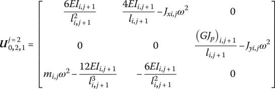
For instance, the boundary ![]() is simply supported, so the transfer equation of beam (i, 1) can be written as
is simply supported, so the transfer equation of beam (i, 1) can be written as
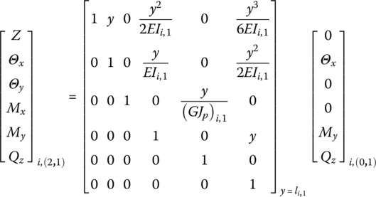
that is
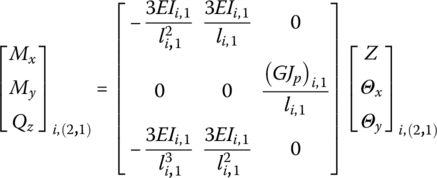
We obtain
If the boundary ![]() is also simply supported, then
is also simply supported, then
Similarly, Ui,2,0 and Ui,2m,0 in Equations (4.175) and (4.176) under other boundary conditions can be obtained:

If the boundaries of ![]() and
and ![]() are clamped, both
are clamped, both ![]() and
and ![]() can be determined by Equation (4.172a). If the boundaries of
can be determined by Equation (4.172a). If the boundaries of ![]() and
and ![]() are free,
are free, ![]() and
and ![]() are determined by both Equations (4.182) and (4.183):
are determined by both Equations (4.182) and (4.183):
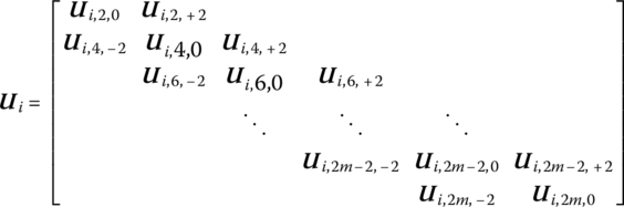
Therefore, the transfer matrix Ui in Equation (4.167) can be obtained from Equations (4.169), (4.173) and (4.174),
4.7.3 Boundary Conditions and Characteristic Equations
Equations (4.164) and (4.167) give rise to the overall transfer equation
Applying boundary conditions, the boundary state vectors Z0,1 and ![]() can be evaluated from Equation (4.185). For instance, assume the boundaries
can be evaluated from Equation (4.185). For instance, assume the boundaries ![]() and
and ![]() are both simply supported:
are both simply supported:

In other words, the ![]() th elements, 3m in total, in boundary state vectors Z0,1 and
th elements, 3m in total, in boundary state vectors Z0,1 and ![]() are zero. Therefore, the characteristic equations can be determined by substituting Equations (4.186) and (4.187) into Equation (4.185):
are zero. Therefore, the characteristic equations can be determined by substituting Equations (4.186) and (4.187) into Equation (4.185):
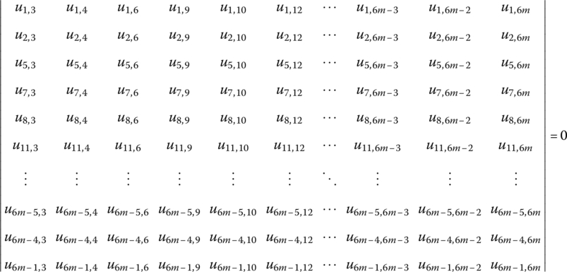
The eigenfrequencies of each order of the system can be obtained by solving the characteristic equations. The corresponding boundary state vectors Z0,1 and ![]() can be determined by substituting the eigenfrequencies of each order into Equation (4.185), and the eigenvectors which correspond to the eigenfrequencies can be obtained by using the transfer equations of each strip element.
can be determined by substituting the eigenfrequencies of each order into Equation (4.185), and the eigenvectors which correspond to the eigenfrequencies can be obtained by using the transfer equations of each strip element.
If ![]() and
and ![]() are clamped or free boundaries, the eigenfrequencies and eigenvectors in the relevant boundary conditions can be easily evaluated by re‐determining the boundary state vectors Z0,1 and
are clamped or free boundaries, the eigenfrequencies and eigenvectors in the relevant boundary conditions can be easily evaluated by re‐determining the boundary state vectors Z0,1 and ![]() in Equations (4.186) and (4.187) using the corresponding boundary conditions and substituting them into the overall transfer equation.
in Equations (4.186) and (4.187) using the corresponding boundary conditions and substituting them into the overall transfer equation.
4.7.4 Numerical Examples