
6
Transfer Matrix Method for Multi‐flexible‐body Systems
6.1 Introduction
The transfer matrix method for multi‐rigid‐body systems was introduced in Chapter 5. The translational and angular accelerations together with internal forces and moments are taken as new state variables instead of position coordinates in the original transfer matrix method for multibody systems (MSTMM). This results in totally different transfer matrices of elements and algorithms compared with the original MSTMM. The proposed method expands the advantages of the MSTMM by allowing more sophisticated numerical integration procedures to be used, such as the Runge–Kutta method: no global dynamics equations of the system are required, matrices have low order, setup of the global transfer equation is highly programmable, and solution allows high computational precision since linearization is not required anymore. The new method is simple, straightforward, efficient, practical and provides a powerful tool for multibody system dynamics (MSD).
The dynamics of a multi‐rigid‐flexible‐body system could also be solved by the transfer matrix method, in a way that is similar to dealing with a multi‐rigid‐body system. Hereafter, the way to study the dynamics of a multi‐rigid‐flexible‐body system by using the transfer matrix method is called the transfer matrix method for multi‐flexible‐body systems, which is introduced in this chapter.
The floating frame of reference formulation is used while modeling a flexible body, which satisfies the assumption of small deformation. Using the small deformation assumption and the modal superposition method, the partial dynamics equations of the flexible body can be discretized into ordinary differential equations about the generalized coordinates. Then we can proceed to the next step, that is, to deduce the transfer equation and the corresponding transfer matrix of the flexible body.
The translational and angular accelerations together with internal forces and moments are taken as new state variables for flexible bodies. Recall that the same state variables are used in the transfer matrix method for multi‐rigid‐body systems. However, the form of the transfer equations in the transfer matrix method for multi‐flexible‐body systems will be a little different from that of the transfer equations in the transfer matrix method for multi‐rigid‐body systems due to consideration of the deformation of the flexible bodies. There are two kinds of transfer equations in the transfer matrix method for multi‐flexible‐body systems: the first is used to assemble the overall transfer equations of the system and the second is used to solve the deformation acceleration of each flexible body. The division of the transfer equations of flexible bodies makes it much simpler to analyze a general multibody system which consists of rigid bodies and flexible bodies using the transfer matrix method for multibody systems.
6.2 State Vector, Transfer Equation and Transfer Matrix
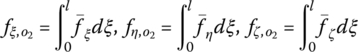
For simplicity, a chain multibody system is taken as an example to sketch the ideas of the transfer matrix method for multi‐flexible‐body systems. The new state vectors of the input and output ends of any flexible bodies and hinges moving in space are defined as
or
where
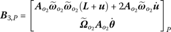
![]() , ÿ,
, ÿ, ![]() ,
, ![]() ,
, ![]() and
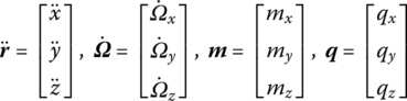
and ![]() are the absolute accelerations of the connection point with respect to the inertial reference system oxyz and the corresponding absolute angular accelerations in the directions of x, y and z, mx, my, mz,
are the absolute accelerations of the connection point with respect to the inertial reference system oxyz and the corresponding absolute angular accelerations in the directions of x, y and z, mx, my, mz, ![]() , qy and qz are the corresponding internal torques and internal forces in the same reference system, respectively, and
, qy and qz are the corresponding internal torques and internal forces in the same reference system, respectively, and ![]() ,
, ![]() ,
, ![]() and
and ![]() are the column vectors of absolute accelerations, absolute angular accelerations, internal torques and internal forces in oxyz, respectively.
are the column vectors of absolute accelerations, absolute angular accelerations, internal torques and internal forces in oxyz, respectively.
For a chain system moving in a plane, the new state vectors of the input ends and output ends of any flexible bodies and hinges are defined as
or
where

Then the dynamics equations of the jth flexible element can be assembled into two transfer equations
The transfer Equation (6.7) describes the transfer relationship between the state vectors at two ends of the jth element and the transfer Equation (6.8) is used to evaluate the deformation acceleration of the flexible body. Here, the matrix ![]() is the transfer matrix of the jth element which is known at time instant ti. Its order is always (13 × 13) for any dynamics of a chain multi‐rigid‐body system moving in space or (7 × 7) for any dynamics of a chain multi‐rigid‐body system moving in a plane.
is the transfer matrix of the jth element which is known at time instant ti. Its order is always (13 × 13) for any dynamics of a chain multi‐rigid‐body system moving in space or (7 × 7) for any dynamics of a chain multi‐rigid‐body system moving in a plane.
6.3 Overall Transfer Equation and Overall Transfer Matrix
According to Newton’s third law, the state vector of the output end of an inboard element is equal to the state vector of the input end of an outboard element for any two adjoining elements in a multibody system. The overall transfer equation and transfer matrix of the system, which relates the state vectors at the boundaries of the system, can therefore be assembled for any chain multibody system as follows:
It can be seen from the overall transfer equation and the overall transfer matrix that the order of the overall transfer matrix of the system is equal to the order of the transfer matrix of an element for a chain system, and it does not increase even if the degrees of freedom of the system increase. Irrespective of the size of a multibody system, the highest order of the overall transfer matrix is the same as the order of the transfer matrix of a single body, that is, (13 × 13) for the dynamics of a chain multibody system moving in space or (7 × 7) for the dynamics of a chain multibody system moving in a plane. The matrices involved in the new MSTMM are therefore always small, which greatly reduces the computational time and the memory storage requirement.
6.4 Transfer Matrix of a Planar Beam
A planar flexible beam is shown in Figure 6.1, where o2x2y2z2 is the floating frame of the flexible body and oxyz is the global inertial coordinate system. If there is no deformation of the flexible beam, the axis of the beam will coincide with o2x2 and the input point I of the beam will coincide with o2. Any point P on the beam is identified by its abscissa ![]() in o2x2y2z2, where the abscissa of the input point is 0, the mass center is ξC and the output point is l. l is also the length of the flexible beam.
in o2x2y2z2, where the abscissa of the input point is 0, the mass center is ξC and the output point is l. l is also the length of the flexible beam. ![]() and
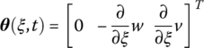
and ![]() are used to represent the distributed external forces acting on the flexible beam. u(ξ, t) and v(ξ, t) are the deformations of the beam along the directions of o2x2 and o2y2, respectively. The absolute accelerations, absolute angular accelerations, internal moments and internal forces of the input point or output point of the beam are denoted as
are used to represent the distributed external forces acting on the flexible beam. u(ξ, t) and v(ξ, t) are the deformations of the beam along the directions of o2x2 and o2y2, respectively. The absolute accelerations, absolute angular accelerations, internal moments and internal forces of the input point or output point of the beam are denoted as ![]() ,
, ![]() , mz,I(mz,O) and
, mz,I(mz,O) and ![]() , respectively, which are represented in oxyz. According to the sign conventions, the positive directions of
, respectively, which are represented in oxyz. According to the sign conventions, the positive directions of ![]() and mz,O coincide with the positive directions of the axes of oxyz, while the positive directions of
and mz,O coincide with the positive directions of the axes of oxyz, while the positive directions of ![]() and mz,I coincide with the negative direction of the axes of oxyz.
and mz,I coincide with the negative direction of the axes of oxyz.
Figure 6.1 A planar beam with large motion.
6.4.1 Deformation Mode of a Flexible Beam
The free vibration differential equations of a flexible beam are

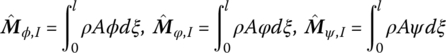
The inherent mode shapes and eigenvalues of the flexible beam along o2x2 and o2y2 are denoted by ϕ(ξ) and λϕ, φ(ξ) and λφ, respectively. The orders of ϕ(ξ) and φ(ξ) are noted as nϕ and nφ, respectively, the value of which depends on the convergence of the specific dynamical system. Let


It can be verified that ![]() ,
, ![]() ,
, ![]() and
and ![]() are all diagonal matrices and satisfy the following relationships
are all diagonal matrices and satisfy the following relationships
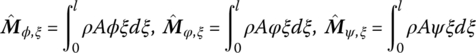
As a result of the couplings among the vibrations in different directions and the large motion of the beam, the following constant parameters are defined


6.4.2 Dynamics Equation of a Planar Beam
For an arbitrary point P on the axis of a flexible beam, the orientation angle, absolute angular velocity and the absolute angular acceleration are, respectively

The position vector from the origin of oxyz to point P is
where ![]() is the direction cosine matrix of o2x2y2z2 with respect to oxyz, which satisfies
is the direction cosine matrix of o2x2y2z2 with respect to oxyz, which satisfies
The absolute velocity and acceleration of point P can be easily obtained by differentiating Equation (6.19) with respect to time
The translational equation and the rotation equation of the beam, which makes up the dynamics equations governing the large motion of the beam, can be deduced based on the theorems of momentum and moment, respectively, as follows
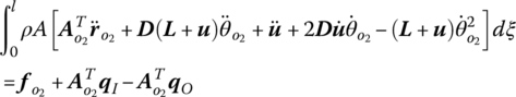

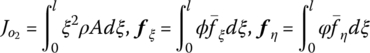
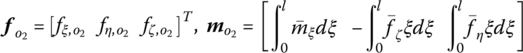
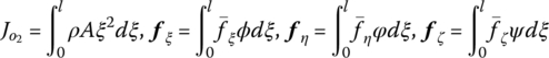
where


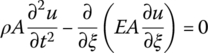
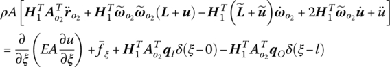
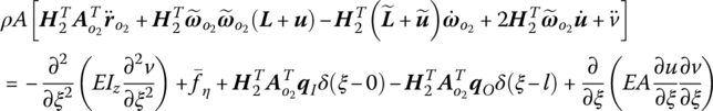
The dynamics equations governing the longitudinal vibration and the transverse vibration of the beam are, respectively
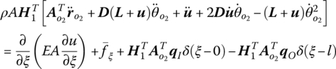

The last term of Equation (6.31) is used to take the effects of the axial force on the transverse vibration into consideration.
For an arbitrary point P on the axis of the flexible beam, we define
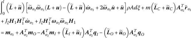
To carry out the next step, the deformation of the beam is expanded into the form of modal superposition. Substituting the discretized deformation into the dynamics equations of the beam described by partial differential equations, we can obtain the governing equations of the beam in the form of ordinary differential equations. The dynamics equations governing the large motion and the vibration of the beam are, respectively
where


6.4.3 Deduction of the Transfer Equation of a Planar Beam
The kinematics Equations (6.18) and (6.25) of the beam can be combined and rewritten in the following form
where
Then for the input and output points of the beam we have
Define the form of the state vector ![]() of the connecting points of the beam, including the input and output points, as
of the connecting points of the beam, including the input and output points, as
which can be rewritten simplified as
Combining Equations (6.33), (6.34), (6.47) and (6.48), the transfer equation of the planar beam can be obtained, namely
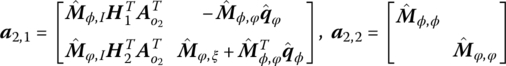
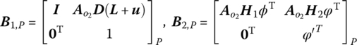
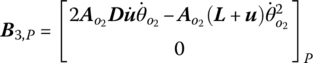
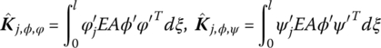
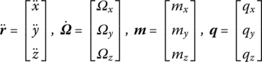
The corresponding transfer matrices are

where
6.5 Transfer Matrix of a Spatial Beam
A spatial flexible beam is shown in Figure 6.2, where o2x2y2z2 is the floating frame of the flexible body and oxyz is the global inertial coordinate system. If there is no deformation of the flexible beam, the axis of the beam will coincide with o2x2 and the input point I of the beam will coincide with o2. Any point P on the beam is identified by its abscissa ![]() in o2x2y2z2, where the abscissa of the input point is 0, the mass center is ξC and the output point is l. l is also the length of the flexible beam.
in o2x2y2z2, where the abscissa of the input point is 0, the mass center is ξC and the output point is l. l is also the length of the flexible beam. ![]() ,
, ![]() and
and ![]() are used to represent the distributed external forces acting on the flexible beam and u(ξ, t), v(ξ, t) and w(ξ, t) the deformations of the beam in the directions of o2x2, o2y2 and o2z2, respectively. The absolute accelerations, absolute angular accelerations, internal moments and internal forces of the input or output point of the beam are denoted by
are used to represent the distributed external forces acting on the flexible beam and u(ξ, t), v(ξ, t) and w(ξ, t) the deformations of the beam in the directions of o2x2, o2y2 and o2z2, respectively. The absolute accelerations, absolute angular accelerations, internal moments and internal forces of the input or output point of the beam are denoted by ![]() ,
, ![]() ,
, ![]() and
and ![]() , respectively, which are represented in oxyz. According to the sign convention, the positive directions of
, respectively, which are represented in oxyz. According to the sign convention, the positive directions of ![]() and
and ![]() coincide with the positive directions of the axes of oxyz, while the positive directions of
coincide with the positive directions of the axes of oxyz, while the positive directions of ![]() and
and ![]() coincide with the negative direction of the axes of oxyz.
coincide with the negative direction of the axes of oxyz.
Figure 6.2 A spatial beam with large motion.
6.5.1 Deformation Mode of a Flexible Beam
The free vibration differential equations of a flexible beam are

The inherent mode shapes and eigenvalues of the flexible beam along o2x2, o2y2 and o2z2 are denoted by ϕ(ξ) and λϕ, φ(ξ) and λφ, and ψ(ξ) and λψ, respectively. The orders of ϕ(ξ), φ(ξ) and ψ(ξ) are nϕ, nφ and nψ, respectively, the value of which depends on the convergence of the specific dynamical system. Let


It can be verified that ![]() ,
, ![]() ,
, ![]() ,
, ![]() ,
, ![]() and
and ![]() are all diagonal matrices that satisfy the following relationships
are all diagonal matrices that satisfy the following relationships
As a result of the couplings among the vibrations in different directions and the large motion of the beam, the following constant parameters are defined

6.5.2 Dynamics Equation of a Spatial Beam
For an arbitrary point P on the axis of a flexible beam, the rotation angle caused by the deformation of the beam is
which is represented in o2x2y2z2.
The direction cosine matrix, angular velocity and angular acceleration of the body fixed coordinate system of this point with respect to oxyz are, respectively
which are all represented in oxyz. ![]() is the direction cosine matrix of o2x2y2z2 with respect to oxyz.
is the direction cosine matrix of o2x2y2z2 with respect to oxyz.
The position vector from the origin of oxyz to point P is
where
The absolute velocity and acceleration of point P can be easily obtained by differentiating Equation (6.19) with respect to time
The translational equation and the rotation equation of the beam, which make up the dynamics equations governing the large motion of the beam, can be deduced based on the theorems of momentum and moment, respectively, as follows

where
The dynamics equations governing the longitudinal vibration and the transverse vibration of the beam are, respectively

The last term of Equation (6.31) is used to take the effects of the axial force on the transverse vibration into consideration. The same applies in Equation (6.85).
For an arbitrary point P on the axis of the flexible beam, we can define
To carry out the next step, the deformation of the beam is expanded into the form of modal superposition. Substituting the discretized deformation into the dynamics equations of the beam described by partial differential equations, we can obtain the governing equations of the beam in the form of ordinary differential equations. The dynamics equations governing the large motion and the vibration of the beam are, respectively
where


6.5.3 Deduction of the Transfer Equation of a Spatial Beam
The kinematics Equations (6.73) and (6.25) of the beam can be rewritten as
where
Then for the input and output points of the beam we have
The form of the state vector ![]() of the connecting points of the beam, including the input and output points, is defined as
of the connecting points of the beam, including the input and output points, is defined as
where
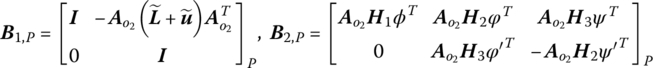
Combining Equations (6.33), (6.34), (6.47) and (6.48), the transfer equation of the spatial beam can be obtained, namely
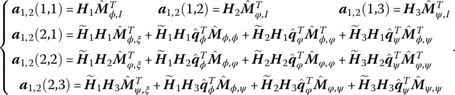
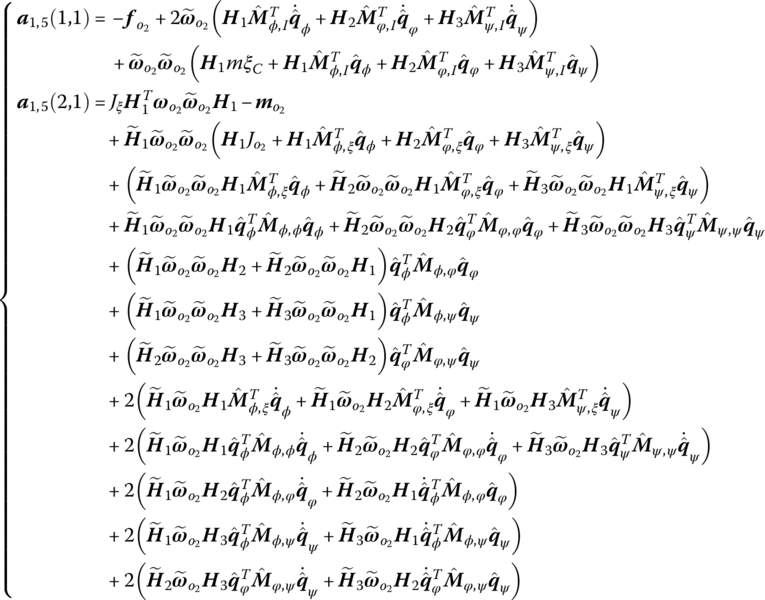
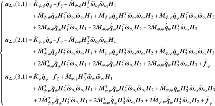
The corresponding transfer matrices are
where
6.6 Numerical Examples of Multi‐flexible‐body System Dynamics
To illustrate the procedure of how to solve the dynamics of the system using the transfer equations of elements, the dynamics of a hub–beam system and the dynamical system of a hub–beam system with a rigid body at the end of it are carried out.
6.6.1 Dynamics of a Hub–beam System
The hub–beam system is shown in Figure 6.3, where oxyz is the global inertial coordinate system. The hub is numbered 1 and the beam 2. The body fixed coordinate systems of the input and output points of the hub are shown in Figure 6.4 and those of the beam can be seen in Figure 6.2. The input point of the hub is connected to the global inertial coordinate system through a pin, which can rotate around the axis of oy, the beam is fixed on the hub, and its output end is free. An external moment M along the spin axis is applied to the hub as the driving force. The dynamic response of the system can be solved under zero initial conditions.
Figure 6.3 The hub–beam system.
Figure 6.4 The coordinates system of the hub.
The overall transfer equations of this system are
where ![]() and
and ![]() are the transfer matrices of elements 1 and 2, respectively.
are the transfer matrices of elements 1 and 2, respectively. ![]() is the state vector of the input point of element 1 and
is the state vector of the input point of element 1 and ![]() is the state vector of the output point of element 2. Equation (6.115) represents the attendant transfer equation of each flexible body element of the system, by which we can obtain the general acceleration of the deformation of each flexible body element after all the state vectors of the system are acquired.
is the state vector of the output point of element 2. Equation (6.115) represents the attendant transfer equation of each flexible body element of the system, by which we can obtain the general acceleration of the deformation of each flexible body element after all the state vectors of the system are acquired. ![]() and
and ![]() both belong to the state vectors of the boundaries of the system, which satisfy
both belong to the state vectors of the boundaries of the system, which satisfy
The state vectors of the boundaries of the system can be obtained by substituting the boundary conditions of Equations (6.116) and (6.117) into the overall transfer Equation (6.114) of the system, and then all the state vectors of the system can be determined using the transfer equation of each element of the system. Choosing the fourth‐order Runge–Kutta method, one of the numerical methods for ordinary differential equations, we can conduct the dynamical simulation of the system easily.
The physical parameters of the system are as follows. The length of beam is ![]() , the area of the cross‐section is
, the area of the cross‐section is ![]() , the moment of inertia of the cross‐section is
, the moment of inertia of the cross‐section is ![]() , the density of the material is
, the density of the material is ![]() , the elasticity modulus is
, the elasticity modulus is ![]() , the radius of the hub is
, the radius of the hub is ![]() , the mass of the hub is
, the mass of the hub is ![]() and the matrix of the moment of inertia of the hub is
and the matrix of the moment of inertia of the hub is ![]() .The external moment acting on the hub is given as shown in Figure 6.5. The responses of the rotational angular velocity of the hub, and the longitudinal and transversal deformations of the end of the beam are shown in Figures 6.6, 6.7 and 6.8, respectively.
.The external moment acting on the hub is given as shown in Figure 6.5. The responses of the rotational angular velocity of the hub, and the longitudinal and transversal deformations of the end of the beam are shown in Figures 6.6, 6.7 and 6.8, respectively.
Figure 6.5 The external moment acting on the hub.
Figure 6.6 The rotational angular velocity of the hub.
Figure 6.7 The longitudinal deformation of the end of the beam.
Figure 6.8 The deformation of the beam along o2z2.
6.6.2 Dynamics of a Hub‐beam System with a Rigid Body
The hub–beam system with a rigid body at the end is shown in Figure 6.9. The terminal rigid body is numbered 3, and the body fixed coordinate systems of its input and output points are shown in Figure 6.10. The rigid body is fixed on the beam, which is numbered 2. Just as in previous section, an external moment M along the spin axis is applied on the hub as the driving force. The dynamic response of the system can be solved under zero initial conditions.
Figure 6.9 A hub–beam system with a terminal rigid body.
Figure 6.10 The coordinates system of the terminal rigid body.
The overall transfer equations of the system are
where ![]() ,
, ![]() and
and ![]() are the transfer matrix of elements 1, 2 and 3, respectively.
are the transfer matrix of elements 1, 2 and 3, respectively. ![]() is the state vector of the input point of element 1 and
is the state vector of the input point of element 1 and ![]() is the state vector of the output point of element 3. The meaning of Equation (6.119) is the same as that of Equation (6.115).
is the state vector of the output point of element 3. The meaning of Equation (6.119) is the same as that of Equation (6.115). ![]() and
and ![]() both belong to the state vectors of the boundaries of the system, which satisfy
both belong to the state vectors of the boundaries of the system, which satisfy
The state vectors of the boundaries of the system can be obtained by substituting the boundary conditions of Equations (6.120) and (6.121) into the overall transfer Equation (6.118) of the system, and then all the state vectors of the system can be determined using the transfer equation of each element of the system.
It is assumed that the terminal rigid body is given with a mass of 0.2 kg and zero moment of inertia. All the other parameters are the same as those given in section 6.6.1. The responses of the rotational angular velocity of the hub and the transversal deformations of the end of the beam are shown in Figures 6.11 and 6.12, respectively.
Figure 6.11 The rotational angular velocity of the hub.
Figure 6.12 The deformation of the beam along o2z2.