
14
Dynamics of Shipboard Launch Systems
14.1 Introduction
Shipboard launch systems are essential ship‐borne weapons because of their rapid reaction, high firing rate, large allowance of ammunition, strong continuous fighting ability, difficult‐to‐intercept projectiles and high economic efficiency. These advantages make shipboard launch systems high‐efficiency weapons against marine and aerial targets, as well as targets on land. Shipboard launch systems are powerful in modern warfare and many destroyers are equipped with 127‐mm or 130‐mm shipboard launch systems. Any launch system can be regarded as a nonlinear, time‐variant multi‐rigid‐flexible‐body system. The nonlinear and time‐variant characteristics of shipboard launch systems include the time‐variant mass distribution and stiffness distribution caused by the large motion of the gun body and the projectile during the launching process, and collisions induced by the projectile–barrel gap.
In this chapter, we utilize discrete time transfer matrix method for multi‐rigid‐flexible‐body systems to solve some important problems in the launch dynamics of shipboard launch systems [112, 113].
14.2 Dynamics Model of Shipboard Launch Systems
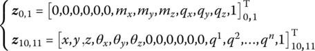
Shipboard launch systems are usually fixed on the deck of the ship, as shown in Figure 14.1. The Russian AK‐176 shipboard launch system is shown in Figure 14.2. Shipboard launch systems include a gun tube, breech, anti‐recoil devices, cradle, elevating mechanism, equilibrator, casemate, traversing mechanism, chassis, ramming mechanism, feeding mechanism, projectile hoist, barbette, ship body and so on. The launch dynamic model of a shipboard launch system is shown in Figure 14.3. The shipboard launch system can be cut at various connection points because of its component nature and divided into a number of mechanical parts. The ship's body and barbette form rigid body 2. The revolving part, not including the tipping part, is rigid body 4. The tipping part, not including the recoiling part, is rigid body 6. The breech and the part of a gun tube that slides on the cradle form rigid body 8. The part of the gun barrel that runs out of the cradle is an elastic beam, numbered 10. The anti‐recoil devices between the gun tube and the cradle are modeled as the massless sliding joint 7 and the spring‐damper between 8 and 6, and the mass of anti‐recoil devices is assigned to rigid bodies 8 and 6. The combination of the elevating mechanism and the equilibrator is regarded as the viscoelastic hinge 5 that joins 6 and 4. The masses of elevating mechanism and the equilibrator are merged into rigid bodies 6 and 4 in the theoretical analysis. The traversing mechanism is modeled by the viscoelastic joint 3 that connects bodies 4 and 2, whose mass is merged into rigid bodies 4 and 2. The interactive force of the seawater on the ship’s body is equivalent to the distributed‐elastic‐damping joint 1 [278]. Rigid body 8 and beam 10 are connected by a fixed joint 9. The parts below the seawater and the muzzle are regarded as the system boundaries and numbered 0 and 11, respectively. The launch dynamics model of a shipboard launch system has therefore developed as a nonlinear, time‐variant multi‐rigid‐flexible‐body system which moves under a powder gas drive. This system is composed of four rigid bodies and one elastic beam connected by a distributing elastic spring‐damping joint, two elastic joints, one sliding joint and one fixed joint.
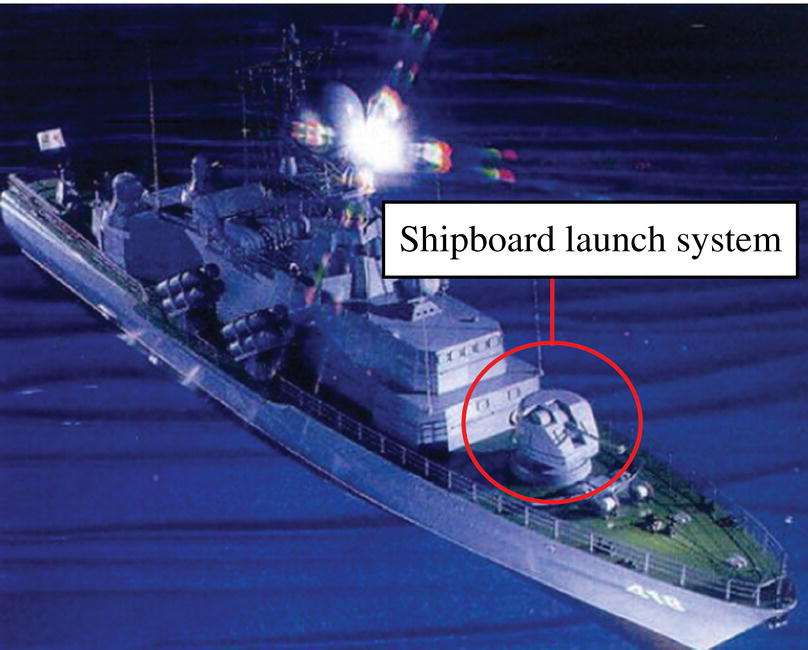
Figure 14.1 Russian Lightning class warship and AK‐176 shipboard launch system.
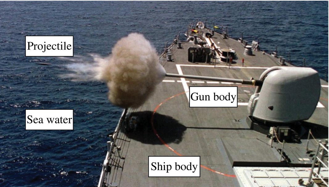
Figure 14.2 Russia AK‐176 shipboard launch system.
Figure 14.3 Launch dynamic model of a shipboard launch system.
When the projectile is moving in the gun tube, the main body of the projectile is regarded as a rigid body, and its elasticity effect is equivalent to the contacting elasticity between the rotating band, the bourrelet and the tube bore wall account. The factors of mass eccentricity and dynamic unbalance of the projectile, and the force between the projectile‐barrel and the powder gas thrust must be considered. Classical interior ballistic modeling has been used in the analysis.
14.3 State Vector, Transfer Equation and Transfer Matrix
Some state vectors, transfer equations and transfer matrices involved in the discrete time transfer matrix method for multibody systems (MSDTTMM) were introduced in Chapters 7 and 8. In this section, besides the above content, the special transfer matrices involved in the launch dynamics of shipboard launch systems will be introduced.
14.3.1 Distributed‐Elastic‐damping Foundation Equivalent to the Seawater
When the ship undergoes translational motion, the effect of seawater on the ship along the vertical orientation can be regarded as distributed elastic springs and dampers, but in the horizontal orientation there is only a damping effect. Likewise, only the damping effect is considered when the ship rotates around the vertical orientation. The effect of seawater on the ship can be modeled as the distributing spring and damper in the motion of ship rolling and pitching. Assuming that ![]() is the distributing elastic coefficient of vertical orientation, and
is the distributing elastic coefficient of vertical orientation, and ![]() and
and ![]() are distributing rotational elastic coefficients, we obtain
are distributing rotational elastic coefficients, we obtain
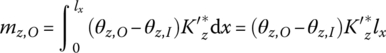
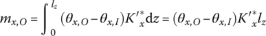
where lx and lz are the length and width of the ship’s bottom, respectively.
Considering the effect of damping, combining Equations (7.223), (14.2) and (14.3) yields
Rewriting the above equation gives
where
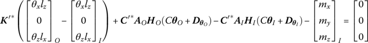
Combining Equations (14.1), (14.4) and (8.221) gives
Rearranging this yields
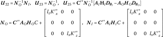
where
Thus the transfer equation of the distributed‐elastic‐damping foundation is
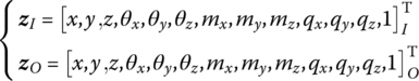
The state vectors are
The transfer matrix is
14.3.2 Sliding Joints
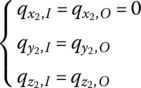
The gun tube moves on the cradle and mainly slides along the cradle axis under the action of anti‐recoil devices and the resultant interaction force between the gun tube and the projectile during the launching process. If the connection constraint between the gun tube and the cradle is regarded as a sliding joint, the action of the anti‐recoil devices is regarded as an external force and external moment between the gun tube and the cradle. The object shown in Figure 14.4 is a part of the gun tube. The interaction from the gun tube to the cradle is concentrated at point I and the interaction from the cradle to the gun tube is concentrated at point O. The input end I of the sliding joint is fixed on the cradle and the output end O of the sliding joint is fixed on the gun tube. We assume that points O and I coincide at the initial time and slide against each other. Let Ox2y2z2 be the body‐fixed coordinate system of the gun tube. Since the two rigid bodies only have relative linear motion along the x2 axis, the rotation angles of these two bodies are equal. The projections of the position vectors of the input and output ends on the y2 and z2 axes are equal. Thus, we have

Figure 14.4 Model of a sliding hinge.
If the friction and damping are eliminated we obtain
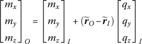
The position coordinates of output end O and input end I in the inertia coordinate system are
From Equations (14.12) and (14.13) we obtain
Projecting Equation (14.11) onto the inertia coordinate system yields
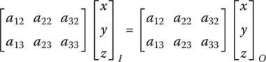
where (a11, a21, a31), (a12, a22, a32) and (a13, a23, a33) are elements of the transformation matrix A from the body‐fixed coordinate system to the inertia coordinate system of the gun tube.
Let ![]() , then from Equation (14.13) we obtain
, then from Equation (14.13) we obtain

Combining Equation (14.10) and Equations (14.14) to (14.17), and expressing the transformation matrix as the known function of previous time step, the transfer matrix of the sliding joint is
where

The elements of the transformation matrix ![]() are known as the functions of the previous time step.
are known as the functions of the previous time step.
14.4 Overall Transfer Equation of the System
According to the dynamic model of shipboard launch systems, the ship’s body and barbette 2 are regarded as rigid bodies under the action of distributing the basic elastic and damping effect. The revolving part, except for the tipping part, is regarded as rigid body 4, which has one input end and one output end. The tipping part, except for the recoil part, is regarded as rigid body 6, which has one input end and one output end. The breech and the gun tube slide on the cradle are regarded as rigid body 8, which has one input end and one output end. The remaining part of the gun tube is regarded as beam 10. The action of seawater on shipboard is equivalent to the distributed elastic damping joints 1, 3, and 5, 7 is a smooth elastic damping composite joint which can be regard as an elastic damping joint and a prismatic joint in series, whereas 9 is a fixed joint connecting the rigid body and the beam.
According to the launch dynamic model of the shipboard launch system, each element state vector of the system can be defined. z8,7 is the output end state vector of joint 7, which is located at a fixed point on the gun tube in contact with the cradle at the initial time.
The transfer matrix for distributing the basic elastic damping joint yields
From the transfer matrix equation of a rigid body with one input end and one output end, the transfer equations for the ship’s body, revolving body, cradle and breech can be obtained:
According to the transfer equation of an elastic damping joint, the transfer equations of elastic damping joints 3, 5 and 7 can be obtained:
According to the transfer matrix Equation (14.18) of a sliding joint, the transfer equation can be obtained:

The transfer matrix Equation (8.193) of a fixed joint from a rigid body to a beam yields the transfer equation from rigid body 8 to flexible gun tube 10, that is
According to the transfer matrix Equation (8.186) of a beam, the transfer equation of a flexible tube is
We obtain from the connection relationship of the shipboard launch system model:
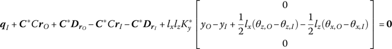
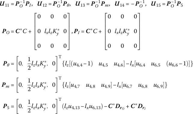
Combining Equations (14.67), (14.70) and (14.71), the transfer equation of the shipboard launch system is
where
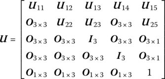
The overall transfer matrix of the shipboard launch system is
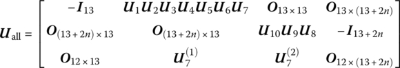
In conclusion, the overall transfer matrix of the shipboard launch system is obtained by combining the transfer matrices of the elements of the shipboard launch system. The process of establishing the overall transfer matrix of a system by using the transfer matrices of elements is just like the process of assembling the shipboard launch system by its parts. This is a simple and highly stable process.
14.5 Launch Dynamics Equation and Forces of the System
14.5.1 Force Analysis of the Shipboard Launch System
Only the external force is analyzed using the MSDTTMM. During the firing process, apart from the force of the projectile acting on the gun tube, the external force acting on the shipboard launch system involves total resistance to recoil, the powder gas’s force acting on the gun tube and the projectile’s force acting on the artillery. The interaction forces, such as the force between the cradle and the rotating body, the force between the rotating body and the ship’s body etc., are internal forces, internal moments and the corresponding damping forces. The expressions of the force and moment are made simple by using the MSDTTMM.
The recoil resistance force FR is
where FΦh is the recoil brake force, Ff is the recuperator force and F is the friction force of the sealing device. FT is the friction force of the cradle guiderail, mh is the mass of the recoiling parts and θ1 is the setting departure angle.
The resultant force of the recoil brake and recuperator can be expressed as
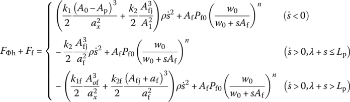
where s is the recoil distance, ![]() is the recoil velocity and
is the recoil velocity and ![]() is the working area of the recoil brake piston. DT is the inner diameter of the recoil cylinder and dT is the outer diameter of the recoil rod.
is the working area of the recoil brake piston. DT is the inner diameter of the recoil cylinder and dT is the outer diameter of the recoil rod. ![]() is the area of the throttling ring (dp is the inner diameter of the throttling ring) and
is the area of the throttling ring (dp is the inner diameter of the throttling ring) and ![]() is the working area of the return throttling device (d1 is the inner diameter of the recoil rod). A1 is the smallest cross‐section area of the branch and
is the working area of the return throttling device (d1 is the inner diameter of the recoil rod). A1 is the smallest cross‐section area of the branch and ![]() is the area of the liquid orifice corresponding to an arbitrary cross‐section of the throttling rod (
is the area of the liquid orifice corresponding to an arbitrary cross‐section of the throttling rod (![]() is an arbitrary cross‐section area of the throttling rod and dx is an arbitrary cross‐section diameter of the throttling rod). k1 is the coefficient of mainstream liquid resistance and k2 is the coefficient of a branch liquid resistance. ρ is the liquid density, k1,f is the coefficient of recuperating hydraulic pressure resistance and k2,f is the coefficient of the hydraulic pressure resistance of the return throttling device.
is an arbitrary cross‐section area of the throttling rod and dx is an arbitrary cross‐section diameter of the throttling rod). k1 is the coefficient of mainstream liquid resistance and k2 is the coefficient of a branch liquid resistance. ρ is the liquid density, k1,f is the coefficient of recuperating hydraulic pressure resistance and k2,f is the coefficient of the hydraulic pressure resistance of the return throttling device. ![]() is the working area of the recoil brake piston while recuperating, af is the area of the hole of the return throttling device and Pf0 is the initial gas pressure in the recuperator. Af is the working area of the recuperator piston, w0 is the initial gas volume in the recuperator, n is the polytrophic exponent and
is the working area of the recoil brake piston while recuperating, af is the area of the hole of the return throttling device and Pf0 is the initial gas pressure in the recuperator. Af is the working area of the recuperator piston, w0 is the initial gas volume in the recuperator, n is the polytrophic exponent and ![]() is the recoiling length,
is the recoiling length, ![]() .
.
The two friction forces are
where v is the sealing device friction coefficient and μ is the cradle guide‐rail friction coefficient.
When a projectile moves in the gun tube, the powder gas’s resultant force Fpt acting on the gun tube is made up of two parts: the breech pressure Ft and the axial component F2M of pressure on the chamber slope, that is
where
At is the area of the breech end, A is the cross‐section area of the rifled gun bore and Pt is the breech pressure.
The resultant force in the bore at the beginning of the gun ulterior period (the after‐effect period) is
where Pg is the mean pressure of powder gas in the bore at the beginning of the gun ulterior period, ω is the main charge mass, m is the projectile mass and φ1 is the coefficient of secondary work.
In the gun ulterior period, the process of powder gas outflow from the gun bore can be regarded as an ejection process of a semi‐closed round‐piped vessel with uniform cross‐section. If there is no muzzle brake, the resultant force in the bore during the ulterior period is
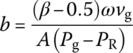
where b is the decay factor, tg is the time when the projectile flies out of the muzzle, tk is the termination time of the gun ulterior period, PR is the mean pressure of the powder gas in the gun bore at the end of the ulterior period, vg is the muzzle speed of the projectile and β is the coefficient of the powder gas effect.
When the pressure of the powder gas in the gun tube falls to ![]() , the gas exhaust ulterior period reaches its end. We have
, the gas exhaust ulterior period reaches its end. We have
that is
The formula for the resultant force in the bore Fpt is

The interaction forces between the projectile and the gun tube includes the contact force of the rotating band and the front bourrelet, and these are introduced in the following.
14.5.1.1 Engraving Force to Gun Tube
The value of the engraving resistance from the projectile to the gun tube ![]() is equal to the engraving resistance
is equal to the engraving resistance ![]() acting on the projectile, and its direction is along the tangential direction of bore axis pointing at muzzle. We have
acting on the projectile, and its direction is along the tangential direction of bore axis pointing at muzzle. We have
where
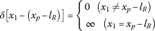
where x1 is the coordinate of an arbitrary point in the bore wall on the x axis in the gun tube coordinate system, xp is the coordinate of the projectile center of mass on the x axis in the gun tube coordinate system and lR is the distance between the center of the rotating band and the projectile center of mass. ![]() is the distance between the breech end and the center of the rotating band or the coordinate of the center of the rotating band on the x axis in the gun tube coordinate system, and
is the distance between the breech end and the center of the rotating band or the coordinate of the center of the rotating band on the x axis in the gun tube coordinate system, and ![]() is the Dirac function.
is the Dirac function.
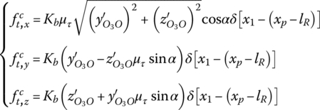
14.5.1.2 Driving Side Force and Moment to the Gun Tube
Under the action of the driving side force, the driving resistance ![]() and moment
and moment ![]() act on the projectile. Therefore, the driving side force
act on the projectile. Therefore, the driving side force ![]() and moment
and moment ![]() of the projectile to the gun tube are
of the projectile to the gun tube are

where C is the polar inertia moment of the projectile and ![]() is the angular velocity of the projectile.
is the angular velocity of the projectile.
14.5.1.3 Elastic Force and Moment between the Rotating Band and the Gun Tube
The applied forces caused by the elasticity and friction between the rotating band and the gun tube are
According to the Winkler elastic basic model, the elastic basic moment and the friction moment of the rotating band to the gun tube are

14.5.1.4 Effect of Front Bourrelet on the Gun Tube
The applied forces of the gun tube acting on the front bourrelet are
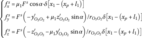
where l1 is the distance from the projectile center of mass to the front plane of the front bourrelet and ![]() is the radial displacement of O2 relative to the bore axis.
is the radial displacement of O2 relative to the bore axis.
For a curved tube, the inner surface of the gun bore does not have axial symmetry, that is, the up–down surface areas of the gun bore neutral plane will not equal each other any more. When the gun bore is filled with high‐pressure gas, the gas pressure makes the gun tube straight. This phenomenon is called the Bourdon effect and the force produced by the Bourdon effect is called the Bourdon force. The gun tube is not straight before firing. The Bourdon effect in a curving tube occurs when high‐pressure gas fills the gun tube, therefore the gun tube is loaded by the Bourdon force during the firing process.
The Bourdon force that is vertical to the axis of the gun tube is the distribution force acting on the gun tube behind the projectile, and it relates to the gas pressure in the gun bore, inner diameter and curvature of the gun tube. The formula of the Bourdon force acting on unit length is
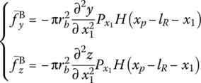
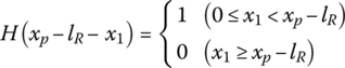
where x1 is the distance from an arbitrary point in the chamber to the breech end, ![]() is the gas pressure at x1, and
is the gas pressure at x1, and ![]() are the curvatures of the gun tube at x1. rb is the inner diameter of the gun tube,
are the curvatures of the gun tube at x1. rb is the inner diameter of the gun tube, ![]() is the Heaviside function and xp is the distance from the breech end to the projectile center of mass. lR is the distance from the center of the rotating band to the projectile center of mass, thus
is the Heaviside function and xp is the distance from the breech end to the projectile center of mass. lR is the distance from the center of the rotating band to the projectile center of mass, thus ![]() is the distance from the breech end to the center of the rotating band.
is the distance from the breech end to the center of the rotating band.
14.5.2 Force Analysis of the Projectile
In general, the rotating band is made of material that has good tractility. After launch ignition, the projectile makes the rotating band distort to embed into the rifling continually under high temperature and high‐pressure powder gas. The rifling here means “the cutting of spiral grooves on the inside of the barrel of the gun tube”. Generally, the process from ignition to the rotating band being completely embedded into the rifling is called the engraving process. The force status between the rotating band and the gun tube is complex during the engraving process. After the rotating band is embedded into the rifling, the twist angle of the rifling brings the driving side force between the rotating band and the rifling. Under the action of this force, projectile motion is affected by a rotating moment around the bore axis and the driving resistance force, which stops the projectile moving forward. When relative displacement arises between the centers of the rotating band and the bore axis because of the elasticity of the rotating band, the projectile is affected by elastic resilience. The rotating band and the gun bore are contacted via surfaces. When the geometry symmetric axis o1ξ of the projectile and the bore axis o0x0 deviate from each other, a basic restoring moment arises between the rotating band and the gun bore. During the launching process, some forces and moments between the rotating band and the gun bore have to be considered, that is, the engraving force and its moment, and the driving side force and its moment.
14.5.2.1 Engraving Resistance and its Moment
Engraving resistance can prevent a projectile moving forward and such a force is induced by the plasticity deformation of the rotating band when the rotating band embeds the rifling. It is expressed by ![]() and is related to the stress σn of the rotating band groove, the engraving contact area An, the coefficient of friction μn and the forcing cone angle ϕ, while it points at the breech along the bore axis. The matrix form of
and is related to the stress σn of the rotating band groove, the engraving contact area An, the coefficient of friction μn and the forcing cone angle ϕ, while it points at the breech along the bore axis. The matrix form of ![]() in the gun tube coordinate system o0x0y0z0 is
in the gun tube coordinate system o0x0y0z0 is
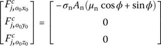
where An is the engraving contact area.
When engraving happens, the motion speed of the rotating band is not very high, therefore the coefficient of friction can be replaced by the static coefficient of friction. In general, the static coefficient of friction of copper to steel is ![]() . The stress σn of the rotating band groove can be computed with the following formula:
. The stress σn of the rotating band groove can be computed with the following formula:

For a copper rotating band, let ![]() and
and ![]() , thus
, thus ![]() and
and ![]() .
.
The expression for the engraving resistance moment ![]() in the body‐fixed coordinate system o1ξηζ is
in the body‐fixed coordinate system o1ξηζ is
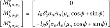
where lR is the distance from the center of the rotating band to the geometry center.
14.5.2.2 Driving Side Force and its Moment
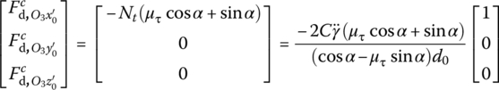
After the projectile was engraved into the rifling, under the action of the powder gas pressure and the driving side force of the rifling, the projectile moves straight along the bore axis and rotates at the same time. There are some contact and friction forces between the driving side of each rifling and the rotating band. Integrating this contact force along the gun bore axial direction intergral yields a total resultant force, denoted by Nt. Its effect can be divided into two parts, one is a driving resistance force ![]() , which prevents the projectile moving forward, the other is a moment
, which prevents the projectile moving forward, the other is a moment ![]() , which makes the projectile spin in the bore axis.
, which makes the projectile spin in the bore axis.
It can be verified that
where α is the twist angle of the rifling and μτ is the sliding coefficient of friction between the rotating band and the rifling.
The sliding coefficient of friction μτ between the copper rotating band and the rifling adopts a combing formula, that is
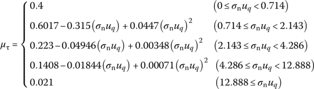
where the unit of σnuq is ![]() .
.
For a rifled gun, the twist angle of the gun tube rifling is a function of the projectile travel distance xq. For the combined twist rifling whose first part is increasing twist rifling and second part is uniform twist rifling, we have
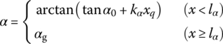
where lα is the position of the switch point of uniform twist rifling and increasing twist rifling, α0 is the initial twist angle of the rifling, αg is the twist angle of the muzzle rifling and ![]() .
.
From Equation (14.44), the relationship between the spin angle of the projectile and the displacement of the projectile xq is
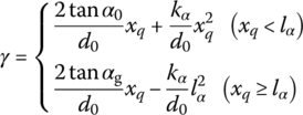
Differentiating Equation (14.45) yields

where uq and aq are the longitudinal velocity and longitudinal acceleration of the projectile relative to the gun bore, respectively.
The driving resistance force ![]() in the gun tube coordinate system
in the gun tube coordinate system ![]() can be written in matrix form
can be written in matrix form
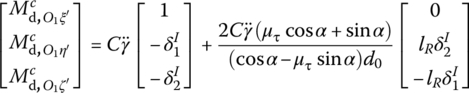
The driving resistance moment ![]() in the body‐fixed coordinate system O1ξ′η′ζ′ can also be written in matrix form
in the body‐fixed coordinate system O1ξ′η′ζ′ can also be written in matrix form
14.5.3 Launch Dynamics Equation of a Projectile
In the 1980s, the general motion differential equation of a projectile in a gun tube was developed by Marting, which brought research into projectile motion in a gun tube into a new phase. One weakness of Marting’s model is that it does not consider the dynamic unbalance of the projectile and dealing with the mass eccentricity of the projectile is not reasonable enough, but these two factors are very important in the study of launch dynamics. To address this, the authors made an essential improvement to Marting’s model and developed a uniform form of the dynamics equation of nonsymmetrical projectile motion in a gun tube and the ulterior period.
Considering the effect of the weight of the projectile in the bore, the contact force between the rotating band and gun bore, the air pressure of the powder gas and the contact force between the bourrelet and the gun tube and the corresponding moment, the dynamic equations of a nonsymmetrical projectile undergoing general motion in an increasingly twisted rifling gun tube are
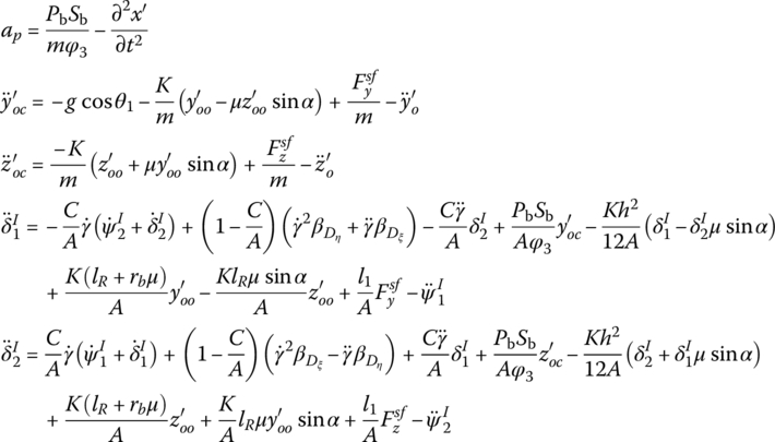
where ![]() and
and ![]() are the vertical and lateral displacements of the center of mass of the projectile relative to the gun tube coordinate system
are the vertical and lateral displacements of the center of mass of the projectile relative to the gun tube coordinate system ![]() ,, respectively.
,, respectively. ![]() is the acceleration of the center of mass of the projectile relative to the gun tube,
is the acceleration of the center of mass of the projectile relative to the gun tube, ![]() and
and ![]() are the pitch and revolution angles, respectively, formed by the misalignment of the tangent line of tube and projectile axes, and γ is the rotation angle of the projectile in the gun tube. Pb is the pressure of the projectile base, Sb is the area of the projectile base and m is the mass of the projectile. φ3 is the coefficient of second work, θ1 is the setting fire angle of the artillery and g is the acceleration due to gravity.
are the pitch and revolution angles, respectively, formed by the misalignment of the tangent line of tube and projectile axes, and γ is the rotation angle of the projectile in the gun tube. Pb is the pressure of the projectile base, Sb is the area of the projectile base and m is the mass of the projectile. φ3 is the coefficient of second work, θ1 is the setting fire angle of the artillery and g is the acceleration due to gravity. ![]() is the equivalence stiffness coefficient when the projectile contacts the bore wall, h is the width of the rotating band and rb is the radius of the projectile bourrelet. μ is the coefficient of friction between the rotating band and the bore wall, α is the rifling twist angle and A is the equator rotation inertia of the projectile. C is the polar inertia moment, lR is the distance from the centroid to the center of the rotating band and l1 is the distance from the center of mass of the projectile to the front plane of the bourrelet.
is the equivalence stiffness coefficient when the projectile contacts the bore wall, h is the width of the rotating band and rb is the radius of the projectile bourrelet. μ is the coefficient of friction between the rotating band and the bore wall, α is the rifling twist angle and A is the equator rotation inertia of the projectile. C is the polar inertia moment, lR is the distance from the centroid to the center of the rotating band and l1 is the distance from the center of mass of the projectile to the front plane of the bourrelet. ![]() is the recoiling acceleration of the gun tube and x is the distance from the rotating band to the beginning of the rifling in the equation of the spin angle. The dynamic unbalance of the projectile is
is the recoiling acceleration of the gun tube and x is the distance from the rotating band to the beginning of the rifling in the equation of the spin angle. The dynamic unbalance of the projectile is ![]() , where
, where ![]() is the projection of the dynamic unbalance on the η axis of the body‐fixed coordinate system and
is the projection of the dynamic unbalance on the η axis of the body‐fixed coordinate system and ![]() is the projection of the dynamic unbalance on the ξ axis of the body‐fixed coordinate system. The mass eccentricity of the projectile is
is the projection of the dynamic unbalance on the ξ axis of the body‐fixed coordinate system. The mass eccentricity of the projectile is ![]() , where
, where ![]() is the projection of the mass eccentricity on the η axis of the body‐fixed coordinate system and
is the projection of the mass eccentricity on the η axis of the body‐fixed coordinate system and ![]() is the projection of the mass eccentricity on the ξ axis of the body‐fixed coordinate system.
is the projection of the mass eccentricity on the ξ axis of the body‐fixed coordinate system. ![]() and
and ![]() are the vertical and lateral displacements of the center of mass of the projectile relative to the aiming line, respectively, and
are the vertical and lateral displacements of the center of mass of the projectile relative to the aiming line, respectively, and ![]() and
and ![]() are the vertical and lateral components of the angle between the tangent of the tube axis and the line of sight. Differentiating twice with respect to time yields
are the vertical and lateral components of the angle between the tangent of the tube axis and the line of sight. Differentiating twice with respect to time yields
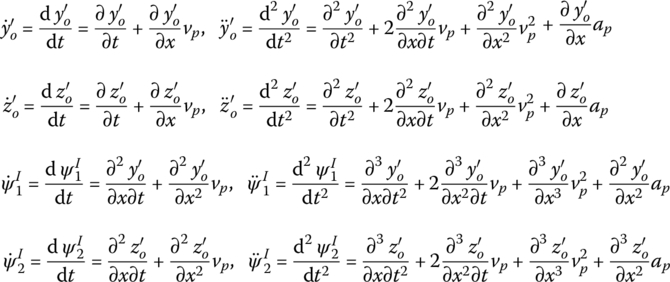
![]() and
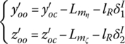
and ![]() are the vertical and lateral displacements of the center of the rotating band relative to the gun tube coordinate system
are the vertical and lateral displacements of the center of the rotating band relative to the gun tube coordinate system ![]() ,, respectively, that is
,, respectively, that is
Fsf is the contact force between the bourrelet and the bore, including collision and friction forces, that is
where
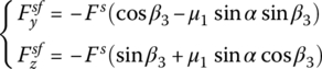
μ1 is the coefficient of friction between the bourrelet and the bore.
14.5.4 Equations of Classical Interior Ballistics
Classical interior ballistics theory has been used widely and can satisfy engineering requirements in many respects because it is a simple model on a small computational scale. The basic assumptions of classical interior ballistics are:
- The propellant bed burns at the same time and the initial pressure is the ignition pressure.
- The firing gas keeps the same components, and the physical and chemical performance parameters are all constant.
- Propellant burning obeys geometric burning law and exponential burning rate law, and the firing gas obeys the Nobel–Abel equation.
- The gas pressure in the gun tube obeys the Lagrange assumption.
The equations of interior ballistics are
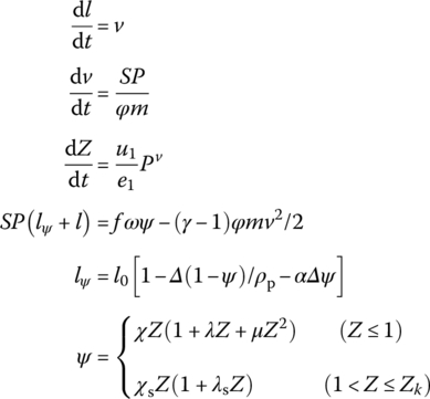
where l is the projectile travel distance, v is the velocity of the projectile and S is the area of the projectile base. m is the mass of the projectile, φ is the coefficient of second work and Z is the relative burning thickness of the propellant. e1, u1 and ν are half thickness, burning rate coefficient and burning rate exponent of propellant, respectively. P is the average pressure in the gun tube, ψ is the relative burning volume of the propellant and lψ is the chamber volume‐to‐bore area ratio. ω is the charge mass, l0 is the length of the powder chamber and α is the volume of powder gas. Δ is the loading density and ρp is the propellant solid density. χ, λ, μ, χs and λs are the shape characteristic parameters of the powder, while γ is the adiabatic exponent of the powder gas.
The pressure of the projectile base Pb is
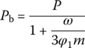
where W0 is the chamber volume, φ1 is the coefficient of resistance and ![]() .
.
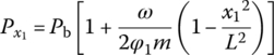
The distribution of gas pressure in the gun tube is
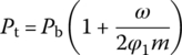
The breech pressure is
14.6 Solution of Shipboard Launch System Motion
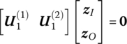
Substituting the system boundary conditions
into Equation (14.33), the motion of the shipboard launch system can be obtained. Thus, Equation (14.33) can be rewritten as
where ![]() is the residue column matrix after removing the zero state variables and 1 from the overall boundary state vector
is the residue column matrix after removing the zero state variables and 1 from the overall boundary state vector ![]() , and
, and ![]() is a matrix with (36 + 2n) order obtained from
is a matrix with (36 + 2n) order obtained from ![]() after the columns 1–6, 13, 26, 39, 46–51 and 52 + 2n, and rows 13 and 26 + 2n have been deleted.
after the columns 1–6, 13, 26, 39, 46–51 and 52 + 2n, and rows 13 and 26 + 2n have been deleted. ![]() is a column matrix obtained from adding columns 13, 26, 39 and 52 + 2n of
is a column matrix obtained from adding columns 13, 26, 39 and 52 + 2n of ![]() and then deleting rows 13 and 26 + 2n.
and then deleting rows 13 and 26 + 2n.
Thus, the matrix order involved in solving the dynamics of a complex shipboard launch MRFS by the MSTMM is low. The order of the transfer matrix of the system is 36 + 2n, but the degrees of freedom of a discrete system in a hybrid system are 24. The matrix order is much smaller than the matrix order ![]() obtained by ordinary methods, therefore the computational efficiency is very high.
obtained by ordinary methods, therefore the computational efficiency is very high.
![]() is obtained by solving the linear algebraic Equations (14.75), consequently
is obtained by solving the linear algebraic Equations (14.75), consequently ![]() is determined. The state vectors of any of the connection points can be determined by using the transfer equations of the elements, and the system motion can be obtained.
is determined. The state vectors of any of the connection points can be determined by using the transfer equations of the elements, and the system motion can be obtained.
The algorithm for solving the motion of a shipboard launch system is as follows:
- Confirm the initial conditions and boundary conditions of the system: let
 .
. - Obtain the values of
 on the various element joints using the linearization method.
 - Let the motion parameters of the system at time ti be the initial values, then the motion parameters of the projectile, the resultant force of the gun bore and the applied force of the projectile barrel are solved from the equations of the launch dynamics of the projectile (Equation (14.49)) and equations of interior ballistics (Equation (14.54)), and the resistance to recoil is solved from Equation (14.20).
- Compute the transfer matrix of the element and the overall transfer equation of the system by regarding the resultant force of the gun bore, the applied force of projectile‐barrel and the resistance to recoil as external forces.
- Compute the unknown quantities of the boundary state vectors using boundary conditions and the overall transfer equation of the system.
- Compute the state vectors of the connection point at time
 using the transfer equations of the elements.
 - Compute the position coordinates and attitude angles, and the corresponding velocities and accelerations using the state vector at
 .
. - Let
 , treat the computational result of step (7) as the initial conditions, and return to step (2) until the time required for complete analysis.
In conclusion, it is simple, efficient and highly programmable to solve the dynamics response of a complex shipboard launch the MRFS by using the MSDTTMM.
14.7 Dynamics Simulation of the System and its Test Verifying
14.7.1 Launch Dynamics Simulation System for a Shipboard Launch System
The numerical simulation system of the launch dynamics of the shipboard launch system is established based on the MSDTTMM. The launch dynamics process of a large‐caliber shipboard launch system with zero angle of elevation and zero angle of azimuth is numerically simulated. The vibration characteristics, rule of motion and initial disturbance of the projectile in the gun bore and the dynamic response of artillery are obtained. A related experiment is used to verify the simulation results. Some computation and experiment results are as follows.
14.7.2 Dynamics Simulation and Test Verifying for a Shipboard Launch System
The simulation results of the dynamic response of a shipboard launch system obtained by the launch dynamics simulation system for shipboard launch systems, as well as the corresponding experiment results, are shown in Figures 14.5–14.12. The simulation results for the muzzle position coordinate along the x axis are shown in Figure 14.5 and the simulation results for the time‐history of resistance to recoil are shown in Figure 14.6. Figures 14.7 and 14.8 show the simulation results of the time‐history of the muzzle position coordinate along the y and z axes, respectively. Figures 14.9 and 14.10 show the time history of the muzzle speed along the y and z axes, respectively. Figures 14.11 and 14.12 are plots of the simulation and experiment results for the lateral and vertical deflection angles of the muzzle. These figures show that the numerical simulation of launch dynamics for the shipboard launch system is in good agreement with the experiment results.
Figure 14.5 Muzzle position coordinate along the x axis.
Figure 14.6 Time history of recoil.

Figure 14.7 Muzzle position coordinate along the y axis.
Figure 14.8 Muzzle position coordinate along the z axis.
Figure 14.9 Muzzle speed along the y axis.
Figure 14.10 Muzzle speed along the z axis.
Figure 14.11 Simulation and experiment results of the lateral deflection angle of the muzzle.
Figure 14.12 Simulation and experiment results of the vertical deflection angle of the muzzle.
14.7.3 Launch Dynamic Simulation Result for a Projectile
The launch dynamic simulation results for a projectile obtained using the numerical simulation system of the launch dynamics of the shipboard launch system are shown in Figures 14.13–14.24. These figures show the time histories of the longitudinal displacement (Figure 14.13), the longitudinal velocity (Figure 14.14), the longitudinal acceleration (Figure 14.15) and the transverse displacement of the projectile (Figure 14.16), the collision force of the projectile‐barrel (Figure 14.17), the transverse speed of the mass centre of the projectile (Figure 14.18), and the lateral and vertical swing angles of the projectile axis (Figures 14.19 and 14.20, respectively). The lateral and vertical swing angular speeds of the projectile axis are shown in Figures 14.21 and 14.22, respectively. The time histories of the yaw angle and the mass center trajectory of the projectile are presented in Figures 14.23 and 14.24, respectively.
Figure 14.13 Longitudinal displacement.
Figure 14.14 Longitudinal velocity.
Figure 14.15 Longitudinal acceleration.
Figure 14.16 Transverse displacement.

Figure 14.17 Collision force of the projectile‐barrel.

Figure 14.18 Transverse velocity of the center of mass of the projectile.
Figure 14.19 Lateral swing angle of the projectile axis.
Figure 14.20 Vertical swing angle of the projectile axis.
Figure 14.21 Lateral swing angular velocity.
Figure 14.22 Vertical swing angular velocity.
Figure 14.23 Track of yaw angle of the projectile axis.
Figure 14.24 Track of the center of mass of the projectile.
14.7.4 Simulation and Test Verifying of Eigenfrequencies
The vibration characteristics of a large‐caliber shipboard launch system when the angle of elevation and the angle of azimuth are both zero are numerically simulated using the launch dynamics numerical simulation system for a shipboard launch system. A modal experiment is carried out, and the modal parameters of the shipboard launch system are obtained. The simulation and experiment results of the first 16 order eigenfrequencies are shown in Table 14.1. It can be seen that the numerical simulations and the experiment results are in good agreement, which validates the simulation results.
Table 14.1 Simulation and experiment results of eigenfrequencies
| Modal order, k | ωk/(rad/s) | Relative error/% | Modal order, k | ωk/(rad/s) | Relative error/% | ||
| Simulation | Experiment | Simulation | Experiment | ||||
| 1 | 6.3 | 6.26 | 1.27 | 9 | 26.9 | — | — |
| 2 | 7.6 | — | — | 10 | 32.1 | — | — |
| 3 | 11.3 | 11.24 | 0.85 | 11 | 34.6 | 36.86 | –6.13 |
| 4 | 11.4 | 11.25 | 1.7 | 12 | 38.8 | 41.12 | –5.49 |
| 5 | 15.5 | — | — | 13 | 43.4 | 42.41 | 2.33 |
| 6 | 18.9 | — | — | 14 | 64.0 | 60.51 | 5.89 |
| 7 | 20.7 | 21.32 | –2.61 | 15 | 65.1 | 67.77 | –3.92 |
| 8 | 26.1 | — | — | 16 | 74.4 | 74.35 | 0.08 |