
12
Dynamics of Multiple Launch Rocket Systems
12.1 Introduction
As a practical example in important engineering applications of the linear MSTMM, this chapter solves the difficult problem in launch dynamics of MLRSs using the MSTMM.
MLRSs with 40 launch tubes are the best equipped among MLRSs in the world today, for example the Russian БM‐21 type MLRS, shown in Figure 12.1. The number of launchers for an MLRS may be just a few or up to 40, and all the rockets can be launched in one volley in a few seconds, forming a glomerate assaulting strike. As a powerful oppressive weapon in modern war, MLRSs have received enormous attention from every powerful military country for their high speed, high power, violent firepower, long range, high mobility, ability to generate high‐density firepower in a short time, and many other tactical advantages. With the changing features of modern war and the development of new technologies, the status and function of MLRSs are more and more important. How can their firing precision be predicted? How can dynamic performance be guaranteed by dynamic design? How can rocket consumption in MLRS testing be decreased while still guaranteeing the quality of the test? To address these problems in the development, production and testing of MLRSs, it is necessary to solve the theory and technology issues that influence them. These issues have been given attention at home and abroad, for example the computation of vibration characteristics, the orthogonality of eigenvectors and the exact analysis of the dynamic response. Prediction of the launch dynamics of MLRSs requires an understanding of the acting forces, motion law and control processes during the launching of MLRSs and provides tools for scientific evaluation and improving the performance of MLRSs. The MSTMM is a powerful tool for studying the launch dynamics of MLRSs. The function of MLRS launch dynamics is that through studying the theory, simulation and testing of launch and flight dynamics of MLRSs from the point of view of a weapons system, and optimizing the total parameters of the system, it provides method and means for the dynamic design and performance evaluation of weapons. By studying the acting force and motion law of MLRSs under various disturbance factors, searching the computational method, measurement means and influence factors of initial disturbance and dynamic performance, establishing the quantitative relation between the total parameters of weapons and the initial disturbance and dynamic performance, and providing methods and technology means for the dynamic design and scientific evaluation of MLRS, the dynamic performance and combat ability of weapons can be improved, and the corresponding research period can be shortened. Improving production efficiency, decreasing rocket consumption in tests and increasing economic benefit can be realized by further decreasing the ball firing test.
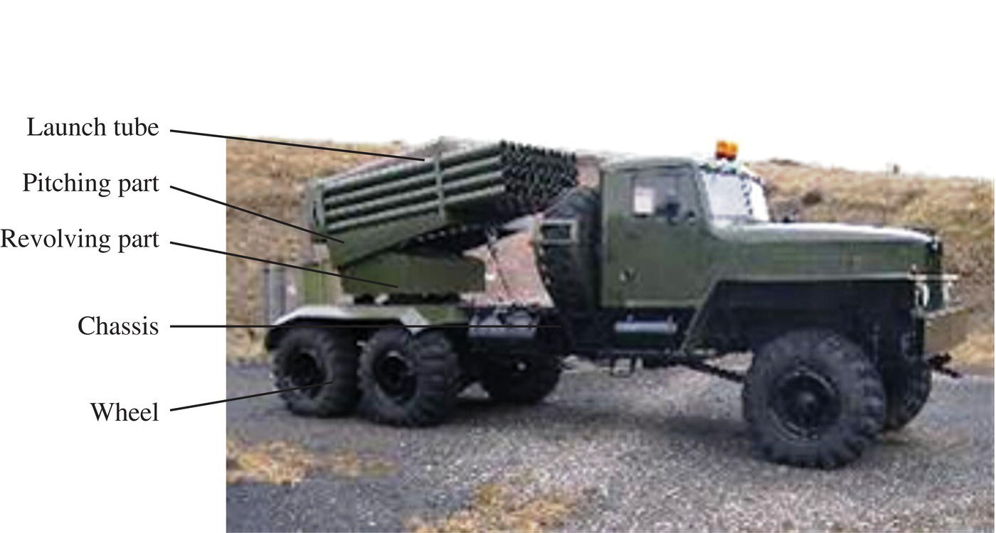
Figure 12.1 An MLRS with 40 launch tubes (Russia).
From the viewpoint of large system dynamics, including rockets, guns, propellants and the launch environment, the theory of MLRS launch dynamics is established in this chapter based on the MSTMM, where the process of MLRSs from ignition to the level point is studied. The difficult computation problem of the vibration characteristics of a multi‐rigid‐flexible‐body system (MRFS) for MLRSs is solved. The vibration characteristics of MLRSs and their variation with a change in the number of rockets on the launching equipment are obtained conveniently using the MSTMM. The exact analysis for the dynamic response of an MRFS for an MLRS is realized using the orthogonality theory of augmented eigenvectors established by authors, and the quantitative relation between the system performance of MLRSs and the firing sequence and firing interval is achieved. The two great practical applications of MLRS launch dynamics based on the MSTMM are also introduced in this chapter [87–101].
- A new test technology for MLRSs, with low rocket consumption under equivalent initial disturbance, is established, which solves the difficult problem for strong military countries of decreasing rocket consumption in MLRS tests. This technology has been used in the approval tests of several MLRSs in the National High‐Tech Project, with rocket consumption being decreased by 50–86%.
- The launch technology for MLRSs with low initial disturbance and high firing precision is established, which improves the firing precision and combat ability of several MLRSs of the National High‐Tech Project.
12.2 Launch Dynamics Model of the System and its Topology
MLRSs are used in almost all branches of the armed services, and the carrier vehicle can be an airplane, warship, ground vehicle and so on. In this chapter, an MLRS with 40 launch tubes carried by a ground vehicle is taken as an example to sketch the procedure of the study of the dynamics of the MLRS. This version is most often used, while the structures of the MLRS mounted on the other kinds of carrier vehicles are relatively much simpler than this case and their dynamics could be researched in a similar way. Firing precision includes firing accuracy and firing dispersion. The firing accuracy can be indicated from the deviation between the center of projectile scattering and the aiming point, which is determined by the characteristics of the weapon system itself, and can be corrected theoretically through many firings. The firing dispersion is used to express the scattering degree of projectiles with respect to the center of projectile scattering, and is usually denoted by E. The disturbance factors of rocket motion are divided into two kinds, random and deterministic. Random factors cannot be predefined, for example wind, initial disturbance, thrust malalignment, mass distribution unbalance, the deviation of the firing interval, the randomness of the MLRS vibration characteristics and so on. Deterministic factors can be predefined, for example the average deviation of air temperature and pressure, the weight deviation of the rocket, the loading position of the rocket, the firing sequence and so on. The influence of deterministic disturbance factors can be eliminated through ballistic correction theory [133], but the influence of random disturbance factors cannot be eliminated. The study of the change in initial disturbance and trajectory caused by various factors can provide a theoretic foundation and technology tool to evaluate and control firing precision.
The launch and free flight process of a rocket from firing and flying to impacting the target is divided into four phases.
- Locking phase: from the moment the rocket engine is fired to the moment the rocket begins to move. In this period, the rocket gun begins to move under the action of rocket propulsion, but it can only move longitudinally relative to the launch tube because of the locking mechanism.
- Moving in the launch tube: from the moment the rocket begins to move when it breaks loose from the locking mechanism under the action of rocket propulsion to the moment the rear bourrelet of the rocket leaves the launch tube. During this period, the motion of the rocket is restricted by the launch tube, leading to the mutual influence between the vibration of the rocket launcher and rocket motion. This, in addition to the gap between the bourrelet of rocket and launch tube, makes the rocket motion in launch tube very complex.
- Power phase: from the moment that the rear bourrelet of the rocket leaves the muzzle of the launch tube to the time that the fuel of the rocket engine burns out. In this period, the motion of the rocket is accelerated and the speed usually reaches a maximum when the fuel of the rocket engine burns out.
- Power‐off phase: from the moment that the fuel of the rocket engine burns out to the time that the rocket impacts the target, in which the rocket moves further with inertia due to its kinetic energy. Aerodynamics and gravity decrease the rocket velocity gradually during the climb phase, but the rocket velocity may increase during the fall phase.
Strictly speaking, the components of MLRSs are nonlinear elastic bodies in the launch process, and the dynamics model of a weapons system is a complex nonlinear elastic system with large rocket motion. Such engineering problems with complex models are impossible to solve even using today’s highly developed computation technology and mechanic theory, and in fact it is not necessary to regard them as complete elastic body models in engineering problems. As with most mechanism systems, the principle of engineering modeling is to simplify the model as much as possible and reduce the computation scale under the precondition of satisfying the engineering precision. That is to say, if the precision meets the engineering requirement, the component should be regarded as a simple lumped mass or rigid body. The component must be regarded as an elastic body if the precision does not meet the requirement when it is regarded as a lumped mass or rigid body, for example if it has been validated by tests that the stiffness of the MLRS launch tube has an obvious influence on its firing dispersion [249].
The components of MLRSs can be regarded as a lumped mass, rigid body, elastic beam, rotary spring, spring, damper and other mechanics elements according to their natural properties. The launch dynamics model of MLRSs with 40 launch tubes that is most often used around the world today is shown in Figure 12.2. The pitching part defined here does not include the fired rockets and the launch tube that loads the launching rocket, the gyration part defined here does not include the pitching part, the vehicle chassis excluding the wheels is called the vehicle, the trail of the launch tube excluding the newly launched rocket is called the launch tube trail, and each of these is regarded as a rigid body with 6 degrees of freedom (DOFs). The six wheels are regarded as a lumped mass with 3 DOFs. The launch tube defined here does not include the newly launched rocket (omitting the launch tube trail), and is regarded as an elastic beam moving in space. The action between the launch tube and the pitching part, between the elevating mechanism and the equilibrator, the elastic and damping effect of the gyration part and the pitching part, the action of the gyration mechanism, the elastic and damping effect of the vehicle, the elastic and damping action between the vehicle and the wheels, the elastic and damping effect of the wheels and the action of the ground, and the connection between the cradle and the launch tube are modeled with three‐dimensional rotary springs and parallel dampers (representing relative angle motion) and three‐dimensional linear springs and parallel dampers (representing relative linear motion), respectively.
Figure 12.2 Launch dynamics model of an MLRS with 40 launch tubes.
The main body of the rocket is regarded as a rigid body, its elastic effect is modeled with the elastic contact action between its three bourrelets and the launch tube, rocket weight, thrust, thrust malalignment angle, linear thrust malalignment, contact force between bourrelet and launch tube, mass eccentricity and dynamic unbalance are considered, the propulsion of the rocket engine is treated as a random asymmetric external force, and the thrust effect of the gas ejected from the rocket engine on the rocket gun is treated as an external force.
The various deterministic and random factors, such as elastic deformation, interaction and total parameters of the components of the rocket gun, collision between rocket and tube, jet flow impact force, rocket‐tube clearance, mass distribution unbalance of the rocket, and asymmetric propulsion distribution during the launch process, are considered, so the launch dynamics model can approximate the real physical system, which roundly reflects the influence of these factors on vibration characteristics, dynamic response, initial disturbance, rocket flight and firing dispersion of the MLRS from the point of view of the whole system.
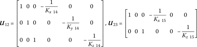
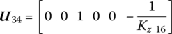
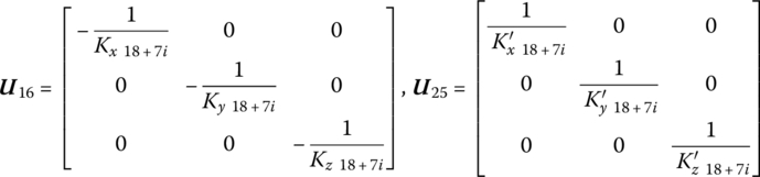
According to the principle of uniform numbering of body and joints in the MSTMM, the ground boundary is numbered 0, the six pairs of parallel springs and dampers connecting the wheels and the ground are numbered 1, 2, 3, 4, 5 and 6, the six wheels are numbered 7, 8, 9, 10, 11 and 12, the six pairs of parallel springs and dampers connecting the wheels and the vehicle are numbered 13, 14, 15, 16, 17 and 18, the vehicle, the revolving part and the elevating part are numbered 19, 21, 23, respectively, the action of the traversing mechanism and the connection between elements 19 and 21, the action of the elevating mechanism and the equilibrator and the parallel rotary spring, spring and damper between elements 21 and 23 are numbered 20 and 22, respectively, the two sets of parallel rotary springs, tension springs and dampers between the cradle and the ith launch tube are numbered ![]() and
and ![]() , respectively, the rear free boundary of the ith launch tube is numbered
, respectively, the rear free boundary of the ith launch tube is numbered ![]() , the ith launch tube trail is numbered
, the ith launch tube trail is numbered ![]() , the part between the front and rear bearing frames of the ith launch tube is numbered
, the part between the front and rear bearing frames of the ith launch tube is numbered ![]() , the front part of the front bearing frame of the ith launch tube is numbered
, the front part of the front bearing frame of the ith launch tube is numbered ![]() , and the front free boundary of the ith launch tube is numbered
, and the front free boundary of the ith launch tube is numbered ![]() . Therefore, the launch dynamics model of MLRS is a MRFS which is composed of 44 rigid bodies, 40 elastic bodies and 6 lumped masses, and connected with various springs, rotary springs and dampers under the action of ground support, jet flow and coupling between rocket and launch tube.
. Therefore, the launch dynamics model of MLRS is a MRFS which is composed of 44 rigid bodies, 40 elastic bodies and 6 lumped masses, and connected with various springs, rotary springs and dampers under the action of ground support, jet flow and coupling between rocket and launch tube.
In nature, the dynamics model of an MLRS is a nonlinear time‐varying system, whose nonlinear and time‐varying characteristics mainly come from three aspects:
- the nonlinear contact force between the rocket and tube caused by the rocket motion in the launch tube, the rocket‐tube clearance and the collision between the rocket and the tube
- the variance of contact stiffness between the ground and the wheels along with the variance of the total rocket number in the cradle
- the variance of the mass distribution of the MLRS caused by the variance of the total rocket number in the cradle and the position variance of the rocket motion in the launch tube during the launch process.
For these nonlinear factors the solutions are:
- the nonlinear contact forces caused by the rocket motion in the launch tube, the rocket‐tube clearance and the collision between the rocket and the guider are treated as “forcing forces”, that is, their influence on the dynamic response of the MLRS is considered, but their influence on the vibration characteristics of the MLRS is not considered
- the nonlinear contact stiffness between the ground and the wheels is expressed with subsection linear functions, that is, the value of contact stiffness is different along with the variance of the total rocket number in the cradle, which is decided by calculation and the static test result
- the variance of the total rocket number in the cradle will lead to a change in the vibration characteristics of the MLRS, and we can take this effect into account in this way: the variance of the total rocket number results in different mass and mass distribution of the elevating part, thus leading to different vibration characteristics.
Thus, the MLRS can be regarded as linear time‐invariant system during the firing round of every rocket. There are two reasons for the treatment methods: one is that there isn’t any strict computation method in theory for the vibration characteristics of a general linear time‐variant system at present; the other is that the result of the treatment method can meet the requirement of engineering precision because the mass of one rocket is only 1.5–4.0% of the elevating parts of the MLRS with 40 launch tubes, and the variance of natural frequency is very small between two near rocket rounds which have been validated by theory and test so it does not need to consider the variance of the system mode caused by the position variance of the rocket in the launch tube. The correctness of treating a nonlinear time‐variant system as a piecewise linear time‐invariant system has been proved by many test results and such treatment has high engineering precision.
12.3 State Vector, Transfer Equation and Transfer Matrix
12.3.1 State Vector
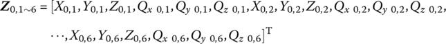
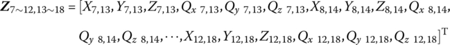
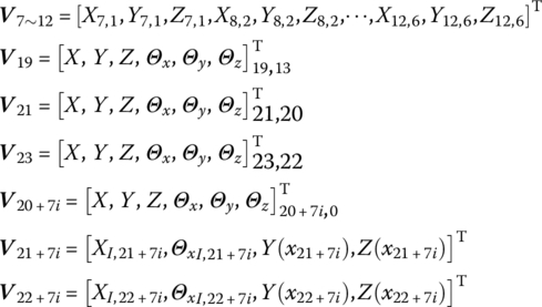
For the launch dynamics model of the MLRS shown in Figure 12.2, noting the sign convention, according to the MSTMM, the state vectors of the connection point of the MLRS are defined as follows:


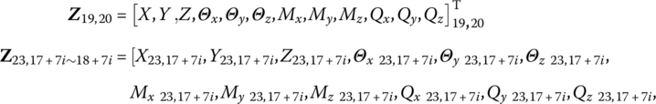
The form of ![]() ,
, ![]() ,
, ![]() ,
, ![]() ,
, ![]() ,
, ![]() ,
, ![]() , and
, and ![]() is similar to
is similar to ![]() , the subscripts denote the sequence number of bodies and joints at the connection point, and i is the sequence number of the launch tube.
, the subscripts denote the sequence number of bodies and joints at the connection point, and i is the sequence number of the launch tube.
12.3.2 Transfer Matrix and the Transfer Equation of a Component in the MLRS
12.3.2.1 From Ground to Wheels (axes)
According to the transfer equation of a spatial spring, the transfer equation from contact points between the wheels and the ground ![]() to the wheel (axle) points
to the wheel (axle) points ![]() can be obtained:
can be obtained:
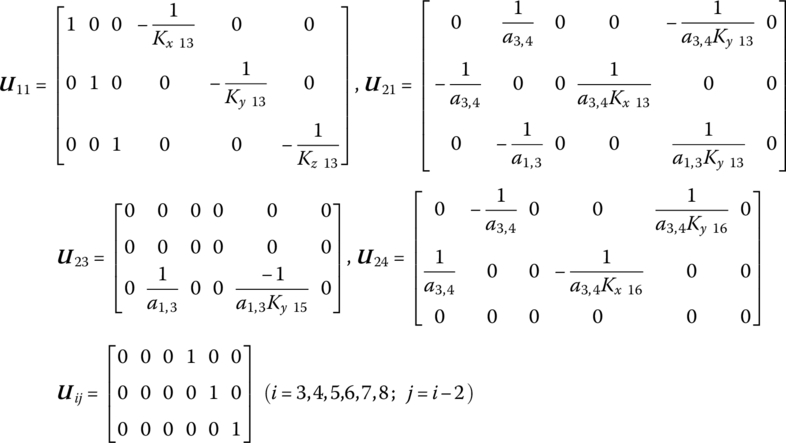
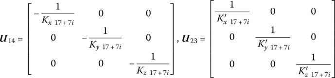
![]() is the transfer matrix from the ground to the wheels (axes):
is the transfer matrix from the ground to the wheels (axes):
where ![]() is the transfer matrix of the spatial spring.
is the transfer matrix of the spatial spring.
12.3.2.2 Wheels (axes)
According to the transfer equation of a lumped mass with spatial vibration, the transfer equation of the wheels (axes) from every axis point ![]() to point
to point ![]() can be obtained:
can be obtained:
![]() is the transfer matrix of the wheels (axes):
is the transfer matrix of the wheels (axes):
where ![]() is the transfer matrix of a lumped mass with spatial vibration.
is the transfer matrix of a lumped mass with spatial vibration.
12.3.2.3 From Wheels (axes) to Vehicle
According to the geometric and mechanic relation between the wheel (axes) points ![]() and the vehicle points
and the vehicle points ![]() , the transfer equations from the wheel (axes) points
, the transfer equations from the wheel (axes) points ![]() to the vehicle points
to the vehicle points ![]() can be obtained:
can be obtained:
where
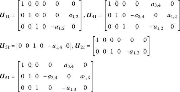
(a1,2, a2,2, a3,2), (a1,3, a2,3, a3,3), (a1,4, a2,4, a3,4), (a1,5, a2,5, a3,5), and (a1,6, a2,6, a3,6) are the coordinates of points (19, 14), (19, 15), (19, 16), (19, 17), and (19, 18) at the coordinate system whose origin is fixed on the first input end of body 19.
12.3.2.4 Vehicle
A vehicle is a rigid body with six inputs and one output. According to the transfer equation of a rigid body, the transfer equation from the vehicle points ![]() to (19, 20) can be obtained:
to (19, 20) can be obtained:
where ![]() is the transfer matrix of a rigid body (vehicle) with six input ends and one output end (see Equation (3.25)).
is the transfer matrix of a rigid body (vehicle) with six input ends and one output end (see Equation (3.25)).
12.3.2.5 Traversing Mechanism and Elevating Mechanism
The actions of traversing and elevating mechanisms are equivalent to the actions of rotary springs and springs. According to the transfer matrices of spatial springs and rotary springs, the transfer equations from the traversing mechanism point (19, 20) to point (21, 20) and from the elevating mechanism point (21, 22) to point (23, 22) can be obtained as, respectively,
where ![]() and
and ![]() are the corresponding transfer matrices of the elastic joints, respectively (see Equation (3.36)), and
are the corresponding transfer matrices of the elastic joints, respectively (see Equation (3.36)), and ![]() and
and ![]() are the corresponding coordinate transformation matrices with angles of azimuth α and departure angle θ, respectively.
are the corresponding coordinate transformation matrices with angles of azimuth α and departure angle θ, respectively.
12.3.2.6 Gyration Part
A gyration part is a rigid body with one input end and one output end. According to the transfer equation of a rigid body, the transfer equation of the gyration part can be obtained:
where ![]() is the transfer matrix of a rigid body (gyration part) with one input end and one output end (see Equation (3.19)).
is the transfer matrix of a rigid body (gyration part) with one input end and one output end (see Equation (3.19)).
12.3.2.7 Pitching Part
A pitching part is a rigid body with one input end and two output ends. According to the transfer equation of a rigid body, the transfer equation of the pitching part can be obtained:
where ![]() is the transfer matrix of a rigid body (pitching part) with one input end and two output ends.
is the transfer matrix of a rigid body (pitching part) with one input end and two output ends.
12.3.2.8 The ith Launch Tube Trail (to rear bearing)
Similar to the gyration part, the transfer equation of the ith launch tube rear end point ![]() to point
to point ![]() can be obtained:
can be obtained:
where ![]() is the transfer matrix of a rigid body (the ith launch tube trail) with one input end and one output end.
is the transfer matrix of a rigid body (the ith launch tube trail) with one input end and one output end.
12.3.2.9 Transfer Matrix of a Connection Point from the Pitching Part to the ith Launch Tube
The ith launch tube is connected to the pitching part through two points ![]() and
and ![]() , forming a loop between the pitching part and the launch tube. Using the geometric relation and the force equilibrium between point
, forming a loop between the pitching part and the launch tube. Using the geometric relation and the force equilibrium between point ![]() and point
and point ![]() , we obtain
, we obtain
Equation (12.22) can be written as
where
Similarly, using the geometric relation and the force equilibrium between point ![]() and point
and point ![]() , we obtain
, we obtain
where
The displacement (including angular displacement) relation between points ![]() and
and ![]() is
is
where

The displacement (including angular displacement) relation between points ![]() and
and ![]() is
is
namely
where
12.3.2.10 The ith Launch Tube
The ith launch tube in which the moving rocket is located is regarded as a transversely vibrating elastic beam, and its longitudinal and torsional deformation are neglected. The transfer equations from point ![]() to point
to point ![]() and from point
and from point ![]() to point
to point ![]() at the ith launch tube are, respectively,
at the ith launch tube are, respectively,
where ![]() and
and ![]() are the transfer matrices of transversely vibrating elastic beams without considering longitudinal and torsional deformation (see Equations (11.41) and (11.42)).
are the transfer matrices of transversely vibrating elastic beams without considering longitudinal and torsional deformation (see Equations (11.41) and (11.42)).
12.4 Overall Transfer Equation of the System
12.4.1 Transfer Equations from Ground (0, 1‐6) to Pitching Part 
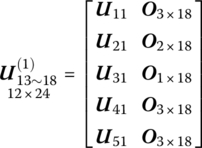
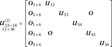
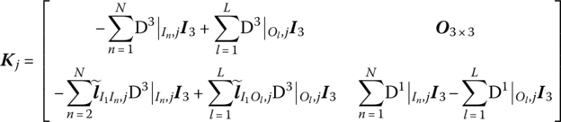
According to the transfer equations (12.7), (12.9), (12.11), (12.16), (12.17), (12.19), (12.18) and (12.20), the transfer equation from the ground to the pitching part can be obtained:
where
12.4.2 Transfer Equation from Ground  to Vehicle
According to the transfer equations (12.7), (12.9), (12.11) and (12.12), the transfer equation from point ![]() to point
to point ![]() can be obtained:
can be obtained:
where
12.4.3 Transfer Equation from Launch Tube Trail  to Launch Tube Muzzle
According to the transfer equations (12.21), (12.23), (12.33), (12.25) and (12.34), the transfer equation from point ![]() to point
to point ![]() can be obtained:
can be obtained:
where

12.4.4 Transfer Equation from Point  to Point
According to the transfer equations (12.21), (12.23), (12.33) and (12.29), we obtain
where
12.4.5 Transfer Equation from Point  to Point
According to the transfer equcations (12.21) and (12.27), we obtain
According to Equations (12.39) and (12.43), we obtain
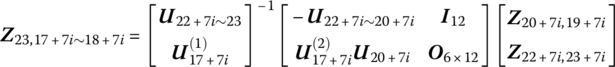
Let
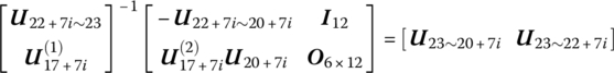
then
Substituting this into Equation (12.35) yields
Substituting this into Equation (12.41), it follows that
12.4.6 Overall Transfer Equation and Transfer Matrix of MLRS
According to Equations (12.37), (12.48) and (12.49), the overall transfer equation of MLRS can be obtained:
where
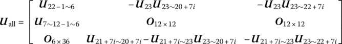
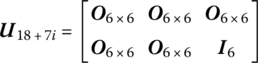
![]() is composed of state vectors at the boundary points of the system and
is composed of state vectors at the boundary points of the system and ![]() is the overall transfer matrix of the MLRS, a 30 × 60 matrix.
is the overall transfer matrix of the MLRS, a 30 × 60 matrix.
12.5 Vibration Characteristics of the System
The string firing of the MLRS means its vibration characteristics greatly influence the dynamic performance and firing precision, and the matching relation between firing frequency and vibration frequency has great influence on the dynamic performance, so it is necessary in dynamic design to compute the vibration characteristics of the MLRS and its change with a firing sequence at high speed. Because the total mass of the rocket is bigger than that of the launch tube, the mass of the rocket has a big influence on the vibration characteristics of the MLRS, which makes the vibration characteristics of the system different at every rocket round, so a large error will occur if the influence of the rocket mass on the vibration characteristics is not considered. In order to scientifically evaluate or ensure good dynamic performance and firing precision, the vibration characteristics of the MLRS must be expressed exactly and computed quickly, the quantitative relation between the total parameters of the MLRS and the vibration characteristics must be set up, and the vibration frequency distribution adjusted through altering the total parameters, which makes the vibration frequency match the firing frequency and improves firing precision. After the eigenvalues of the MLRS have been obtained, the dynamic response of the MLRS can be computed using the orthogonality of augmented eigenvectors.
Theory and test have proved that the firing sequence of the MLRS greatly influences the firing dispersion because different firing sequences can result in different vibration characteristics, different initial disturbance and different firing dispersion. The difficulty in solving the problem of quickly computing the vibration characteristics of the MLRS is the problems of too much computation work and computation error due to the “illness” when using the common mechanics method to compute the vibration characteristics of the MRFS. The “illness” in computing the vibration characteristics of the MRFS and the problem of quick computing are solved using the MSTMM. For example, for the MLRS with 40 launch tubes mentioned above, in order to ascertain the best firing precision by adjusting the firing sequence and the firing interval, only the optional schemes for firing sequence will reach 40! which is a surprisingly large number. It is first necessary to compute the vibration characteristics of every scheme when choosing the firing squence and the firing interval, so quickly computing the vibration characteristics of the MLRS is an important precondition to realize practical engineering dymanic design. In fact, it is these important and urgent engineering requirements that have led to the MSTMM being rapidly developed.
12.5.1 Characteristic Equation of the System
It is can be seen from Equation (12.51) that ![]() is composed of the state vectors at the boundary points of the system, including ground points
is composed of the state vectors at the boundary points of the system, including ground points ![]() , launch tube trail point
, launch tube trail point ![]() and launch tube muzzle
and launch tube muzzle ![]() . Half of the elements of the state vector at the boundary points are determined by the boundary condition. There are 36 elements in total in
. Half of the elements of the state vector at the boundary points are determined by the boundary condition. There are 36 elements in total in ![]() , including the displacement and force in three directions at six contact points between six wheels and the ground, where 18 elements respresenting displacement are zero. Getting rid of these zeros,
, including the displacement and force in three directions at six contact points between six wheels and the ground, where 18 elements respresenting displacement are zero. Getting rid of these zeros, ![]() can be written as
can be written as
The state vectors ![]() and
and ![]() of point
of point ![]() and point
and point ![]() include linear displacement, angular displacement, force and moment in three directions of corresponding points, and within the 12 elements involved in the state vector of each point, six of them (forces and displacements) are zeros. Getting rid of these zeros, we obtain
include linear displacement, angular displacement, force and moment in three directions of corresponding points, and within the 12 elements involved in the state vector of each point, six of them (forces and displacements) are zeros. Getting rid of these zeros, we obtain
Getting rid of these 30 zeros from ![]() , a new state vector can be obtained:
, a new state vector can be obtained:
Getting rid of columns 1, 2, 3, 7, 8, 9, 13, 14, 15, 19, 20, 21, 25, 26, 27, 31, 32, 33, 43, 44, 45, 46, 47, 48, 55, 56, 57, 58, 59, 60 in ![]() , a square matrix
, a square matrix ![]() with 30 orders can be obtained. Then Equation (12.50) is written as
with 30 orders can be obtained. Then Equation (12.50) is written as
or
It can be seen from the derivation process that both ![]() and
and ![]() are only relative to the total parameters of the system and the natural frequency
are only relative to the total parameters of the system and the natural frequency ![]() . When the total parameters of the system are determined, the determinant of matrix
. When the total parameters of the system are determined, the determinant of matrix ![]() corresponding to the natural frequency ωk is zero and Equation (12.58) must have a nontrivial solution, namely
corresponding to the natural frequency ωk is zero and Equation (12.58) must have a nontrivial solution, namely
Equation (12.59) is the eigenequation of the MLRS. Solving Equation (12.59), the eigenfrequency ![]() of the MLRS can be obtained. After the eigenfrequency
of the MLRS can be obtained. After the eigenfrequency ![]() of the MLRS is obtained, under the defined normalized condition (such as letting the maximal absolute value of the 30 elements of
of the MLRS is obtained, under the defined normalized condition (such as letting the maximal absolute value of the 30 elements of ![]() to be 1), solving Equation (12.58),
to be 1), solving Equation (12.58), ![]() and
and ![]() corresponding to ωk can be obtained, namely the state vectors
corresponding to ωk can be obtained, namely the state vectors ![]() ,
, ![]() and
and ![]() corresponding to ωk can be obtained. All state vectors (such as
corresponding to ωk can be obtained. All state vectors (such as ![]() ,
, ![]() , Z19,20, Z21,20, Z21,22,
, Z19,20, Z21,20, Z21,22, ![]() ,
, ![]() ,
, ![]() ,
, ![]() ,
, ![]() , and so on) at every connection joint and any point at the beam corresponding to ωk can be obtained through the transfer equation of each element.
, and so on) at every connection joint and any point at the beam corresponding to ωk can be obtained through the transfer equation of each element.
12.5.2 Vibration Characteristics of the System
Substituting the corresponding parameters into the characteristic equation and solving it, the natural frequency of the MLRS in any case can be obtained. The state vectors corresponding to natural frequency ![]() at any point of the MLRS can be obtained through the transfer equation of the system.
at any point of the MLRS can be obtained through the transfer equation of the system.
The quantitative relation between the vibration characteristics of the MLRS and the total parameters of the system is established. By changing the total parameters of the system, the vibration characteristics can be modified easily. The order of the transfer matrix and the eigenequation of the MLRS all are very low, which ensures the high‐speed computation of the vibration characteristics.
12.6 Dynamics Response of the System
In this section, the body dynamics equations of the MRFS for the MLRS are established, augmented eigenvectors which automatically satisfy orthogonality are constructed, and the way to exactly analyze the dynamics response of the multibody system for the MLRS is paved.
12.6.1 Body Dynamics Equations of the System
The body dynamics equation of single body element ![]() is
is
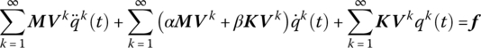
The body dynamics equation of every element is rearranged and assembled according to their sequence number, and so the body dynamics equation of the MLRS can be obtained:
where
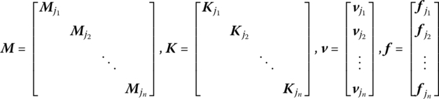
![]() is the column matrix of system displacement coordinates,
is the column matrix of system displacement coordinates, ![]() and
and ![]() are augmented operators,
are augmented operators, ![]() is the damping augmented operator,
is the damping augmented operator, ![]() is a column matrix of external force, and
is a column matrix of external force, and ![]() are the sequence numbers of the body element.
are the sequence numbers of the body element.
For proportional damping we have
where α and β are constant.
12.6.2 Orthogonality of Augmented Eigenvectors of the System
Let
where k is mode rank, q(t) is the generalized coordinate, and V is the augmented eigenvector of the MLRS.
The parameter matrices ![]() ,
, ![]() ,
, ![]() , and
, and ![]() of the body elements and the augmented eigenvector
of the body elements and the augmented eigenvector ![]() of the system are introduced in the following.
of the system are introduced in the following.
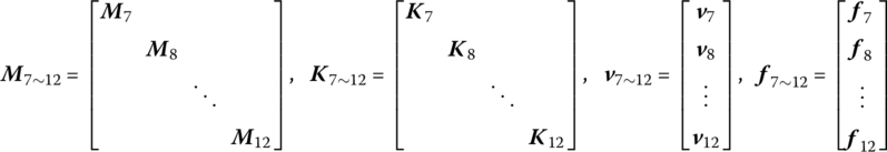
12.6.2.1 Six Wheels (Element  )
)
For six wheels, from Equation (5.7) we obtain
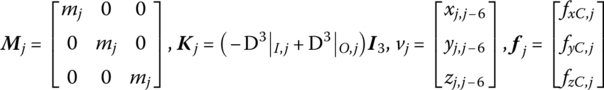
where mj is the mass of the wheel and [fxC,j, fyC,j, fzC,j]T is the column matrix of external force acting on the wheel.
For convenience, this is denoted as
12.6.2.2 Vehicle, Gyration Parts, Pitching Parts and Launch Tube Trail (Element 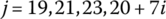 )
)
For the vehicle, gyration parts, pitching parts and launch tube trail, we obtain

where mj is the mass of rigid body j, C is the mass center, ![]() is the moment of inertia matrix about the first input end I1, [mxC,j, myC,j, mzC,j]T is the column matrix of external moment coordinates acting on the rigid body, [fxC,j, fyC,j, fzC,j]T is the column matrix of external force acting on the rigid body, In is the nth input point, and Ol is the lth output end.
is the moment of inertia matrix about the first input end I1, [mxC,j, myC,j, mzC,j]T is the column matrix of external moment coordinates acting on the rigid body, [fxC,j, fyC,j, fzC,j]T is the column matrix of external force acting on the rigid body, In is the nth input point, and Ol is the lth output end.
12.6.2.3 Launch Tube (Element 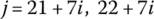 )
)
For the launch tube, if the lognitudinal and torsional deformations are neglected, we obtain
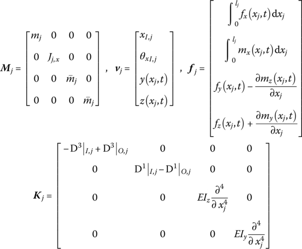
where xj are the coordinates of the point on elastic beam j, lj is the length of beam j, ![]() is the mass per unit length of beam j, EI is bending stiffness, mj is the total mass of beam j, mj=
is the mass per unit length of beam j, EI is bending stiffness, mj is the total mass of beam j, mj=![]() lj and Jj,x is the moment of inertia with respect to the axis of beam j.
lj and Jj,x is the moment of inertia with respect to the axis of beam j.
So we obtain

The augmented eigenvector ![]() of the MLRS is
of the MLRS is
where
From the orthogonality of the augmented eigenvectors of the multibody system established in this book, we obtain
where ![]() is the natural frequency of the system and Mp is the p th rank mode mass.
is the natural frequency of the system and Mp is the p th rank mode mass.
It is then possible to solve the dynamic responses of the MLRS once the following problems have been solved: calculating eigenvalues, constucting and verifying the orthogonality of the augmented eigenvectors, and establishing the launch dynamics equation of the MLRS. Some ways are offered here to calculate and analyze dynamics performance and the quantitative relation between dynamics performance and the total parameters of system, and the basis for decreasing rocket consumption in the MLRS test and improving the weapon performance is provided. As the multi‐uninterrupted firing weapon, the initial conditions of each firing and its vibration characteristics of corresponding system are different, and attention should be given to this when analyzing the dynamics response.
12.6.3 Dynamics Response of the System
Substituting Equations (12.64) and (12.63) into Equation (12.61), we obtain
Finding the inner products of ![]() and the terms on both sides of Equation (12.74), we obtain
and the terms on both sides of Equation (12.74), we obtain
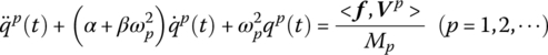
So ![]() can be obtained by substituting the column matrix of external force f and step‐by‐step integration of the above equation, using the Equation (12.64), gives the exact analysis of the dynamics response and high‐speed computation of the MRFS for the MLRS. This is an exact analysis because the difficult problem of orthogonality of eigenvectors of the MRFS for the MLRS is solved by the MSTMM, and it is a high‐speed computation because the problem of computation of eigenvalues and the dynamics response of the MRFS for the MLRS is also solved by the MSTMM, which ensures that the order of the involved matrix is low all the time, which cannot be achieved by other methods.
can be obtained by substituting the column matrix of external force f and step‐by‐step integration of the above equation, using the Equation (12.64), gives the exact analysis of the dynamics response and high‐speed computation of the MRFS for the MLRS. This is an exact analysis because the difficult problem of orthogonality of eigenvectors of the MRFS for the MLRS is solved by the MSTMM, and it is a high‐speed computation because the problem of computation of eigenvalues and the dynamics response of the MRFS for the MLRS is also solved by the MSTMM, which ensures that the order of the involved matrix is low all the time, which cannot be achieved by other methods.
12.6.4 Initial Value of Each Firing for the System
For the MLRS, the condition of the rocket launcher is changed with each rocket being fired, that is, when t is changed from ![]() to
to ![]() , the relative positions of point
, the relative positions of point ![]() , point
, point ![]() , point
, point ![]() , point
, point ![]() , and point
, and point ![]() are also changed. The mass, relative position of mass center, and inertial matrix of body 23 are changed, as are the eigenfrequency and eigenvector of the system. In this case, it is wrong to regard the numerical value of the response at time
are also changed. The mass, relative position of mass center, and inertial matrix of body 23 are changed, as are the eigenfrequency and eigenvector of the system. In this case, it is wrong to regard the numerical value of the response at time ![]() as that of time
as that of time ![]() directly. It is necessary to convert the response at time
directly. It is necessary to convert the response at time ![]() into the initial value of the dynamics response relative to the new balance position, and to deduce the system generalized coordinates in the new mode of the system from the initial value. Superscript i shows the squence number of the rocket fired, superscript + means after firing, while superscript – means before firing. Supposing the initial value of the system is known before firing the
into the initial value of the dynamics response relative to the new balance position, and to deduce the system generalized coordinates in the new mode of the system from the initial value. Superscript i shows the squence number of the rocket fired, superscript + means after firing, while superscript – means before firing. Supposing the initial value of the system is known before firing the ![]() th rocket, that is to say, the initial value at time
th rocket, that is to say, the initial value at time ![]() is known. How to determine the initial values of
is known. How to determine the initial values of ![]() and
and ![]() corresponding to the balance position when the system contains
corresponding to the balance position when the system contains ![]() rockets is as follows. The detailed calculation method can be seen in reference [1].
rockets is as follows. The detailed calculation method can be seen in reference [1].
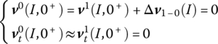
The weight of the rocket being fired is considered in the launch dynamics equations, and its action affecting the rocket launcher is embodied by contact force. The initial conditions of the dynamics response of the MLRS are displacement ![]() and velocity
and velocity ![]() when one rocket is fired, and the eigenvectoer, balance position and dynamics response relative to the balance position of the system excluding the fired rocket. Although the balance positions of the system in every firing are different, they are all static; the difference in the orientation angles of two neighboring balance positions caused by the weight of each rocket is small. So for two neighboring balance positions, the projections
when one rocket is fired, and the eigenvectoer, balance position and dynamics response relative to the balance position of the system excluding the fired rocket. Although the balance positions of the system in every firing are different, they are all static; the difference in the orientation angles of two neighboring balance positions caused by the weight of each rocket is small. So for two neighboring balance positions, the projections ![]() and
and ![]() of system velocity in the corresponding coordinate system can be regarded as being the same, where I is a point fixed on body 7,……, 12, 19, 21 or 23. In interval
of system velocity in the corresponding coordinate system can be regarded as being the same, where I is a point fixed on body 7,……, 12, 19, 21 or 23. In interval ![]() , the corresponding launch tube and rocket can be regarded as parts of body 23, so linear the displacement and angular displacement of every point at bodies
, the corresponding launch tube and rocket can be regarded as parts of body 23, so linear the displacement and angular displacement of every point at bodies ![]() ,
, ![]() and
and ![]() are determined by the rigid body motion of body 23.
are determined by the rigid body motion of body 23.
12.6.4.1 Initial Value of the First Rocket Being Fired
When the first rocket is fired, the other 39 rockets are contained in the system and the initial value relative to the balance position is

where ![]() is the displacement of point I at the moment of t relative to the balance position of the system when the launch tube contains
is the displacement of point I at the moment of t relative to the balance position of the system when the launch tube contains ![]() rockets,
rockets, ![]() represents the difference between the displacement relative to the balance position of the system when the launch tube contains
represents the difference between the displacement relative to the balance position of the system when the launch tube contains ![]() rockets and that when launch tube contains
rockets and that when launch tube contains ![]() rockets.
rockets.
When the first rocket is fired, the system initial value relative to the balance position of the system with a full load is
12.6.4.2 Initial Value of the Second Rocket Being Fired
When the second rocket is fired, the other 38 rockets are contained in the system. The mode shape of the system, the balance position and the dynamics response ![]() are all relative to the balance position of the system with 38 rockets, namely
are all relative to the balance position of the system with 38 rockets, namely
When the second rocket is fired, the system initial value relative to the balance position of the full‐load system is

12.6.4.3 Initial Value of the ith Rocket Being Fired
When the ith rocket is fired, there are ![]() rockets contained in the system. The mode shape of the system, the balance position and the response
rockets contained in the system. The mode shape of the system, the balance position and the response ![]() are all relative to the balance position of the system containing
are all relative to the balance position of the system containing ![]() rockets, namely
rockets, namely
When the ith rocket is fired, the initial value of the system relative to the balance position of the full‐load system is
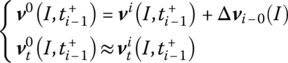
where
The initial values of each rocket are determined as shown above, including the values relative to the corresponding balance position and the balance position of the full‐load system. These values are used to calculate the dynamics response of the system at every period. Finally, these dynamics reponses of the system represented in their local equilibrium positions will be converted to the corresponding values represented in the initial (full‐load) equilibrium position.
12.6.5 Solving the Dynamics Response of the System
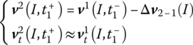
After the first rocket is fired, from the initial conditions we obtain

Solving Equations (12.74) and (12.75) and taking notice of Equation (12.83), qk(t), ![]() in interval
in interval ![]() , the dynamic response of the system, the rocket motion in the launch tube and the initial disturbance can be obtained.
, the dynamic response of the system, the rocket motion in the launch tube and the initial disturbance can be obtained.
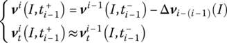
According to this calculation, ![]() ,
, ![]() , displacement
, displacement ![]() and velocity
and velocity ![]() at time
at time ![]() can also be obtained. Using Equation (12.78), displacement
can also be obtained. Using Equation (12.78), displacement ![]() and velocity
and velocity ![]() relative to the balance position of the system at time
relative to the balance position of the system at time ![]() (38 rockets are contained in the system) can be obtained. Similar to determining
(38 rockets are contained in the system) can be obtained. Similar to determining ![]() and
and ![]() ,
, ![]() and
and ![]() after the firing of the second rocket can be obtained. Using the augmented eigenvector Vk corresponding to interval
after the firing of the second rocket can be obtained. Using the augmented eigenvector Vk corresponding to interval ![]() , using Equations (12.73) and (12.75), qk(t),
, using Equations (12.73) and (12.75), qk(t), ![]() in interval
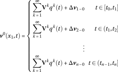
in interval ![]() , the dynamics response of the system, the parameters of rocket motion in the launch tube, and the initial disturbance can be obtained. Proceeding with this, the dynamics response of the system during the whole firing process can be obtained as follows:
, the dynamics response of the system, the parameters of rocket motion in the launch tube, and the initial disturbance can be obtained. Proceeding with this, the dynamics response of the system during the whole firing process can be obtained as follows:
12.7 Launch Dynamics Equation and Forces Acting on the System
12.7.1 Coordinate Systems
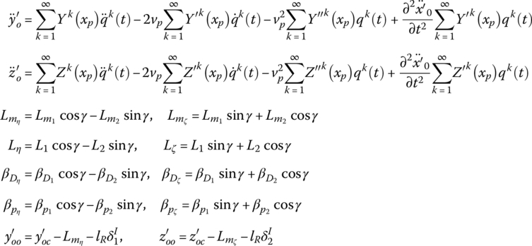
The o1xyz coordinate system (translational coordinate system): The origin o1 is attached to the geometric center of the rocket projectile at the initial position of the rocket, the x axis is directed toward the launch tube muzzle and along the tangent of the launch tube axis, the y axis is directed along the vertical plane and perpendicular to the x axis, and the z axis completes the triad, so the direction of every coordinate axis is then fixed. The system is mostly used to determine the basis of the orientation of the rocket, as shown in Figure 12.3.
Figure 12.3 Translational coordinate system and inertial coordinate system.
The ooxoyozo coordinate system (rocket launcher coordinate system): The origin oo is the crosspoint of the cross‐section of the rocket at the mass center and launch tube axis. The xo axis is directed toward the launch tube muzzle and along the tangent of the launch tube, the yo axis is directed along the vertical plane and perpendicular to the xo axis, and the zo axis completes the triad. The system is used to determine the basis of the orientation of the rocket relative to the launch tube.
The o1ξηζ coordinate system (rocket projectile coordinate system): The origin o1 is attached to the geometric center of rocket projectile, the ξ axis is directed toward the head of the rocket and along the geometric longitudinal axis of the rocket, the η axis is directed along the vertical plane and perpendicular to the ξ axis, and the ζ axis completes the triad. As shown in Figure 12.4, the system is used to determine the orientation of the rocket axis.
Figure 12.4 Rocket axis coordinate system and translational coordinate system.
The o1x2y2z2 coordinate system (velocity coordinate system): The origin o1 is attached to the geometric center of the rocket projectile, the x2 axis is directed toward the velocity of the geometric center of the rocket, the y2 axis is directed along the vertical plane and perpendicular to the x2 axis, and the z2 axis completes the triad. As shown in Figure 12.5, the system is used to determine the translation of the rocket.
Figure 12.5 Rocket axis coordinate system and velocity coordinate system.
12.7.2 Forces Analysis of the Launching Process
Forces on the MLRS include weight, the mechanic interactive forces among the components and between the MLRS launcher and the ground, the projectile‐launcher action force, the thrust of the engine, the impact force of the jet flow and so on. Mechanic interactive forces among components and between the MLRS launcher and the ground may be equivalent to the corresponding spring and damping forces of elastic joints with damping, which are all internal forces of the system. In solving the launch dynamics of the MLRS using the MSTMM, the supporting forces of the ground are included in the system dynamic model as internal forces, and these internal forces are all considered in the state vector and need not be expressed with intricate external forces. These are also features of solving the launch dynamics of the MLRS by the MSTMM.
The static balance position of the system is regarded as the basis of system displacement, where the rockets fired and being fired are not included in the system. In this way, the function of system weight (including all components and the rocket not fired) in dynamics equations is offset by that of the static deformation of system components, so in the chosen coordinate system the action related to the weight of the system and the static deformation need not be considered, which greatly simplifies the forces analyzed and the dynamics solved for the MLRS. The large impact force on the rocket launcher [265] is made by the rocket exhaust, which causes vibration of the rocket launcher. The initial disturbance of the subsequently fired rocket is affected, and the firing dispersion of the MLRS is also affected. The forces between the rocket and the launch tube are a pair of acting forces and counterforces. The kinetic equation of the rocket launcher and the vibration equation of the rocket launcher couple together, via the interaction force between bourrelet and launch tube, as well as the interaction force between the guide button and the guide trough. These forces include the normal collision force and the tangential friction force between the bourrelet and the launch tube, and between the guide button and the guide trough. That the weight of the fired rocket affects the rocket launcher is demonstrated by the contact force between the rocket and the launcher. The thrust of the engine and the impingement force of the rocket exhaust on the firing equipment can be calculated theoretically or measured by testing.
The forces acting on the rocket in the launch tube include weight, the thrust of the engine, air resistance, as well as the force between the launch tube and the guide button, and the contact force between the bourrelet and the launch tube. The expressions are given in reference [1].
12.7.3 The Launch Dynamics Equation of the Rocket
As launch dynamics is very complex, the launch dynamics of a multibody system such as an MLRS with high temperature, high pressure, short time and violent change cannot be solved using the usual kinds of research methods. In the research field and the expansive literature of launch dynamics at home and abroad, the model of launch dynamics has had to be simplified again and again, so the differences between the model and the reality are so great that the resulting level of error is large. In launch dynamics research an assumption is always made by the researcher that the rear bourrelet center moves along the bore axis as this simplifies the research problem. In 1984, the general differential equation of motion of a projectile in a bore was developed by Marting, an American expert in weapon dynamics [266]. To overcome the shortcomings of the Marting’s equation, a uniform launch dynamics equation of a rocket suitable for all kinds of motion has been established by the authors. Not only are the factors considered more general and closer to reality than those of Marting’s model, but also the form of the differential equation of motion is more concise than that of Marting’s equation. In the model of launch dynamics, the rocket weight, thrust, thrust tmalalignment angle, linear thrust malalignment, rocket‐tube clearance, contact force between bourrelet and launch tube, mass eccentricity, and dynamic unbalance are all considered. The translational and rotational equations are established in the rocket launcher coordinate system ooxoyozo and the rocket axis system o1ξηζ, respectively [1].
The general dynamics equations of an asymmetric rocket in the launch tube are
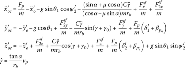
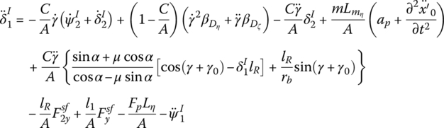

where
![]() ,
, ![]() and
and ![]() are the longitudinal, vertical and sidewise accelerations, respectively, of the mass center of the rocket projectile in the rocket launcher coordinate system ooxoyozo,
are the longitudinal, vertical and sidewise accelerations, respectively, of the mass center of the rocket projectile in the rocket launcher coordinate system ooxoyozo, ![]() ,
, ![]() and
and ![]() are the projections in the rocket launcher coordinate system ooxoyozo of acceleration of the mass center of the rocket launch tube with respect to the ground coordinate system, Fp is thrust, μ is the frictional coefficient between the guide button and the launch tube, m is the mass of the rocket, θ1 is the departure angle of the rocket launcher, γ is the roll angle of the rocket, γ0 is the initial orientation angle of the guide slot, g is the acceleration due to gravity, ap is the axial acceleration at the origin point oo of the rocket launcher coordinate system ooxoyozo for launching the tube,
are the projections in the rocket launcher coordinate system ooxoyozo of acceleration of the mass center of the rocket launch tube with respect to the ground coordinate system, Fp is thrust, μ is the frictional coefficient between the guide button and the launch tube, m is the mass of the rocket, θ1 is the departure angle of the rocket launcher, γ is the roll angle of the rocket, γ0 is the initial orientation angle of the guide slot, g is the acceleration due to gravity, ap is the axial acceleration at the origin point oo of the rocket launcher coordinate system ooxoyozo for launching the tube, ![]() and
and ![]() are the vertical and sidewise components of the contact force
are the vertical and sidewise components of the contact force ![]() between the rear bourrelet and the launch tube, respectively, and
between the rear bourrelet and the launch tube, respectively, and ![]() and
and ![]() are the vertical and sidewise components of the contact force
are the vertical and sidewise components of the contact force ![]() between the front bourrelet and the launch tube, respectively.
between the front bourrelet and the launch tube, respectively. ![]() and
and ![]() are the vertical and sidewise components of the bracket angle between the projectile spin axis and the tangent of the launch tube axis,
are the vertical and sidewise components of the bracket angle between the projectile spin axis and the tangent of the launch tube axis, ![]() and
and ![]() are the projections of thrust malalignment angle βp in axes η and ζ of the rocket axis coordinate system o1ξηζ, respectively, α is the twist angle of the guide flute, rb is the neutral circular radius of the guide button,
are the projections of thrust malalignment angle βp in axes η and ζ of the rocket axis coordinate system o1ξηζ, respectively, α is the twist angle of the guide flute, rb is the neutral circular radius of the guide button, ![]() and
and ![]() are the vertical and sideways components of the bracket angle between the tangent of the launch tube axes and the aiming line, respectively, A is the transverse moment of inertia of the rocket, C is the polar moment of inertia,
are the vertical and sideways components of the bracket angle between the tangent of the launch tube axes and the aiming line, respectively, A is the transverse moment of inertia of the rocket, C is the polar moment of inertia, ![]() and
and ![]() are the projections of dynamic unbalance angle
are the projections of dynamic unbalance angle ![]() in axes η and ζ of the rocket axis coordinate system o1ξηζ, respectively,
in axes η and ζ of the rocket axis coordinate system o1ξηζ, respectively, ![]() and
and ![]() are the projections of mass eccentricity
are the projections of mass eccentricity ![]() in axes η and ζ of the rocket axis coordinate system o1ξηζ, respectively, Lη and Lζ are the projections of thrust malalignment
in axes η and ζ of the rocket axis coordinate system o1ξηζ, respectively, Lη and Lζ are the projections of thrust malalignment ![]() in axes η and ζ of the rocket axis coordinate system o1ξηζ, respectively, lR is the distance between the mass center of the rocket and the rear bourrelet, and l1 is the distance between the mass center of the rocket and the front bourrelet.
in axes η and ζ of the rocket axis coordinate system o1ξηζ, respectively, lR is the distance between the mass center of the rocket and the rear bourrelet, and l1 is the distance between the mass center of the rocket and the front bourrelet.
12.8 Dynamics Simulation of the System and its Test Verifying
On the basis of the launch dynamics of the MLRS based on the MSTMM, the 6‐DOF rigid‐body ballistics model [267, 268] is adopted, the influence of the aerodynamic force of the rocket, mass, mass eccentricity, dynamic unbalance, propellant mass, thrust, linear thrust malalignment, thrust malalignment angle, gusts of wind, and other random factors relevant to flight process are considered synthetically, and the flight dynamics model and the dynamics equation of the MLRS are established, although they are omitted here and can be seen in reference [1]. Combining with the launch and flight dynamics of the MLRS, the dynamic performance of the weapon system from ignition in the rocket engine to the rocket impacting the ground in the MLRS can be studied. The firing and flying process of the MLRS is influenced by many random factors, including the random change in the parameters of the rocket, launcher and propellant, the randomness of the application environment (weather condition, ground condition etc.) and the handling process (personnel technical diathesis, handling error ect.), and so on. There are two main ways of handling firing and flying dynamics problems for the MLRS: the deterministic model, where the random factors of the firing and flying process are not considered, and the random model, where the random factors of the firing and flying process are considered. The deterministic model handles system problems in isolation, so it is difficult to obtain satisfying analysis results for the firing and flying process for the MLRS. By starting from the view of a system of rocket, launcher, propellant and circumstance, and studying the firing and flying process by applying the random model, the essence of the launch process can be revealed, and the regular pattern of the launch dynamics can be found. The Monte Carlo method is an efficient way to solve the random model.
Random simulation is a numerical method of finding the approximate solution of mathematical, physical, engineering and other problems by simulation and statistical tests. It studies the dynamic process and characteristics of the simulated system by numerical experiment. The core of launch dynamics simulation is the random‐firing and flying‐dynamics equation, which is based on the MSTMM established by the author. The detailed processes are as follows. Based on the statistical characteristics (such as the mean value and mean‐square deviation) of a random variable (such as rocket mass, mass eccentricity, dynamics unbalance, propellant mass, thrust, linear thrust malalignment, thrust malalignment angle, firing interval, rocket‐tube clearance, bending property, gust wind, and so on), generate the corresponding random variable sequence by using the random simulation principle. Then, regard the launch dynamics equations as deterministic equations and carry out several times of certain computation. For each of the certain computations, the random variables are assigned with a set of certain values chosen from the random variable sequence. The statistical characteristics of corresponding parameters in the random firing and flying dynamics process can be obtained by computing these results. According to the eigenequations, the augmented eigenvector and its orthogonality conditions, the launch dynamics and ballistics equations, the random launch dynamics simulation system of the MLRS based on the MSTMM is established and can be used to study the influence of random or nonrandom factors on firing dispersion. The simulation results are validated by vibration characteristics, dynamic response, and the ballistic and firing dispersion of the MLRS, which also validate the theory and simulation system of the MLRS based on the MSTMM.
12.8.1 Composition, Flow and Functions of the Simulation System
The launch dynamics simulation system of the MLRS based on the MSTMM is as follows:
- General control module: This module is used to mobilize all function modules, simulate the launch dynamics, carry out the statistical analysis and output the results.
- Random number module: This module produces the random number for other the function modules according to the statistical characteristics of the random parameter, which are prescribed by a specified distribution.
- Weapon vibration characteristics module: This module is used to simulate the eigenfrequency, eigenvector, damping ratio and so on.
- Interior ballistics module: This module is used to simulate the thrust and interior ballistics with the random number obtained in (2) as one part of the basic parameter.
- Impingement force of the rocket exhaust module: This module is used to simulate the impingement force of the rocket exhaust.
- Weapon dynamic characteristics of the firing process module: This module is used to simulate projectile and barrel motion, projectile–barrel interaction, and the initial disturbance of the rocket according to the data obtained in (2), (3), (4) and (5).
- Exterior ballistics module: This module is used to simulate the ballistics data of the rocket projectile and hitting point scattering according to the data obtained in (2), (4) and (6).
- Statistical analysis module: This module is used to deal with the simulation results statistically.
- Correlation analysis module: This module is used to analyze correlation among all kinds of factors, the dynamic performance of the MLRS and the firing accuracy according to the data obtained in (2), (6) and (7), to offer the primary influence factors of dynamic performance of the MLRS and the firing accuracy, and to provide the basis for the general parameter dynamic design of the MLRS.
- Result output module: This module is used to output simulation results in the form of character, curve and figure etc.
The simulation flow of the launch dynamics of the MLRS based on the MSTMM is shown in Figure 12.6.

Figure 12.6 Simulation flow of the launch dynamics of an MLRS based on the MSTMM.
The functions of the launch dynamics simulation system based on the MSTMM are:
- Simulation of the vibration characteristics of the MLRS and its variance caused by the variance of the total rocket number in the launcher.
- Simulation of the dynamic response of the MLRS (including displacement, velocity, acceleration, angular displacement, angular velocity, angular acceleration etc.).
- Simulation of the initial disturbance of the rocket (including initial swing angle, initial swing velocity, muzzle rotation angle, rotation angular velocity, displacement, velocity, and other motion parameters).
- Simulation of exterior ballistics and firing precision of the MLRS (including exterior ballistics data, ballistics parameters of burning phase end, flight time, points of fall, firing accuracy, firing dispersion, etc.).
12.8.2 Simulation Results of the Dynamics Response of the System
The firing sequence and the loading position of a MLRS with 40 launch tubes are shown in Figure 12.7. The loading position of every rocket is denoted with a dual (n1, n2), where n1 shows the row number with 1, 2, 3 and 4 from up to down, while n2 shows column number with 1, 2… 10 from left to right. In the figure, each circle represents a launch tube, the nearside number inside the circle represents the firing sequence of a 40‐rocket salvo, and the dextral number inside the circle represents the loading position of the rockets. For example, the loading position of the 26th rocket in the firing sequence is represented by (4, 6).
Figure 12.7 Firing sequence and loading position of an MLRS with 40 launch tubes.
Using the launch dynamics simulation system of the MLRS based on the MSTMM, the launch dynamic simulation results of a MLRS with 40 launch tubes and rockets in the process of firing are obtained as follows.
12.8.2.1 Simulation Results of the Launch Dynamics of a MLRS with Single Firing
The numerical simulation of an MLRS with 40 launch tubes single firing was carried out. Some of the simulation results of the launch tube vibration during single tube firing are shown in Figures 12.8–12.17. The time histories of the motion and the impact forces of the rocket are illustrated in Figures 12.18–12.27.
Figure 12.8 Muzzle displacement in the x direction.

Figure 12.17 Muzzle angular velocity in the y direction.
Figure 12.18 Lognitudinal displacement of the rocket.
Figure 12.27 Impact force of the aft bourrelet.
12.8.2.2 Simulation Results of the Launch Dynamics of a MLRS with a 40‐rocket Salvo
The numerical simulation for an MLRS with a 40‐rocket salvo was carried out. Some of the numerical simulation results are shown in Figures 12.28–12.43.
Figure 12.28 Muzzle displacement in the x direction.


Figure 12.42 Muzzle angular acceleration in the x direction.
Figure 12.43 Muzzle angular acceleration in the y direction.
12.8.3 Simulation Result of the Initial Disturbance of the Rocket
The initial disturbance of an MLRS with 40 launch tubes is simulated by the launch dynamics simulation system of the MLRS based on the MSTMM. Some of the numerical simulation results are shown in Table 12.1.
Table 12.1 Simulation results of initial disturbance of rocket
| Swing angle | Swing angular velocity | Yaw angle | ||||
| φa/rad | φ2/rad | ψ1/rad | ψ2/rad | |||
| Mean value | 0.866 | −2.03 × 10⁻⁵ | −0.102 | −5.07 × 10⁻³ | −4.19 × 10⁻³ | −9.45 × 10⁻⁴ |
| Mean square | 4.96 × 10⁻⁵ | 5.61 × 10⁻⁵ | 3.03 × 10⁻³ | 2.40 × 10⁻³ | 6.27 × 10⁻⁵ | 6.04 × 10⁻⁵ |
12.8.4 Simulation and Test Validation of the Vibration Characteristics of the System
The simulation results and the mode test results of the first 14 eigenfrequencies of an MLRS with 40 launch tubes under the condition of full‐load and non‐load are shown in Tables 12.2 and 12.3, respectively. The comparison indicates that they have good agreement, and the simulation results are validated by a modal test.
Table 12.2 Comparision of simulation and modal test results of eigenfrequencies under the condition of full‐load
| Mode, k | ωk/(rad/s) | Relative error/% | Mode, k | ωk/(rad/s) | Relative error/% | ||
| Compute | Test | Compute | Test | ||||
| 1 | 8.61 | 8.67 | –0.69 | 8 | 52.77 | 50.27 | 4.97 |
| 2 | 10.40 | 10.99 | –5.37 | 9 | 57.43 | 56.23 | 2.13 |
| 3 | 19.33 | 18.98 | 1.84 | 10 | 60.39 | 64.34 | –6.14 |
| 4 | 26.67 | 26.51 | 0.60 | 11 | 66.05 | 67.61 | –2.31 |
| 5 | 28.93 | 29.59 | –2.23 | 12 | 80.06 | 79.73 | 0.41 |
| 6 | 31.99 | 32.86 | –2.65 | 13 | 97.86 | 97.89 | –0.03 |
| 7 | 36.82 | – | – | 14 | 105.62 | 105.81 | –0.18 |
Table 12.3 Comparison of simulation and modal test results of eigenfrequencies under the condition of non‐load
| Mode, k | ωk/(rad/s) | Relative error/% | Mode, k | ωk/(rad/s) | Relative error/% | ||
| Compute | Test | Compute | Test | ||||
| 1 | 10.72 | 10.93 | –1.92 | 8 | 41.37 | 37.51 | 10.29 |
| 2 | 13.03 | 12.32 | 5.76 | 9 | 50.30 | 50.20 | 0.20 |
| 3 | 17.88 | – | – | 10 | 58.74 | 55.54 | 5.76 |
| 4 | 23.56 | 24.44 | –3.60 | 11 | 75.68 | 71.94 | 5.20 |
| 5 | 26.27 | 25.01 | 5.04 | 12 | 90.98 | 92.05 | –1.16 |
| 6 | 27.17 | 29.97 | –9.34 | 13 | 98.13 | 97.45 | 0.70 |
| 7 | 31.75 | 34.49 | –7.94 | 14 | 108.75 | 110.65 | –1.72 |
12.8.5 Simulation and Test Validation of the Vibration of the System
The simulation results and test results for the vehicle response of an MLRS with a salvo of 40 launch tubes are shown in Figure 12.44 (departure angle is 50°, azimuth angle is 45°) and the simulation results and test results of the vehicle response when firing 16 rounds with the B scheme are shown in Figure 12.45. It is obvious that the simulation and test results have good agreement. The simulation results are validated by the tests.
Figure 12.44 Simulation and test results of the vertical displacement of a vehicle when salvo firing.
Figure 12.45 Simulation and test results of the vertical displacement of a vehicle with B scheme.
12.8.6 Simulation and Test Verifying of Firing Dispersion
The simulation and test results for firing dispersion at a certain range of an MLRS with 40 launch tubes are shown in Table 12.4 and show good agreement. The simulation results are also validated by the tests.
Table 12.4 Simulation and test results of firing dispersion
| EX/m | EZ/m | |
| Simulation | 73.7 | 222.0 |
| Test | 73.3 | 208.9 |
12.9 Low Rocket Consumption Technique for the System Test
The question of whether or not the weapon performance fulfils the tactical‐technical criteria must be answered by a shooting test when the weapon is approved to be used. In test for firing dispersion, generally three groups of firing test are carried out under each of the conditions of high, low and normal temperature, and the number of firing rounds of each group for firing of the MLRS is “the number in one salvo”, that is to say, it is necessary to fire nine groups for a full‐load salvo test. Taking the Russian БM‐21 type MLRS with 40 launch tubes as an example, one salvo needs 40 rockets, thus at least 360 rockets will be consumed to assess its firing dispersion at maximum range. For another Russian MLRS with 12 launch tubes, one salvo needs 12 rockets, thus 108 rockets will be consumed to assess its firing dispersion at maximum range. As a result a lot of ammunition and a vast test budget are required to check the dispersion at maximum range.
In this section, for a whole system, including rocket, gun, propellant and environment, using the theory of MLRS launch dynamics based on the MSTMM, a totally new programmed firing dispersion test technology that substitutes a non‐full charge loading test for a full charge loading test is introduced, which greatly reduces the rocket consumption in the MLRS test. Many tests show that the rocket consumption for the firing dispersion of the MLRS of several National High‐Tech Projects is decreased by 50–86% compared to the usual methods, and is the lowest level in the world.
12.9.1 Principle of Decreasing Rocket Consumption in MLRS Tests
12.9.1.1 Launch Dynamic Principle of Decreasing Rocket Consumption in MLRS Tests
The grouping test method is usually used in testing the firing dispersion of MLRSs. Its advantages are as follows:
- By grouping the rockets in the test, the firing time for the same number of rockets is relative short for each group, which reduces the influence of gusts of wind, temperature and other factors on firing dispersion, so the firing dispersion of the weapon system is more accurately and objectively reflected.
- Using a limited number of firing rounds, the error in the dispersion test caused by operation, settling guns and other factors can be eliminated or greatly reduced by taking an average value after each grouped test.
The National Military Standard regulates that the dispersion test for an MLRS should use the grouping test method [269].
Decreasing rocket consumption in the MLRS test means that, using this new theory and technology, the rocket consumption in an MLRS test is much less than with the current test scheme when evaluating and checking MLRSs under the precondition of ensuring checking accuracy. The method of decreasing the rounds used in each group should be adopted to decrease rocket consumption in MLRS testing under the precondition that the quality of the test is guaranteed.
The theory of launch dynamic and firing tests shows that there are three main factors that influence the firing dispersion of MLRSs: (i) the initial disturbance of the rocket, (ii) factors of the rocket itself (such as mass, mass eccentricity, dynamic unbalance, propellant mass, thrust malalignment and so on) and (iii) the meteorological conditions (such as wind). The influences of the vibration chatacteristics of the MLRS, the performance of the MLRS, the loading scheme of the rockets and the firing sequence on firing dispersion are embodied in the initial disturbance of the rocket. For single‐round firing, only factors of the rocket itself and the firing dispersion influence the factors of rockets and gusts of wind, thus seven rounds in each group are capable of giving sufficiently precise results according to the engineering precision demand. For the same MLRS, the firing dispersion of a full‐load salvo or seven rounds of string firing in one go is different from that of single‐round firing. However, when rockets have stable performance, the influence of factors of the rocket itself including weight, diameter, mass eccentricity, dynamic unbalance, thrust malalignment, etc.) on the firing dispersion in every group for these two conditions (a full‐load salvo and seven rounds of string firing in one go) is not large. Therefore, for the same MLRS, the main reason for a large difference in firing dispersion between a full‐load salvo and nonfull‐load string firing is the difference in initial disturbance for these two situations. This viewpoint has been validated by firing tests for MLRSs over many years.
Applying the theory and technology of launch dynamics based on the MSTMM, and optimizing the total parameters of the MLRS, the vibration characteristics of the MLRS, the dynamic response, the trajectory and the dispersion can be realized according to the scheduled distribution law under different firing schemes. The nonfull‐charge loading test scheme can then be found whose firing dispersion is the same as that of the full‐charge loading test. A firing dispersion test in which the nonfull‐charge loading test is substituted for a full‐charge loading test can be done. The rocket number (seven, for example) of nonfull‐charge loading must assure the demand for assessing the influence of factors of rocket itself on firing dispersion. So, the replacement of the dispersion test of full‐charge loading by nonfull‐charge loading should be carried out based on the fact that there is no distinct difference between the two estimating values of firing dispersion of the MLRS under the two cases. This is the basic principle of decreasing the rocket consumption in the MLRS test via the theory and technology of launch dynamics.
12.9.1.2 Statistics Principle of Decreasing Rocket Consumption in the MLRS Test
The impact coordinates are random variables and are usually considered to have a normal distribution. The distance coordinate of the impact point is given by x and the transverse coordinate by z. Both these show normal distribution and are independent from each other, so the situation can be explained by discussing only distance x. The probability pE(n) is called the confidence level of the estimated value ![]() located in interval
located in interval ![]() . For different DOFs
. For different DOFs ![]() (where n is the number of test rounds), the probability is pE(n) and the value
(where n is the number of test rounds), the probability is pE(n) and the value ![]() is found from the computation where
is found from the computation where ![]() is the confidence level of estimated value
is the confidence level of estimated value ![]() located in interval
located in interval ![]() when testing infinite rounds and
when testing infinite rounds and ![]() denotes the confidence level of replacing the estimated value
denotes the confidence level of replacing the estimated value ![]() of infinite rounds by estimated value
of infinite rounds by estimated value ![]() of n rounds. The confidence levels of the estimation of the mean and its variation tendency along with the number of test rounds are shown in Table 12.5 and Figure 12.46.
of n rounds. The confidence levels of the estimation of the mean and its variation tendency along with the number of test rounds are shown in Table 12.5 and Figure 12.46.
Table 12.5 Confidence level of estimation for mean along with test rounds (ta = 0.6745)
| n | 3 | 4 | 5 | 6 | 7 | 8 | 9 | 10 | 40 | |
| pE(n) | 0.429 | 0.450 | 0.461 | 0.469 | 0.474 | 0.477 | 0.480 | 0.482 | 0.496 | 0.50 |
 |
0.858 | 0.900 | 0.922 | 0.938 | 0.948 | 0.954 | 0.960 | 0.964 | 0.992 | 1 |
Figure 12.46 Histogram of change in  along with test rounds.
It can be seen from Table 12.5 and Figure 12.46 that when the number of test rounds bigger than seven, the confidence level increases very slowly and at the same time the confidence level reaches then exceeds 94.8% of that of the infinite rounds test. Therefore, for the same batch of ammunition with steady performance and single‐round firing with a launch tube, only seven rounds are needed to describe the influence of random factors of the rocket itself on the mean value of the coordinates of the points of fall.
When estimating firing dispersion, we usually suppose that it is a random variable with normal distribution. E is the system firing dispersion and its estimated value is Ê, where ![]() and
and ![]() . The probabilities (confidence level) of the estimated value
. The probabilities (confidence level) of the estimated value ![]() of the standard deviation located in interval
of the standard deviation located in interval ![]() are shown in Table 12.6 and Figure 12.47 for
are shown in Table 12.6 and Figure 12.47 for ![]() . This is also the probability (confidence level) of the estimated value Ê of the dispersion located in interval
. This is also the probability (confidence level) of the estimated value Ê of the dispersion located in interval ![]() . The probability (confidence level) of the estimated value Ê located in interval
. The probability (confidence level) of the estimated value Ê located in interval ![]() is therefore 91.7% for seven test rounds with a launch tube. Table 12.6 and Figure 12.47 show that when the number of test rounds is more than seven, confidence level increases slowly as number of test rounds increases.
is therefore 91.7% for seven test rounds with a launch tube. Table 12.6 and Figure 12.47 show that when the number of test rounds is more than seven, confidence level increases slowly as number of test rounds increases.
Table 12.6 Confidence level of estimation for mean square deviation along with test rounds
| n | 3 | 4 | 5 | 6 | 7 | 8 | 9 | 10 | 40 | |
| Confidence level | 0.682 | 0.779 | 0.842 | 0.886 | 0.917 | 0.938 | 0.954 | 0.966 | 0.999 | 1 |
Figure 12.47 Confidence level of estimation for mean square deviation along with test rounds.
Taking both of these factors into account, firing seven rounds is the routine method for the firing dispersion test of a weapon with a single launch tube for the same batch of ammunition with steady performance, the basis being that the corresponding confidence level of the estimated value of the firing dispersion can reach 91.7%. For an MLRS with 40 launch tubes, if the number of test rounds is bigger than seven in one group the confidence level of the estimated value of the firing dispersion should reach 91.7%. If the influence of factors such as coupling between the rocket and the gun on firing dispersion is considered, it is necessary to optimize the loading position, firing sequence and firing interval when searching the test scheme, substituting the nonfull‐charge loading test for the full‐charge loading test.
12.9.2 Programming Technology of Substituting Nonfull Loading for Full Loading
A difficult engineering problem that urgently needs to be solved is how to optimize and design a system that includes random and discrete variables at the same time because the existing theories and methods of optimization design cannot do this. Because of the low efficiency of optimization design for discrete variables and the sample effect of mathematical statistics which results in huge computational work, it is difficult to determine the optimal solution for the global area. Compared with the case of continuous variables, the optimization design of discrete variables has many different characteristics, such as the discontinuity of the variable, the discontinuity of the feasible area space (feasible area becomes feasible assemblage), the undifferentiability of the function, the nonapplicability of the Kuhn–Tucker condition and so on. These features make the optimization design for discrete variables different to that for continuous variables. Not only is the selection method for the chosen design variable different, but the judgement condition of optimization is also different. To address this problem, a totally new method for optimization design, random integer programming, has been developed by the authors. In this method, the continuity, discrete, randomicity and hypothesis tests of design variables are considered, with the aim of first ascertaining the necessary solution space and then solving the optimal solution. Thus, the difficult problem, namely that optimization design for discrete variables based on statistics cannot be used in large engineering due to its low computation efficiency, is overcome. The engineering optimization problem of decreasing rocket consumption in the firing dispersion test of an MLRS is also solved using this method. This method has been verified and further details can be found in reference [1].
The general approach to decreasing rocket consumption in the firing dispersion test of an MLRS is to take the MLRS system as research background, synthetically apply the new theory and technology of launch dynamics based on the MSTMM, adjust the loading position, firing sequence and firing interval of the nonfull‐loading scheme, and search the nonfull‐loading scheme whose firing dispersion is same as that of the original 40‐rocket full‐loading scheme. In this way rocket consumption in the MLRS test can be freatly decreased as long as the test quality is assured.
The detailed procedure to decrease rocket consumption in the firing dispersion test of the MLRS is to apply the newest study results for the launch dynamics based on the MSTMM, along launch scheme → initial disturbance of rocket → dispersion of the MLRS, taking the theory of launch dynamics of the MLRS as the foundation, the launch dynamics simulation system as the core, the random integer programming [1] as a tool, using the same firing dispersions for two systems as the constraint condition, taking the minimum rocket consumption as the target, by mean of adjusting loading position, firing sequence and firing interval, through plenty of computation and optimization, getting a new test scheme, and inspecting whether the estimated values of firing dispersion for the two schemes are distinctly different with statistical methods. Thus, the new test scheme substituting full loading with non‐full loading for dispersion test of MLRS can be found. The programmed technology for decreasing rocket consumption in the MLRS test by substituting full loading with nonfull loading is shown in Figure 12.48. The steps involved are as follows:
- Select the applicable launch dynamics model of the MLRS from the library of models and determine the statistical property (such as mean and standard deviation) of the correlated parameters according to measured parameters.
- Using the launch dynamic simulation system of the MLRS based on the MSTMM, carry out simulations for the firing dispersion of the MLRS.
- Optimize the test scheme, substituting full loading with nonfull loading for dispersion of the MLRS using random integer programming.
Figure 12.48 Programming technology with low rocket consumption in an MLRS test.
12.9.3 Optimization of a Nonfull‐load Firing Scheme and Test Verifying
When determining a nonfull‐loading MLRS system A1 to simulate the firing dispersion of a full‐loading salvo, random integer programming is used to optimize the firing dispersion test scheme of the MLRS. The factors that influence the dispersion of the MLRS are divided into two types, one is decided by the inherent mechanics characteristics of the rocket‐launcher system and the other is decided by various random factors. The main influence of the inherent mechanics characteristics of a rocket‐launcher system on firing dispersion is the change in the initial disturbance of the rocket due to the difference in rocket‐launcher vibration produced by the mass and stiffness of the rocket launcher, firing sequence, interval of the rocket, rocket exhaust and so on.
The main influence of various random factors is the change in rocket ballistics caused by the randomness of parameters such as rocket‐tube clearance, dynamic unbalance, mass eccentricity, thrust malalignment and firing interval. For the same batch of rockets, with steady performance and the same rocket launcher, the statistical properties of various random parameters are steady, their influence on firing dispersion is rather slight, but the variance of the inherent mechanics characteristics of the MLRS (including loading position, firing sequence, and so on) is main factor that influences the variance of the firing dispersion. The influence of these factors on firing dispersion must be fully considered when determining a test scheme. The firing dispersion EA of the MLRS is a multivariable function that has the following form:
where ![]() is a constant structure parameter of the system which influences firing dispersion,
is a constant structure parameter of the system which influences firing dispersion, ![]() is the rocket loading position vector (
is the rocket loading position vector (![]() ), xi is an integer variable equal to 0 or 1, and
), xi is an integer variable equal to 0 or 1, and ![]() is the mean of firing interval t.
is the mean of firing interval t.
Let ![]() ,
, ![]() ,
, ![]() , and
, and ![]() . The random part
. The random part ![]() of the firing interval
of the firing interval ![]() is considered in
is considered in ![]() , where
, where ![]() is a random vector that influences the firing dispersion (such as mass of rocket, thrust, thrust malalignment, dynamic unbalance, mass eccentricity, propellant mass, the random part of firing interval, or weather condition). Because the influence of random vector
is a random vector that influences the firing dispersion (such as mass of rocket, thrust, thrust malalignment, dynamic unbalance, mass eccentricity, propellant mass, the random part of firing interval, or weather condition). Because the influence of random vector ![]() and constant structure parameter
and constant structure parameter ![]() on the firing dispersion EA of full‐load salvo system A0 and nonfull‐load system A1 is steady,
on the firing dispersion EA of full‐load salvo system A0 and nonfull‐load system A1 is steady, ![]() and
and ![]() are the main factors causing a difference in the firing dispersion between the two systems.
are the main factors causing a difference in the firing dispersion between the two systems. ![]() and
and ![]() are the main design variables when determining the nonfull‐loading system, and the influence of various random factors on system firing dispersion and the discontinuity of
are the main design variables when determining the nonfull‐loading system, and the influence of various random factors on system firing dispersion and the discontinuity of ![]() must be considered at the same time. The following discrete variable mathematical programming problem based on statistics is constructed:
must be considered at the same time. The following discrete variable mathematical programming problem based on statistics is constructed:
where y is the target function, xi is the loading position function of the rocket for the MLRS with 40 launch tubes, ![]() , where xi is an integer equal to 0 or 1, xi = 0 means there is no loading rocket in the ith position of the launch tube and xi = 1 means a rocket is loaded in the ith launch tube.
, where xi is an integer equal to 0 or 1, xi = 0 means there is no loading rocket in the ith position of the launch tube and xi = 1 means a rocket is loaded in the ith launch tube. ![]() is a hypothesis test of the firing dispersion of the full‐load salvo system A0 and the target system A1.
is a hypothesis test of the firing dispersion of the full‐load salvo system A0 and the target system A1.
On the foundation of the launch dynamics of the MLRS based on the MSTMM, using the method of random integer programming [1], the nonfull‐load system A1 is obtained with an estimated value of firing dispersion that is not distinctly different from that of the full‐load salvo system A0, so the firing test scheme substituting full‐load salvo with nonfull‐load is obtained:
- number of rounds in each group: 7
- firing interval: 0.5 ± 0.05 s
- loading position and firing sequence: 1 (2,6), 2 (3,6), 3 (4,5), 4 (1,7), 5 (2,4), 6 (2,7), 7 (3,4).
In Figure 12.49 each circle represents a launch tube, the number on the left of each circle represents the original firing sequence in a 40‐round salvo, and the number on the right of each circle represents the new firing sequence in the seven‐round string firing scheme. The serial numbers of the launch tube corresponding to the seven‐round string firing scheme are 6, 22, 28, 10, 16, 14, and 32.
Figure 12.49 Test scheme of nonfull loading with seven rounds.
According to the static measure results for the rocket (including rocket weight, mass eccentricity, eccentricity position, bourrelet diameter and so on), using the established simulation system, the firing dispersions of the seven‐round string firing scheme and the original 40‐round salvo are numerically simulated. The variance trends for firing dispersion along with the number of firing groups for the seven‐round string firing scheme and the original 40‐round salvo scheme are shown in Figure 12.50, and the critical values of the F test is shown at the same time. It can be seen from the predicted results that the variation tendencies of the firing dispersions of the two schemes share the same pattern as the number of the test groups increases, and the firing dispersions always meet the requirement of the F test, which shows that the two schemes have the same firing dispersion. In order to verify the correctness of the seven‐round string firing scheme, special dispersion contrast tests for both the seven‐round string firing scheme and the 40‐round salvo scheme are completed. The test results prove that the seven‐round string firing scheme is correct and the test technology for the firing dispersion of the MLRS substituting full‐charge loading with nonfull‐charge loading is effective. The simulation and test results for the firing dispersion of the seven‐round string firing scheme and the 40‐round salvo are shown in Table 12.7 and are in good agreement. The F test shows that there are no distinct differences between the test results for the seven‐round string firing scheme and the 40‐round salvo when ![]() , so the system firing dispersions of the two launch schemes are the same, which validates the seven‐round optimization test scheme.
, so the system firing dispersions of the two launch schemes are the same, which validates the seven‐round optimization test scheme.
Figure 12.50 The variance trends for firing dispersion along with the number of firing groups for the seven‐round string firing scheme and the original 40‐round salvo scheme, as well as the critical values of the F test.
Table 12.7 Simulation and test results of firing dispersion of seven rounds of firing and 40‐round salvo
| Launch scheme | EX/m | EZ/m | |
| Simulation | 40‐round salvo | 74.1 | 207.1 |
| Seven rounds of string firing | 74.8 | 206.8 | |
| Test | 40‐round salvo | 73.3 | 208.9 |
| Seven rounds of string firing | 80.2 | 198.0 |
The following conclusions can be drawn from the test results:
- The simulation results are validated by the test, and the launch dynamics theory of the MLRS based on the MSTMM is also validated.
- The test results for the firing dispersion of the seven‐round firing scheme and the 40‐round salvo are same, so the seven‐round optimization test scheme is validated, which shows that the technology for decreasing rocket consumption in the MLRS test is right and that the rocket consumption in the firing dispersion test of the MLRS is decreased by 82.5% compared to the common method.
The difficult problem of decreasing rocket consumption in the MLRS test was solved by the test technology. Under the precondition of ensuring test quality, the test budget greatly decreases when the firing dispersion test of the MLRS of the full‐loading salvo is substituted with the nonfull‐loading scheme, and such a substitution has good operability and can be easily applied in engineering practice.
12.10 High Launch Precision Technique for the System
Precise striking is one of the main goals for modern weapons, and the firing dispersion of weapons is given great attention by all countries. In this section, the MLRS firing technology established by authors of high precision and little initial disturbance using the theory of multibody system launch dynamics based on the MSTMM is introduced. Real firing tests have shown that the firing precision and firing dispersion of several MLRSs in the National High‐Tech Project are greatly improved, the corresponding research period is short, and the cost of the research is low.
12.10.1 Technique for Improving the Firing Dispersion of the System
A lot of research for improving the firing dispersion of the MLRS has carried out by rocket experts all over the world. The concept of passive control [270–272] for improving firing dispersion was first put forward by John E. Cochran. The basic idea is that the ballistic difference caused by the initial disturbance of the rocket could be counteracted by the ballistic difference caused by thrust malalignment, dynamics unbalance and mass eccentricity by a thorough study of the amplitude frequency and phase frequency response function of the launch equipment. The main purpose of passive control is to improve the firing dispersion, mainly by reducing the angular velocity dispersion of the deflection angle at the end of the power period. No outside energy source is needed, the control is realized only by using the feedback of rocket launch system itself and the control sources are rocket’s own random factors. Although passive control looks tempting in theory, the model is very simple, which is very important in reality because it lacks a way of establishing the quantitative relation between the total parameters of the MLRS and its dynamic performance. This means it is difficult to reach the goal of reducing initial disturbance through adjusting the total parameters of the MLRS, and so far there has been no practical application of this result. It is, however, an important way of using simple control to improve the firing accuracy of the MLRS, for example a rocket with simple control has been used in the Russian PC30 CMEPЧ MLRS and the US M270 MLRS, and is being developed in Italy, Britain and other countries to improve the firing accuracy of the MLRS. The cost of a rocket with simple control is several times higher than that of an ordinary rocket. The search continues around the world for a new method of improving the firing accuracy of the MLRS.
The firing technology of an MLRS with high precision has been established by the authors using the theory and method of MSTMM launch dynamics. The main features of this technology are as follows:
- Through optimizing the parameters of the rocket‐launcher system (such as firing sequence and firing interval) the initial disturbance can be reduced.
- Using the concept of equivalent initial disturbance, through the design of the parameters of the rocket‐launcher system, the initial disturbance of the rocket counteracts the equivalent initial disturbance caused by its own deficiency (mass eccentricity, dynamics unbalance, thrust malalignment and other factors). In addition, the ballistic difference caused by the initial disturbance of the rocket is counteracted by the ballistic difference caused by its own deficiency.
- The integration soft/hard module of launch dynamics is installed on a rocket launcher to control the initial disturbance of the rocket by controlling the motion of the launch tube of the MLRS. This greatly reduces the cost of improving the firing precision of noncontrol MLRSs compared to using simple control. This method and its application in improving the firing dispersion of an MLRS by reducing the initial disturbance due to optimizing the firing sequence and firing interval are discussed in this section.
The MLRS is a kind of string‐firing weapon, and its firing sequence and firing interval have a very big influence on its dynamic performance. It has been shown that different firing sequences and different total system parameters will lead to different vibration characteristics and different initial conditions for each rocket fired, resulting in different initial disturbance of the rocket. The matching relation between the firing frequency and the natural frequency also largely influences dynamic performance, and a reasonable firing interval is very important to ensure and improve firing dispersion. Therefore, the goal of improving the firing dispersion of the MLRS through reasonable adjustment of the firing sequence and firing interval can be achieved.
12.10.2 Random Combinatorial Optimization for Firing Dispersion
How can we optimize the firing sequence and firing interval to ensure the highest firing dispersion of the MLRS? For an MLRS with n launch tubes, there are n ! kinds of firing sequences. To obtain the optimum solution for the whole area, all kinds of firing sequences must be scanned one by one. If a group of calculations is taken as one scan, the total computation time is about 1.2 quadrillion years using a PIV‐3.2G computer, which is not feasible. In addition, the theory and algorithm of global optimization is not as advanced as that of local optimization, so the analysis condition similar to the condition “gradient is zero and the second derivative matrix is orthogonality” of the local minima point has not yet been achieved, that is to say, it there is not an affirmative method of judging whether or not a local minima point is a global minima point. Even the filling function method, a kind of global optimization algorithm proposed in recent years, can only solve an optimization problem whose target function is analytical expression of continuous variables and whose constructed filling function is an analytical function about target function and optimization variables, which is useless for an optimization problem about discrete variables. Because it is difficult to find an optimal solution of global area, many approximation algorithms have been constructed, including the greed method, the local scanning method and the incomplete enumeration method. These methods behave better in seeking preferable solutions. Based on these methods, focused on the essence of the problem, the arithmetic of random combinatorial optimization is constructed, in which a random combination is adopted in each optimization and every combination is forbidden to repeat the former. Thus, the local optimal solution can be searched and the firing dispersion of the original system is improved to meet engineering requirements.
In order to find the local optimal solution, a constraint condition for the firing sequence is first decided according to the research results of MLRS launch dynamics. The firing sequency (from far to near) is symmetrical about the center of the launcher, and the rocket nearest to the center of the launcher is fired at last. Next, a random firing sequence is produced, which must satisfy the constraint conditions, and the firing dispersion is simulated corresponding to the firing sequence combination and estimated using the maximum entropy method. Lastly, the hypothesis test is applied to judge whether or not the firing dispersion is higher than that of original firing sequence. After many random combinatorial optimizations, the firing sequence corresponding to a high firing dispersion can be obtained. In fact, the key to improve the firing dispersion via the optimization of the firing sequence is that the firing dispersion of the MLRS corresponding to different firing sequences can be simulated exactly, and the optimization of the firing sequence is merely a combinatorial optimization problem of mathematics. The flowchart for random combinatorial optimization is shown in Figure 12.51.
Figure 12.51 Flow of random combinatorial optimization.
12.10.3 High Firing Dispersion Scheme and its Test Verification
Taking the launch dynamics simulation system of the MLRS to be a platform based on the MSTMM, the influences of various factors on firing dispersion, such as rocket, launcher, propellant and environment, are all taken into consideration, and the firing sequence and firing interval of the optimization firing scheme are obtained using random combinatorial optimization. The simulation results for the corresponding relation between firing interval and firing dispersion for an MLRS are shown in Figure 12.52, from which it can be seen that a reasonable firing interval for the weapon system is 1.0 s.

Figure 12.52 Relations between firing interval and firing dispersion.
Many test results have indicated that firing dispersion is improved more than four times by the optimization scheme relative to the original firing sequence and firing interval.