
13
Dynamics of Self‐propelled Launch Systems
13.1 Introduction
The launch process affects the characteristics of weapon systems in many ways, especially the firing precision. The influence of artillery characteristics on the scattering of projectiles can only be evaluated by the initial disturbances of the projectiles as a result of the launching process. The interaction between projectile and artillery during the launch process must be fully considered and the initial disturbance must be accurately computed when analyzing and computing the weapon system. How to solve the difficult problem of self‐propelled artillery is a practical example of the important engineering applications of the linear transfer matrix method for multibody system (MSTMM) introduced in this chapter [106–111]. Self‐propelled artillery weapon systems, which are widely equipped all over the world, are chosen as our study object in this chapter. Using MSTMM, self‐propelled artillery is regarded as a multi‐rigid‐flexible‐body system (MRFS). The natural vibration characteristics of the system are computed first, then the body dynamic equations of the system are established and the augmented eigenvector and its orthogonality are constructed, and finally the dynamic response and initial disturbance of the projectile are solved. The simulation system for the launch dynamics of self‐propelled artillery is also formed, which provides an important tool for the dynamic design to improve the firing precision and other aspects of weapon performance.
13.2 Dynamics Model of the System and its Topology
The launch process of a projectile refers to the whole process from the moment that the primer is fired to the end of the period during which the projectile is affected by the gas that ejects from the gun muzzle. The movements of the artillery and the projectile are very complex during the launch process because of the complex structure of the self‐propelled artillery and the extreme environment, such as high temperature, high pressure and high speed. The complexity of the launch process is shown in four interactions: between the projectile and the artillery, between the transverse motion and the longitudinal motion, between the rigid body and the flexible body, and between the space coordinates and the time coordinates for the motion parameters. The launch dynamics model of self‐propelled artillery is a very complex mechanics multibody system connected in certain modes that contain many rigid bodies and flexible bodies with large motion.
13.2.1 Dynamic Model of a Self‐propelled Launch System
The M109A6 155‐mm type self‐propelled artillery (USA) is shown in Figure 13.1. The main components of self‐propelled artillery are the muzzle device, barrel (including an evacuator), gun breech, recoil and counterrecoil mechanism, cradle, pitching mechanism, equilibrator, turret, traversing mechanism, chassis (artillery bogie), torsion bar, balance elbow, shock absorber, track chain and road wheel. According to the motion state of each component, the firepower system of self‐propelled artillery can be divided into recoil, lifting, turning, sprung, walking and so on. The recoil part contains the muzzle device, barrel, gun breech, recoil and counterrecoil mechanism. The lifting part contains the total recoil part, cradle and the elements moving with cradle, which include the elevating mechanism, equilibrator and so on. The turning part contains the total lifting part, turret and the elements moving with turret, which include the traversing mechanism and so on. The walking part, which contains track chain and road wheels, is used to support the weight of self‐propelled artillery and drive the self‐propelled artillery to run smoothly. The sprung part is used to connect the chassis to the walking part, which contains the torsion bar, balance elbow and shock absorber.
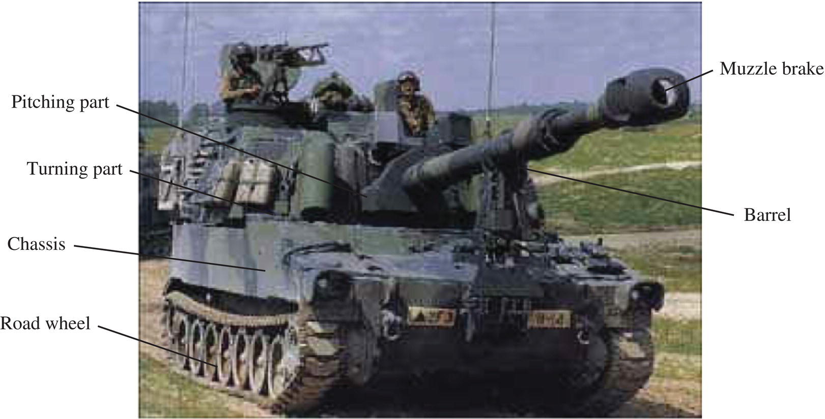
Figure 13.1 M109A6 type 155 mm self‐propelled artillery (USA).
The components of self‐propelled artillery are arranged from bottom to top in sequence, that is, road wheels, chassis without road wheels (simplified called hull, including carriage and sprung part), traversing mechanism, turning parts which do not contain the lifting part (the revolving part), elevating mechanism and equilibrator, lifting part without recoil part (the pitching part), gun breech, barrel and muzzle brake. Self‐propelled artillery can thus be divided into 12 road wheels, barrel (partitioned into six segments), hull, revolving parts, pitching part, gun breech and muzzle brake. The launch dynamic model of self‐propelled artillery is shown in Figure 13.2. The road wheels are regarded as lumped masses. The hull, revolving part, pitching part, gun breech and muzzle brake are regarded as rigid bodies. The barrel is divided into six segments and each is regarded as a beam with equal sectional area. Therefore, the whole structure contains 12 lumped masses, 6 elastic beams and 5 rigid bodies. The ground that supports the self‐propelled artillery is regarded as an infinity rigid body. The elastic and damping effects of each road wheel, the interaction between the ground and each road wheel, and the connection between each road wheel and the hull are modeled as springs and dampers in three directions. The effect of the traversing mechanism associated with the elastic and damping effects of the hull, the effect of the elevating mechanism and equilibrator associated with the elastic and damping effects between the revolving and pitching parts, and the interaction between the barrel and the pitching part are modeled as springs and rotary springs accompanying dampers which can represent relative linear motion and relative angle motion in three directions at the same time. The connections between barrel and gun breech, the connection between the barrel and the muzzle brake, and the connection between each segment of the barrel are regarded as fixed connections. The masses of the traversing mechanism, the elevating mechanism and the equilibrator are divided into the pitching part, the revolving part and the hull, respectively. The launch dynamics model of self‐propelled artillery is therefore an MRFS composed of 23 bodies and 28 joints.
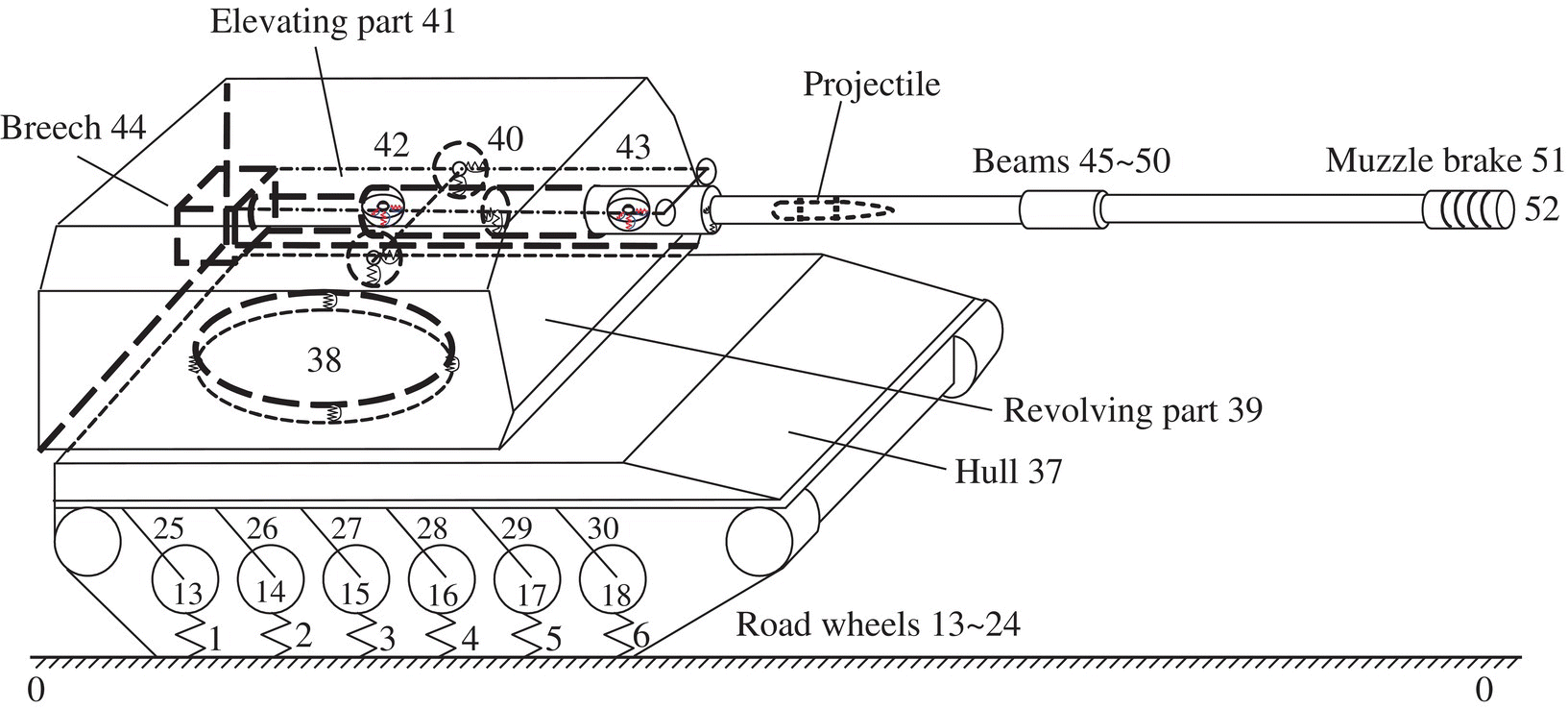
Figure 13.2 Launch dynamic model of self‐propelled artillery.
Each element is numbered, and there are ![]() elements in all, so
elements in all, so ![]() . The system has three boundaries: ground, gun breech and muzzle. The ground is regarded as the first input end, the gun breech is the second input end and the muzzle is the output end, therefore the muzzle boundary is numbered
. The system has three boundaries: ground, gun breech and muzzle. The ground is regarded as the first input end, the gun breech is the second input end and the muzzle is the output end, therefore the muzzle boundary is numbered ![]() . Both the ground boundary and the gun breech boundary are numbered 0. The other elements are numbered in sequence, as shown in Figure 13.2. All the interaction forces and moments between barrel and pitching part, pitching part and revolving part, revolving part and hull, hull and road wheels, road wheels and the ground during the launch process are regarded as internal forces. To deal with vibration characteristics easily, the recoil resistance between the barrel and the pitching part produced by the recoil and counterrecoil mechanism is decomposed into two parts, the external force and the internal force, and the internal force is proportional to the relative displacement between the barrel and the pitching part. All the forces acting on the barrel by the projectile and propellant gas, and acting on the muzzle brake by the propellant gas are regarded as external forces of self‐propelled artillery.
. Both the ground boundary and the gun breech boundary are numbered 0. The other elements are numbered in sequence, as shown in Figure 13.2. All the interaction forces and moments between barrel and pitching part, pitching part and revolving part, revolving part and hull, hull and road wheels, road wheels and the ground during the launch process are regarded as internal forces. To deal with vibration characteristics easily, the recoil resistance between the barrel and the pitching part produced by the recoil and counterrecoil mechanism is decomposed into two parts, the external force and the internal force, and the internal force is proportional to the relative displacement between the barrel and the pitching part. All the forces acting on the barrel by the projectile and propellant gas, and acting on the muzzle brake by the propellant gas are regarded as external forces of self‐propelled artillery.
13.2.2 Launch Dynamic Model of a Projectile
Because of the complexity of the problem, the launch dynamic model of a projectile moving in a gun tube has to be simplified. As a result of the derivation from the actual models, the mathematical modal of a projectile moving in a gun tube reported in the literature on launch dynamics often results in large computation errors. In the past, the hypothesis “the center of the rotating band moves along the axes of the gun tube” was proposed to simplify the problem. To address the deficiency of past research, this hypothesis has been abandoned by the authors. The main body of a projectile is regarded as a rigid body and the elastic effect of the projectile is equal to the elastic effect of the rotating band and bourrelet. Almost all factors are considered, including the dynamic unbalance, mass eccentricity, gravity, pressure of propellant gas, resistance acted on the head of projectile by air, rotating band/bore contact force, bourrelet/bore contact force and corresponding moment.
13.2.3 Dynamic Model of Interior Ballistics Two‐phase Flow
The configuration of ammunition for self‐propelled artillery is shown in Figure 13.3. It is a separated cartridge with a metal cartridge case. Its charge includes granular propellant and a metal central ignition tube. When the cartridge primer is fired, the gas jet of the primer ejects into the ignition tube. Then the ignition powder in the central ignition tube is ignited systematically, and the burning gas produced makes the pressure and temperature of the gas in the ignition tube rise continually. When the pressure is high enough to break the ignition holes on the ignition tube, the ignition gas flows into the propellant bed, which is ignited, and the increase in propellant burning gas makes the pressure in the chamber rise sharply. When the pressure at the end of the projectile is high enough the projectile begins to move. Subsequently, the propellant grains and burning gas flow into the barrel. During the ignition process and burning propagation in the chamber, gas flow is stopped due to the existence of solid propellant grain, causing a gradient of speed and pressure. The asymmetric distribution of propellant grains occurs due to the mutual action between the gas phase and the solid phase. The propellant bed moves to the end of the projectile due to the pressure difference in the chamber, then stacks and collides. At the same time, various waves are reflected at the end of the projectile, resulting in an inverted pressure gradient that forces the propellant bed to move back toward the breech. There is mutual movement and action between the solid phase and the gas phase before the propellant is finished burning, which forms a complex two‐phase flow movement in the gun tube.
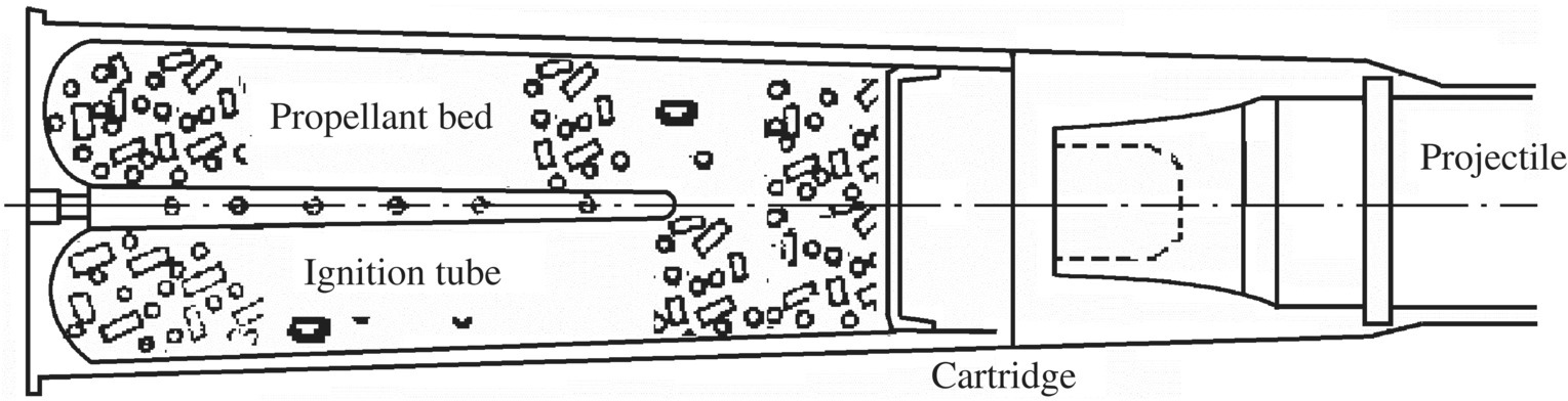
Figure 13.3 Configuration of propellant charge for large caliber self‐propelled artillery.
To deal with this problem, one‐dimensional grids and the one‐dimensional two‐phase flow model are adopted in the main charge and in the central ignition tube, respectively. Between these two areas mass, momentum and energy are exchanged. Interphase drag, interphase heat transfer, the ignition process of the solid phase, the stress between solid propellant grains, the engraving of the projectile, the resistance of the projectile moving in the gun tube and other factors are considered. The basic hypotheses are:
- The main charge is regarded as a continuous medium.
- In the ignition tube only gas flows, solid grains do not flow and only gas can spurt out from the ignition holes on the ignition tube.
- Both flows in the gun tube and the ignition tube are one‐dimensional, and the state parameters in the same section are constant.
- There is only a gas phase and a solid phase in the gun tube, and the solid phase cannot be compressed.
- Combustion of propellant obeys the geometric burning law and the exponential law of burning rate.
- Burning gas obeys the Nobel–Abel gas state equation.
- The viscosity of the gas is omitted, as is the heat lost from the wall of the gun tube.
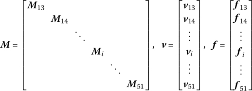
13.3 State Vector, Transfer Equation and Transfer Matrix
13.3.1 State Vector
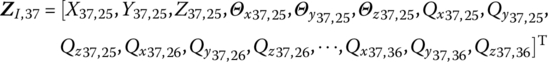
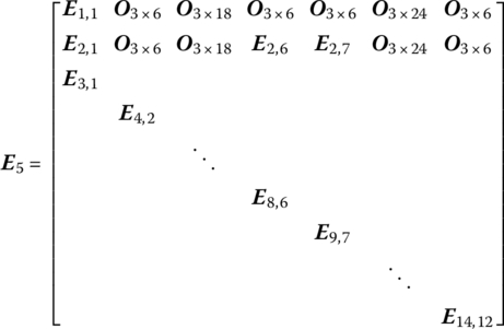
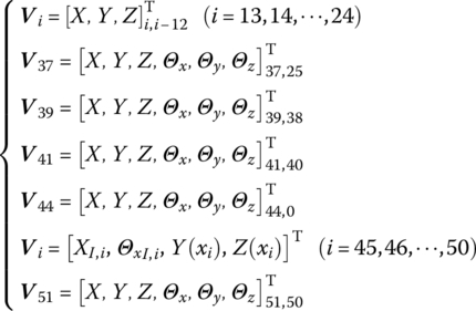
According to the launch dynamic model of self‐propelled artillery and the sequence number of each element, there are 49 connection points (![]() ,
, ![]() ,
, ![]() , P37,38, P39,38, P39,40, P41,40, P41,42, P41,43, P44,45, P45,46, P46,47, P47,48, P48,49, P49,50 and P51,50) and 14 boundary points (
, P37,38, P39,38, P39,40, P41,40, P41,42, P41,43, P44,45, P45,46, P46,47, P47,48, P48,49, P49,50 and P51,50) and 14 boundary points (![]() , P44,0, P51,52), therefore 63 state vectors are defined as follows
, P44,0, P51,52), therefore 63 state vectors are defined as follows
The form of ![]() ,
, ![]() and
and ![]() is similar to Equation (13.1), and the form of
is similar to Equation (13.1), and the form of ![]() ,
, ![]() ,
, ![]() ,
, ![]() ,
, ![]() ,
, ![]() ,
, ![]() ,
, ![]() ,
, ![]() ,
, ![]() ,
, ![]() ,
, ![]() ,
, ![]() and
and ![]() is similar to
is similar to ![]() .
.
To simplify the deduction procedures, we introduce several intermediate state vectors according to the launch dynamic model of the self‐propelled artillery

namely
where
or
where
13.3.2 Transfer Equations of Elements
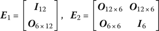
13.3.2.1 From Ground to Road Wheels (Elements 1–12)
The elements i![]() are those from the ground to the road wheels. According to the transfer matrix of a three‐dimensional spring (Equation (11.3)), the transfer matrices
are those from the ground to the road wheels. According to the transfer matrix of a three‐dimensional spring (Equation (11.3)), the transfer matrices ![]() can be obtained and the transfer equations of element i are
can be obtained and the transfer equations of element i are
By means of Equation (13.3), these 12 equations can be written as
where
13.3.2.2 Road Wheels (Elements 13–24)
According to the transfer matrix of a lumped mass vibrating in three‐dimensional space, the transfer matrices ![]() can be obtained, and the transfer equations of elements i
can be obtained, and the transfer equations of elements i![]() for the road wheels are
for the road wheels are
By means of Equation (13.3), these 12 equations can be written as
where

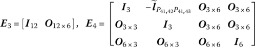
13.3.2.3 From Road Wheels to Hull (Elements 25–36)
Similar to section 13.3.2.1, the transfer equations of elements i![]() from the road wheels to the hull are
from the road wheels to the hull are
By means of Equation (13.3), these 12 transfer equations can be written as
where

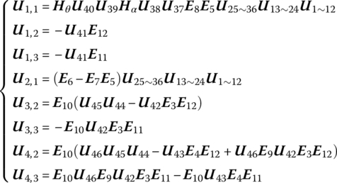
According to the form of ![]() in Equation (13.4), the 72 equations in Equation (13.16) can be divided into two parts. The first part is
in Equation (13.4), the 72 equations in Equation (13.16) can be divided into two parts. The first part is
where
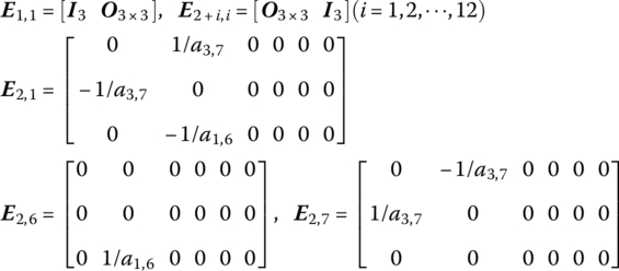
(a1,6, a2,6, a3,6) and (a1,7, a2,7, a3,7) are the coordinates of P37,31 and P37,32 at the body coordinate system fixed on body 37.
At point ![]() we have
we have
namely
There are 33 equations in Equation (13.20), and the 14th, 16th and 17th equations are already used in Equation (13.18). After removing these three equations, the other 30 equations are the second part of the 72 equations in Equation (13.16), that is
where
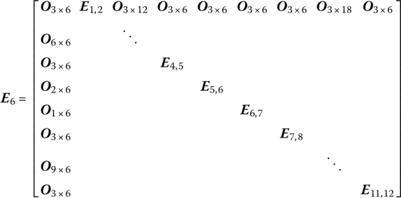
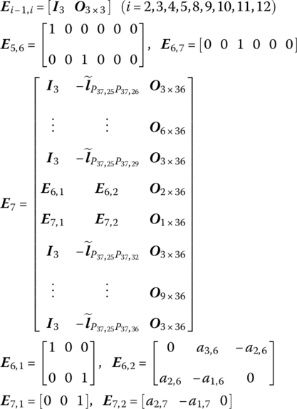
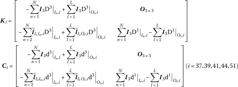
13.3.2.4 Hull (Element 37)
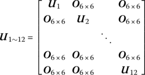
The hull is regarded as a rigid body with 12 input ends and one output end. According to the transfer matrix of a rigid body with N input ends and one output end (Equation (11.18)), the transfer matrix ![]() can be obtained, and the transfer equation of element 37 for the hull is
can be obtained, and the transfer equation of element 37 for the hull is
where

13.3.2.5 From Hull to Revolving Part (Element 38)
According to the transfer matrix of a spatial elastic joint, the transfer matrix ![]() of element 38 from the hull to the revolving part can be obtained. Considering the coordinate transform of the angle α between the hull and the revolving part, the transfer equation is
of element 38 from the hull to the revolving part can be obtained. Considering the coordinate transform of the angle α between the hull and the revolving part, the transfer equation is
where

![]() is the coordinate transform matrix corresponding to angle α.
is the coordinate transform matrix corresponding to angle α.
13.3.2.6 Revolving Part (Element 39)
According to the transfer matrix of a rigid body with one input end and one output end, the transfer matrix ![]() can be obtained, and the transfer equation of the revolving part is
can be obtained, and the transfer equation of the revolving part is
13.3.2.7 From Revolving Part to Pitching Part (Element 40)
Similar to section 13.3.2.5, the transfer equation from the revolving part to the pitching part is
where

![]() is the transfer matrix from the revolving part to the pitching part and
is the transfer matrix from the revolving part to the pitching part and ![]() is the coordinate transform matrix corresponding to the departure angle θ.
is the coordinate transform matrix corresponding to the departure angle θ.
13.3.2.8 Pitching Part (Element 41)
The pitching part is regarded as a rigid body with one input end and two output ends. According to the transfer matrix of a rigid body with one input end and L output ends, the transfer matrix ![]() can be obtained, and the transfer equation of the pitching part is
can be obtained, and the transfer equation of the pitching part is
13.3.2.9 Gun Breech and Muzzle Brake (Elements 44 and 51)
According to the transfer matrix of a rigid body with one input end and one output end, both the transfer matrix ![]() of the gun breech and the transfer matrix
of the gun breech and the transfer matrix ![]() of the muzzle brake can be obtained. Their transfer equations are
of the muzzle brake can be obtained. Their transfer equations are
13.3.2.10 Barrel (Six Elastic Beams, Elements 45–50)
According to the transfer matrix of a spatial vibrating beam, the transfer matrices U45, U46, U47, U48, U49 and U50 of six elastic beams can be determined, and the corresponding transfer equations are, respectively
where
![]() and
and ![]() are the transfer matrices of elements 42 and 43, respectively, which can be obtained through the transfer matrix of a spatial elastic joint.
are the transfer matrices of elements 42 and 43, respectively, which can be obtained through the transfer matrix of a spatial elastic joint.
At points P45,46 and P46,47, according to the geometric relation, we have
Let ![]() , and substituting Equation (13.7) into Equations (13.41) and (13.42), we obtain
, and substituting Equation (13.7) into Equations (13.41) and (13.42), we obtain
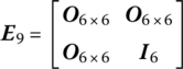
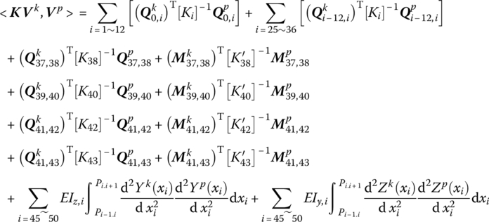
13.4 Overall Transfer Equation of the System
Substituting Equations (13.7), (13.31), (13.32) and (13.34)–(13.39) into Equation (13.33), we obtain
Let
Then
Substituting Equations (13.10), (13.13), (13.18), (13.24), (13.26), (13.28), (13.29) and (13.45) into Equation (13.31), substituting Equations (13.10), (13.13) and (13.18) into Equation (13.21), substituting Equations (13.32) and (13.45) into Equation (13.43), and substituting Equations (13.7), (13.32), (13.34) and (13.45) into Equation (13.44), we obtain
where
Equation (13.46) is the overall transfer equation of a self‐propelled artillery system and ![]() is the overall transfer matrix of the system.
is the overall transfer matrix of the system.
13.5 Vibration Characteristics of the System
It is important in the launch dynamics of self‐propelled artillery to compute the natural vibration characteristics exactly. There are two important features of the natural vibration characteristics of self‐propelled artillery: (1) the performance of self‐propelled artillery can be improved by adjusting the distribution of the natural frequencies of self‐propelled artillery and (2) they can provide indispensable modal parameters for analyzing the dynamic response of self‐propelled artillery with the modal method. The workload involved in computing the vibration characteristics of self‐propelled artillery with the transfer matrix method of multibody system is small, the computation speed is fast and the computation precision is high.
13.5.1 Eigenequation of a Self‐propelled Launch System
In Equation (13.46), ![]() is composed of the state vectors (
is composed of the state vectors (![]() ) at system boundary points. Half of the elements of the state vector at a boundary point are determined by the boundary conditions. For self‐propelled artillery, each state vector
) at system boundary points. Half of the elements of the state vector at a boundary point are determined by the boundary conditions. For self‐propelled artillery, each state vector ![]() between the 12 road wheels and the ground contains six elements, that is, the displacements and forces in three directions each, in which the three elements representing the displacement are always equal to 0. Thus, 36 elements of the 72 elements of
between the 12 road wheels and the ground contains six elements, that is, the displacements and forces in three directions each, in which the three elements representing the displacement are always equal to 0. Thus, 36 elements of the 72 elements of ![]() are 0. Let the symbol
are 0. Let the symbol ![]() represent the state vector that only includes the remnant elements after these 0 elements have been removed from
represent the state vector that only includes the remnant elements after these 0 elements have been removed from ![]() ; it therefore has 36 elements.
; it therefore has 36 elements. ![]() is the state vector at the boundary points of the gun breech and
is the state vector at the boundary points of the gun breech and ![]() is the state vector at the boundary points at the muzzle. Each of these contains 12 elements, including displacements, angle displacements, forces and moments in three directions each. Both the gun breech and muzzle are free of boundaries, therefore the six elements representing the forces and moments are always equal to 0. In the same way, let
is the state vector at the boundary points at the muzzle. Each of these contains 12 elements, including displacements, angle displacements, forces and moments in three directions each. Both the gun breech and muzzle are free of boundaries, therefore the six elements representing the forces and moments are always equal to 0. In the same way, let ![]() and
and ![]() represent the remnants after these 0 elements are removed from
represent the remnants after these 0 elements are removed from ![]() and
and ![]() , respectively, and each of them has six elements. In this case, there are 48 elements always equal to 0 in
, respectively, and each of them has six elements. In this case, there are 48 elements always equal to 0 in ![]() . Removing them from
. Removing them from ![]() leads to a new state vector
leads to a new state vector ![]() , which has 48 elements, that is
, which has 48 elements, that is
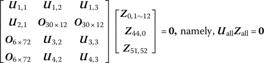
Deleting columns 1–3, 7–9, 13–15, 19–21, 25–27, 31–33, 37–39, 43–45, 49–51, 55–57, 61–63, 67–69, 79–84 and 91–96 in ![]() , a new matrix
, a new matrix ![]() with 48 orders can be obtained. Equation (13.46) can be written as
with 48 orders can be obtained. Equation (13.46) can be written as
The elements of ![]() and
and ![]() are only decided by the total parameters and eigenfrequencies of the system. When the total parameters are determined, Equation (13.49) should have a nontrivial solution for any eigenvalue of the system. Here, the determinant of
are only decided by the total parameters and eigenfrequencies of the system. When the total parameters are determined, Equation (13.49) should have a nontrivial solution for any eigenvalue of the system. Here, the determinant of ![]() should be zero
should be zero
Solving Equation (13.50), the eigenfrequencies of self‐propelled artillery, ![]() , can be obtained. The state vector
, can be obtained. The state vector ![]() corresponding to ωk can be evaluated by solving Equation (13.49). Of course,
corresponding to ωk can be evaluated by solving Equation (13.49). Of course, ![]() is also obtained, that is, the state vectors
is also obtained, that is, the state vectors ![]() corresponding to ωk are obtained. Based on these state vectors at the system boundary, through the transfer equation of each element one by one, all the state vectors in the system, including each connection point and an arbitrary point on the beam (gun tube), can be obtained. Thus, the vibration characteristics of self‐propelled artillery are obtained, which include the eigenfrequencies
corresponding to ωk are obtained. Based on these state vectors at the system boundary, through the transfer equation of each element one by one, all the state vectors in the system, including each connection point and an arbitrary point on the beam (gun tube), can be obtained. Thus, the vibration characteristics of self‐propelled artillery are obtained, which include the eigenfrequencies ![]() and the eigenvectors corresponding to each ωk, and the datum of eigenvectors are included in the elements of all state vectors of the system, which can be obtained by selecting them from state vectors.
and the eigenvectors corresponding to each ωk, and the datum of eigenvectors are included in the elements of all state vectors of the system, which can be obtained by selecting them from state vectors.
13.6 Dynamic Response of the System
13.6.1 Body Dynamic Equation of a Body Element and its Parameter Matrix
The body dynamic equations of the system can be obtained by combining the body dynamic equations of the elements
In this section, the body dynamic equations of self‐propelled artillery are established, and the augmented eigenvector of self‐propelled artillery, which automatically satisfies the orthogonality, is introduced.
Let the static equilibrium position of the artillery system before firing be the reference position. The force and the moment of the gravity acting on each element of the artillery system will not appear in the corresponding dynamic equation because they have been counteracted by the elastic force and the elastic moment produced by the static deformation of the corresponding spring and rotary spring. All the displacements and angle displacements involved in the elastic forces and elastic moments are measured from the static equilibrium position. This treatment not only leads to concise dynamic equations, but is also in good agreement with the real method of measuring the dynamic response of artillery in which the static equilibrium position of the artillery system is the benchmark.
13.6.1.1 Road Wheels (Elements 13–24)
A road wheel is a lumped mass with spatial vibration, and the parameter matrices of the road wheel i (i = 13, 14, …, 24) are
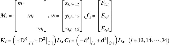
where mi, ![]() and
and ![]() are the mass of road wheel i, the coordinates of the column matrix of linear displacement with respect to the static equilibrium position and the coordinates of the column matrix of external force, respectively.
are the mass of road wheel i, the coordinates of the column matrix of linear displacement with respect to the static equilibrium position and the coordinates of the column matrix of external force, respectively.
13.6.1.2 Hull, Revolving Part, Pitching Part, Gun Breech, Muzzle Brake (Elements 37, 39, 41, 44 and 51)
The hull, revolving part, pitching part, gun breech and muzzle brake are all rigid bodies, and the parameter matrices of elements 37, 39, 41, 44 and 51 are
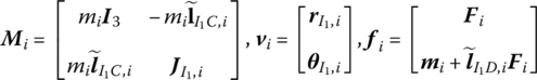
where mi is the mass of the rigid body i, I1 represents the first input end of the rigid body and C is the mass center of the rigid body. D represents the action point of external force, ![]() is the inertia moment matrix of rigid body i with respect to the first input end and
is the inertia moment matrix of rigid body i with respect to the first input end and ![]() is the linear displacement of the first input end with respect to equilibrium position.
is the linear displacement of the first input end with respect to equilibrium position. ![]() is the angle displacement of rigid body i,
is the angle displacement of rigid body i, ![]() and
and ![]() are column matrices of external force and external moment, and N and L are the total number of input and output ends, respectively.
are column matrices of external force and external moment, and N and L are the total number of input and output ends, respectively.
13.6.1.3 Barrel (Elements 45, 46, 47, 48, 49 and 50)
If the longitudinal and torsional deformations are neglected, that is, both longitudinal and rotation motion are rigid in the direction of the x axis of the beam, the parameter matrices of the six segments of the barrels numbered 45, 46, 47, 48, 49 and 50 are
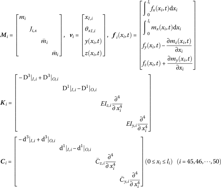
where xi are the coordinates of the point on beam i, li is the length of beam i, ![]() is the linear density of beam i, EI is bending stiffness, mi is the total mass,
is the linear density of beam i, EI is bending stiffness, mi is the total mass, ![]() , and Ji,x is the moment of inertia with respect to the axis of beam i.
, and Ji,x is the moment of inertia with respect to the axis of beam i.
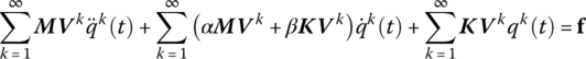
13.6.2 Body Dynamic Equations and the Augmented Eigenvector of the System
After the body dynamic equations of all body elements have been written according to the sequence number, the body dynamic equation of self‐propelled artillery can be written as follows:
where
where ![]() is the displacement column matrix of the system,
is the displacement column matrix of the system, ![]() and
and ![]() are augmented operators, and
are augmented operators, and ![]() is the damping augmented operator.
is the damping augmented operator. ![]() is the column matrix of external force and i is the sequence number of each body element.
is the column matrix of external force and i is the sequence number of each body element.
Let

Where
where k is mode rank, q(t) is generalized coordinates and ![]() is the augmented eigenvector of self‐propelled artillery.
is the augmented eigenvector of self‐propelled artillery.
According to the MSTMM, the augmented eigenvector ![]() satisfies the orthogonality automatically
satisfies the orthogonality automatically
where ![]() is the eigenfrequency of the system and Mp is the modal mass of the pth rank.
is the eigenfrequency of the system and Mp is the modal mass of the pth rank.
For proportional damping, the damping augmented operator ![]() is
is
where α and β are constant.
13.6.3 Validation of an Augmented Eigenvector Automatically Satisfying Orthogonality
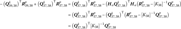
13.6.3.1  is Symmetric about Augmented Operator
Because ![]() are all real symmetric matrices, it is known from Equation (13.56) that
are all real symmetric matrices, it is known from Equation (13.56) that ![]() is also a real symmetric matrix, indicating that
is also a real symmetric matrix, indicating that ![]()
Thus, ![]() is symmetric about augmented operator
is symmetric about augmented operator ![]() .
.
13.6.3.2  is Symmetric about Augmented Operator
The following equations hold for the dynamics of the self‐propelled artillery weapon system:
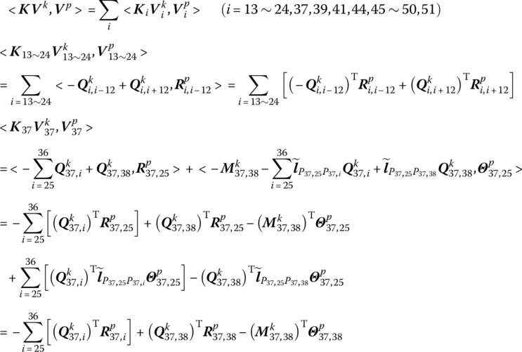
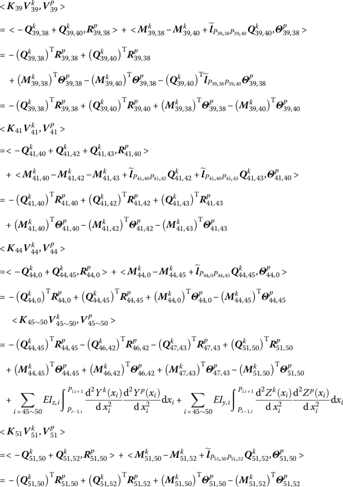
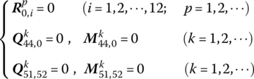
Note that the force and moment at both sides of the joint are equal and the boundary conditions are as follows:
Hence
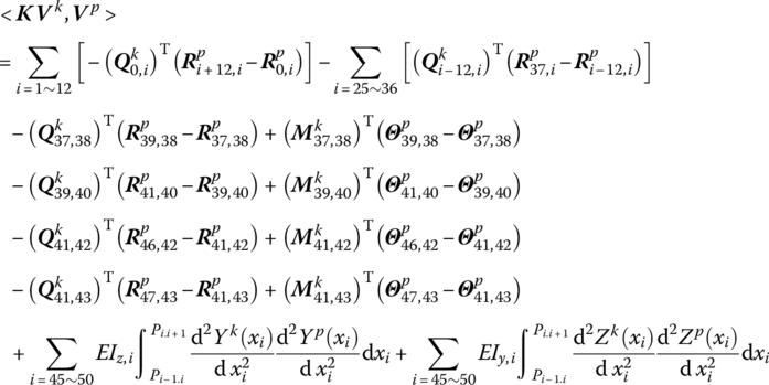
Let
There are relations between both sides of joint i in the following
namely
Thus, if both the departure angle and the azimuth angle are 0, that is, ![]() , then
, then
Considering the symmetry of matrices [K] and [K′], k and p on the right‐hand side of the above equation are exchangeable, so we have an equation as follows:
Thus, when ![]() ,
, ![]() is symmetric about augmented operator
is symmetric about augmented operator ![]() . If the departure angle and the azimuth angle are not 0, taking the term
. If the departure angle and the azimuth angle are not 0, taking the term ![]() as an example,
as an example, ![]() results in
results in ![]() and
and ![]() , but
, but
Considering ![]() , we have
, we have
Obviously, even if ![]() and
and ![]() , Equation (13.69) still is valid.
, Equation (13.69) still is valid.
In conclusion, ![]() is symmetric about augmented operators
is symmetric about augmented operators ![]() and
and ![]() . It is validated that the augmented eigenvector of self‐propelled artillery automatically satisfies the orthogonality.
. It is validated that the augmented eigenvector of self‐propelled artillery automatically satisfies the orthogonality.
13.6.4 Dynamic Response of the System
Substituting Equations (13.58) and (13.62) into Equation (13.55) gives
Taking the inner product to ![]() for both sides of Equation (13.106) yields
for both sides of Equation (13.106) yields
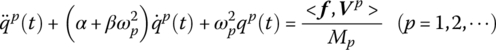
Substituting the column matrix of external force ![]() into Equation (13.107), we can obtain
into Equation (13.107), we can obtain ![]() by integration, and then the dynamic response of self‐propelled artillery can be obtained through Equation (13.58).
by integration, and then the dynamic response of self‐propelled artillery can be obtained through Equation (13.58).
Combining the generalized coordinate equations of self‐propelled artillery (Equation (13.107)), the launch dynamic equation of the projectile (Equation (13.70)) and the dynamic equations of interior ballistic two‐phase flow (Equations (13.73)–(13.105)), the launch dynamic equations of self‐propelled artillery can be determined. For the same moment, using the MacCormack format, the dynamic equations of interior ballistic two‐phase flow are solved, then, using the Runge–Kutta method, the body dynamic equations, as well as the launch dynamic equation of the projectile, are solved. After that, the dynamic parameters, including the dynamic response of the artillery and projectile motion in the gun tube, can be obtained. These are required to design, research and test for self‐propelled artillery.
13.7 Launch Dynamic Equations and Forces Analysis
The launch dynamic equations of a self‐propelled artillery system include the body dynamic equations of self‐propelled artillery, the launch dynamic equations of the projectile and the interior ballistic equation. The body dynamic equations of self‐propelled artillery were presented in section 13.4. Other dynamic equations are introduced in this section. The two‐phase flow dynamic model is adopted for interior ballistics.
13.7.1 Launch Dynamic Equation of a Projectile
The relevant coordinate systems are defined. The gun coordinate system ![]() is used to determine the orientation of the projectile with respect to the gun tube. The origin O3 is the intersection point between the axis of the gun tube and its vertical plane passing the mass center of the projectile, the
is used to determine the orientation of the projectile with respect to the gun tube. The origin O3 is the intersection point between the axis of the gun tube and its vertical plane passing the mass center of the projectile, the ![]() axis is directed toward the muzzle along the tangent of gun tube axis at O3, the y′ axis is in the plumb plane vertical with
axis is directed toward the muzzle along the tangent of gun tube axis at O3, the y′ axis is in the plumb plane vertical with ![]() axis and points up, and the
axis and points up, and the ![]() axis is determined by the right‐hand law.
axis is determined by the right‐hand law.
The projectile axis coordinate system O1ξ′η′ζ′ is used to determine the orientation of the projectile axis. The origin O1 is the geometrical center of the projectile (the intersection point between the cross‐section passing the mass center of the projectile and its geometrical longitudinal axis), the ξ′ axis is directed toward the head of the projectile along its geometrical longitudinal axis, the η′ axis is in the plumb plane vertical with ξ′ axis and points up, and the ζ′ axis is determined by the right‐hand law.
The motion of the projectile mass center is described in the gun coordinate system ![]() and the rotational motion of the projectile is described in the projectile axis coordinate system. It can be proved that the launch dynamic equations of a nonsymmetric projectile are [132]
and the rotational motion of the projectile is described in the projectile axis coordinate system. It can be proved that the launch dynamic equations of a nonsymmetric projectile are [132]
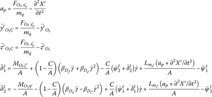
where
ap is the component of the acceleration of the projectile mass center along the gun axis with respect to the gun coordinate system ![]() . mq is the mass of the projectile. X′ is the recoil displacement of the gun.
. mq is the mass of the projectile. X′ is the recoil displacement of the gun. ![]() and
and ![]() are the vertical and lateral components of the projectile centroid displacement with respect to the gun coordinate system
are the vertical and lateral components of the projectile centroid displacement with respect to the gun coordinate system ![]() .
. ![]() and
and ![]() are the vertical and lateral components of displacement of O3.
are the vertical and lateral components of displacement of O3. ![]() ,
, ![]() and
and ![]() are the components of the force acting on the projectile along three coordinate axes at
are the components of the force acting on the projectile along three coordinate axes at ![]() .
. ![]() and
and ![]() are the components of external moment along the ξ′ and η′ axes, respectively. C is the polar moment of inertia of the projectile. A is the equatorial moment of inertia of the projectile. γ is the spinning angle of the projectile.
are the components of external moment along the ξ′ and η′ axes, respectively. C is the polar moment of inertia of the projectile. A is the equatorial moment of inertia of the projectile. γ is the spinning angle of the projectile. ![]() is the angle between the
is the angle between the ![]() axis and the projection of the projectile polar axis ξ′ on plane
axis and the projection of the projectile polar axis ξ′ on plane ![]() and is positive when the ξ′ axis is upside to the
and is positive when the ξ′ axis is upside to the ![]() axis.
axis. ![]() is the angle between the projectile polar axis ξ′ and the plane
is the angle between the projectile polar axis ξ′ and the plane ![]() and is positive when the ξ′ axis is on the right of
and is positive when the ξ′ axis is on the right of ![]() .
. ![]() is the angle between the x′ axis and the projection of the
is the angle between the x′ axis and the projection of the ![]() axis on plane x′O3y′ and is positive when the
axis on plane x′O3y′ and is positive when the ![]() axis is upside to the x′ axis.
axis is upside to the x′ axis. ![]() is the angle between the
is the angle between the ![]() axis and plane x′O3y′ and is positive when the
axis and plane x′O3y′ and is positive when the ![]() axis is on the right of x′O3y′.
axis is on the right of x′O3y′. ![]() and
and ![]() are projections of mass eccentricity along the η′ and ξ′ axes in projectile axis coordinate system O1ξ′η′ζ′, respectively.
are projections of mass eccentricity along the η′ and ξ′ axes in projectile axis coordinate system O1ξ′η′ζ′, respectively. ![]() and
and ![]() are components of mass eccentricity in the coordinate system fixed on the projectile.
are components of mass eccentricity in the coordinate system fixed on the projectile. ![]() and
and ![]() are projections of the dynamic unbalance along the η′ and ξ′ axes of projectile axis coordinate system O1ξ′η′ζ′.
are projections of the dynamic unbalance along the η′ and ξ′ axes of projectile axis coordinate system O1ξ′η′ζ′. ![]() and
and ![]() are the components of dynamic unbalance in the coordinate system fixed on the projectile.
are the components of dynamic unbalance in the coordinate system fixed on the projectile.
The piecewise rifling is expressed by
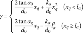
where α is the twist angle of rifling, lα is the position of the switch point between uniform and increasing twist rifling, ![]() , αg is the twist angle of rifling at the muzzle and α0 is the initial twist angle of rifling.
, αg is the twist angle of rifling at the muzzle and α0 is the initial twist angle of rifling.
13.7.2 Dynamic Equations of Interior Ballistic Two‐phase Flow
According to the dynamic model of interior ballistic two‐phase flow and basic hypotheses, basic equations of the main charge and central ignition tube are established using one‐dimensional gridding.
13.7.2.1 Basic Equations of Two‐phase Flow Dynamics for the Main Charge
Basic equations of the two‐phase flow dynamics for the main charge founded in Eulerian coordinates include the conservation equations of gas phase mass, gas phase momentum, gas phase energy, solid phase mass and solid phase momentum, namely

where A is the cross‐section area of the gun tube, ϕ is the porosity and ρg is the gas phase density. ug is the gas phase velocity, ![]() is the mass production rate of gas per unit bulk and
is the mass production rate of gas per unit bulk and ![]() is the mass flux of the gas source in the total bulk of a grid in the chamber. D is the drag force between two phases, P is the gas pressure and up is the solid phase velocity. eg is the internal energy of gas, Hc is the enthalpy per unit mass released by propellant burning and Hign is the enthalpy per unit mass brought by influent gas. Qs is the heat transfer between two phases and Rp is the stress within propellant grains.
is the mass flux of the gas source in the total bulk of a grid in the chamber. D is the drag force between two phases, P is the gas pressure and up is the solid phase velocity. eg is the internal energy of gas, Hc is the enthalpy per unit mass released by propellant burning and Hign is the enthalpy per unit mass brought by influent gas. Qs is the heat transfer between two phases and Rp is the stress within propellant grains.
In addition
where R is the gas constant, T is the gas temperature, γ is the gas adiabatic exponent and fp is the propellant force.
13.7.2.2 Basic Equations Group for the Central Ignition Tube
The basic equations for the central ignition tube founded in Eulerian coordinates include the conservation equations of gas phase mass, gas phase momentum and gas phase energy, namely
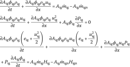
where Aig is the cross‐section area of the central ignition tube, ϕig is the porosity in the ignition tube and ρig is the gas phase density in the ignition tube. uig is the gas phase velocity, ![]() is the mass production rate per unit bulk produced by the ignition powder and
is the mass production rate per unit bulk produced by the ignition powder and ![]() is the mass flux out of the ignition tube. Pig is the gas pressure in the ignition tube, eig is the internal energy of the ignition gas, Hig is the enthalpy released by ignition powder burning and Hign is the enthalpy flowing out from the ignition tube. This yields
is the mass flux out of the ignition tube. Pig is the gas pressure in the ignition tube, eig is the internal energy of the ignition gas, Hig is the enthalpy released by ignition powder burning and Hign is the enthalpy flowing out from the ignition tube. This yields


where Rig is the ignition gas constant, γig is the adiabatic exponent of the ignition gas, Tig is the ignition gas temperature, fig is the propellant force of the ignition powder and T1,ig is the explosion temperature of the ignition powder.
13.7.2.3 Auxiliary Equations
- Nobel–Abel gas state equation(13.83)where α is the covolume of propellant gas, P is the gas pressure, ρg is the gas density, R is the gas constant and T is the gas temperature.
- Mass production rate of gas(13.84)
where ρp is the solid density, which is constant, and ψ is the relative burnt bulk of propellant.
The combustion of propellant obeys the geometric burning law
(13.85)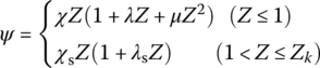 (13.86)
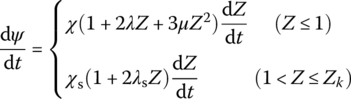
where χ, λ, μ, χs and λs are the characteristic quantities of propellant grain form and Z is the relative burnt thickness.
Burning rate obeys the exponential law, that is
(13.87)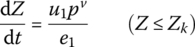
where e1 is half of the propellant web size, and u1 and v are the coefficient and exponent of burning rate, respectively.
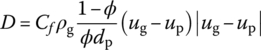
- Anderson formula for the drag force between two phases [273](13.88)where
 (13.89)
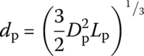 (13.90)
 (13.91)
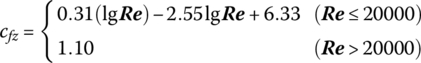 (13.92)
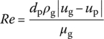 (13.93)where dp is the equivalent diameter of the propellant grain, Dp and Lp are the diameter and length of the propellant grain, ϕ0 is the critical porosity of the propellant with free loading, Re is the Reynolds number of gas motion calculated with the characteristic size that is the equivalent diameter dp, μg is the viscosity coefficient,
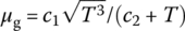
 and
and  .
. - Formula for stress within propellant grains [273]
Stress Rp is calculated through the following formula according to porosity ϕ
(13.94)
- Formula for heat transfer between two phases
Heat transfers from gas to solid, and the quantity of heat exchange per unit bulk is
(13.95)
where Ap is the surface area of the propellant grain, Tps is the surface temperature and ht is the coefficient of heat interchange. It should be noted that
(13.96) (13.97)
where ap is the coefficient of temperature conductivity of the propellant, kp is the coefficient of heat conductivity of the propellant, and hp and hre are the coefficients of convection heat transfer and radiative heat interchange, respectively. Note that
(13.98) (13.99)
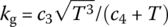 (13.100)
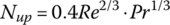 (13.101)
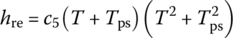
where kg is the coefficient of the heat conductivity of the gas, Nup is the Nusselt number and Pr is Planck’s constant. Commonly,
 ,
,  ,
,  ,
,  , εp is the superficial blackness
  , σ0 is the Stefan–Boltzmann constant and
  .
. - Formula for the mass flux of jet ejected from the primer
When the primer is fired, it produces hot gas and jet into the first grid of the ignition tube, and the jet can be regarded as the “source” of the grid. Because
 has been defined as “the mass flux out of the ignition tube in the total bulk of a grid” in Equation (13.78), the mass flux of the source is defined in the total bulk of the grid(13.102)
where
 is the mass flux of the jet form primer.
Taking a primer as an example, the test result of the mass flux of jet [273] is
(13.103)
- Formula for the mass flux of the ignition hole
The ignition gas out of the ignition tube from the ignition hole is regarded as the “source” in a grid, and the mass flux of excurrent gas is
(13.104)
where nig is the total number of ignition holes in one grid (when ignition holes are not broken
 ),
),  is the mass flux of the ignition hole, η is the flux coefficient, Sk is the area of the ignition hole and Pout is the pressure out of the ignition tube.
13.7.3 Analysis for the Force Acting on a Self‐propelled Launch System
During the launch process, the forces acting on self‐propelled artillery are mainly the interaction forces between the gun barrel and the pitching part, the pitching part and the revolving part, the revolving part and the hull, the hull and the road wheels, and the road wheels and the ground. All these forces and moments are regarded as the internal forces of the system. The recoil resistance produced by the recoil and counterrecoil mechanism is decomposed into two parts: the internal force and the external force. The internal force is proportional to the relative displacement between the barrel and the pitching part. The force of the propellant gas, the Bourdon force, the force acting on the barrel by the projectile and the tensile force of the pedrail are external forces.
The forces acting on the projectile in the gun tube are very complex and include gravity, the pressure of the propellant gas, the air resistance acting on the head of the projectile, the contact force between the rotating band and the wall of the gun tube, the contact force between the bourrelet and the wall of the gun tube, and the corresponding moment.
The forces acting on the projectile are described in the form of column matrices in gun coordinate system ![]() , and the corresponding moments acting on the projectile are described in the form of column matrices in projectile axis coordinate system O1ξ′η′ζ′. The detailed analysis processes and expressions of all the forces can be found in reference [132]. All external forces acting on the artillery are expressed in the corresponding inertia coordinate which corresponds to each element, and the column matrix
, and the corresponding moments acting on the projectile are described in the form of column matrices in projectile axis coordinate system O1ξ′η′ζ′. The detailed analysis processes and expressions of all the forces can be found in reference [132]. All external forces acting on the artillery are expressed in the corresponding inertia coordinate which corresponds to each element, and the column matrix ![]() of external forces in the body dynamic equation of each element can be evaluated. The column matrix
of external forces in the body dynamic equation of each element can be evaluated. The column matrix ![]() of the external forces of the system is obtained according to the form of Equation (13.57). The computation methods of the force acting on the artillery by the propellant gas, the Burdon force and the force acting on the barrel by the projectile, the force acting on the barrel and pitching part by the recoil and counterrecoil mechanism, and the tensile force of the pedrail can be found in references [132], and [274–277], respectively.
of the external forces of the system is obtained according to the form of Equation (13.57). The computation methods of the force acting on the artillery by the propellant gas, the Burdon force and the force acting on the barrel by the projectile, the force acting on the barrel and pitching part by the recoil and counterrecoil mechanism, and the tensile force of the pedrail can be found in references [132], and [274–277], respectively.
13.8 Dynamics Simulation of the System and its Test Verifying
13.8.1 Launch Dynamics Simulation System of Self‐Propelled Artillery
The launch dynamics simulation system of self‐propelled artillery is based on the MSTMM. The program for computing the launch dynamics of self‐propelled artillery is written in FORTRAN. The launch process of self‐propelled artillery with the initial disturbance is simulated under the condition of 0° departure angle and 0° azimuth angle. The vibration characteristics, the interior ballistic, the motion of the projectile in the gun tube and the dynamic response of artillery are computed. Some tests have been carried out and their results verify the simulation system. Some results of simulation and testing are given below.
13.8.2 Simulation and Test Verifying for Vibration Characteristics
Natural vibration characteristics of self‐propelled artillery are simulated using the MSTMM according to the 0° departure angle and 0° azimuth angle. The modal parameters and the vibration characteristics are obtained via the experimental modal analysis of self‐propelled artillery. The simulation and test results of eigenfrequencies for the first 16 ranks are given in Table 13.1 and it can be seen that the simulation results are in good agreement with the test results.
Table 13.1 Simulation and test results of eigenfrequencies
| Mode rank, k | ωk/(rad/s) | Relative error/% | Mode rank, k | ωk/(rad/s) | Relative error/% | ||
| Simulation | Test | Simulation | Test | ||||
| 1 | 3.02 | — | — | 9 | 87.7 | 82.1 | 6.82 |
| 2 | 15.2 | 15.5 | −1.94 | 10 | 94.5 | — | — |
| 3 | 18.5 | 18.7 | −1.07 | 11 | 101.1 | 105.5 | −4.17 |
| 4 | 28.9 | 29.9 | −3.34 | 12 | — | 128.4 | — |
| 5 | 44.3 | 42.2 | 4.98 | 13 | 141.3 | 136.3 | 3.67 |
| 6 | 46.5 | 49.8 | −6.63 | 14 | 215.1 | 202.9 | 6.01 |
| 7 | 64.9 | — | — | 15 | 226.6 | 229.2 | –1.13 |
| 8 | 75.6 | — | — | 16 | 243.4 | 244.4 | –0.41 |
Some of simulation results of mode shapes are shown in Figures 13.4–13.7, in which the abscissas denote the sequence numbers of points, and the corresponding relation between the position of the point and the sequence number is shown in Table 13.2. The first rank mode represents the recoil motion of the barrel, and the second one represents the horizontal revolving motions of the turret, cradle and barrel. The third mode represents the pitching motions of the cradle and barrel, and the 16th mode represents the transverse motion of the barrel and complex motions of other elements. The low rank mode shapes do not represent the transverse elastic deformation of the barrel and such transverse elastic deformation can only be observed in higher rank mode shapes.
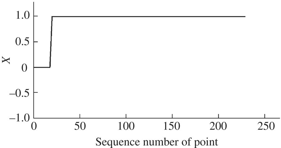
Figure 13.4 The first mode shape in the x direction.
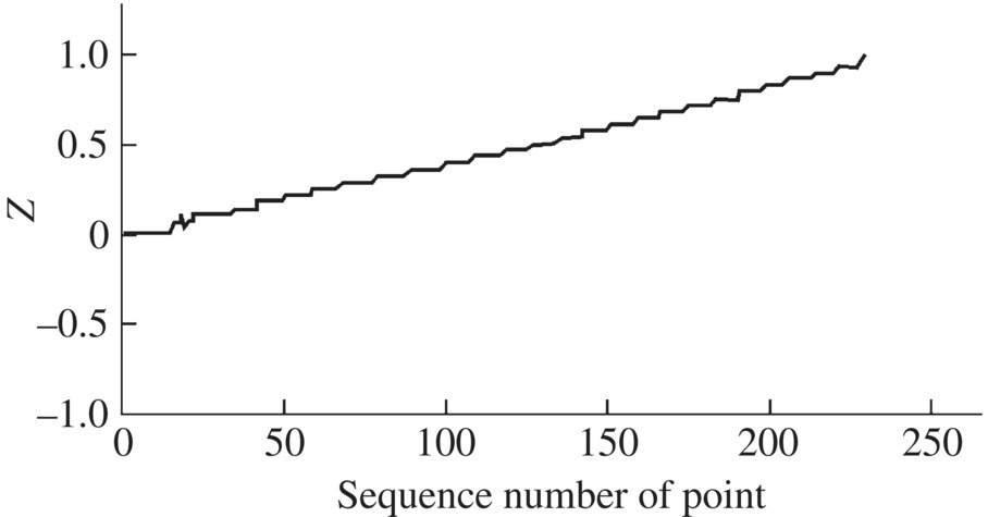
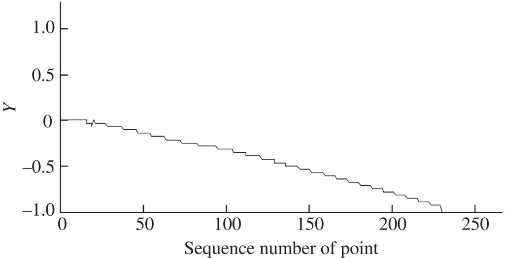

Figure 13.7 The 16th mode shape in the y direction.
Table 13.2 Corresponding relation between the position of point and the sequence number
| Sequence number | 1 | 2–13 | 14 | 15 | 16 | 17 | 18 | |
| Position | Ground |
|
P37,25 | P37,38 | P39,38 | P39,40 | P41,40 | |
| Sequence number | 19 | 20 | 21 | 22–29 | 30 | 31–68 | 69 | |
| Position | P41,42 | P44,0 | P44,45 | Element 45 (beam 1) |
P45,46 | Element 46 (beam 2) |
P46,47 | |
| Sequence number | 70–104 | 105–126 | 127–148 | 149–229 | 230 | |||
| Position | Element 47 (beam 3) |
Element 48 (beam 4) |
Element 49 (beam 5) |
Element 50 (beam 6) |
P51,52 | |||
13.8.3 Simulation and Test Verifying for Interior Ballistic Two‐phase Flow Dynamics
Simulation results of interior ballistic two‐phase flow dynamics and some experiment results are shown in Figures 13.8–13.12. These results play an important role in interior ballistic design.

Figure 13.8 Simulation and test results of breech pressure vs time.
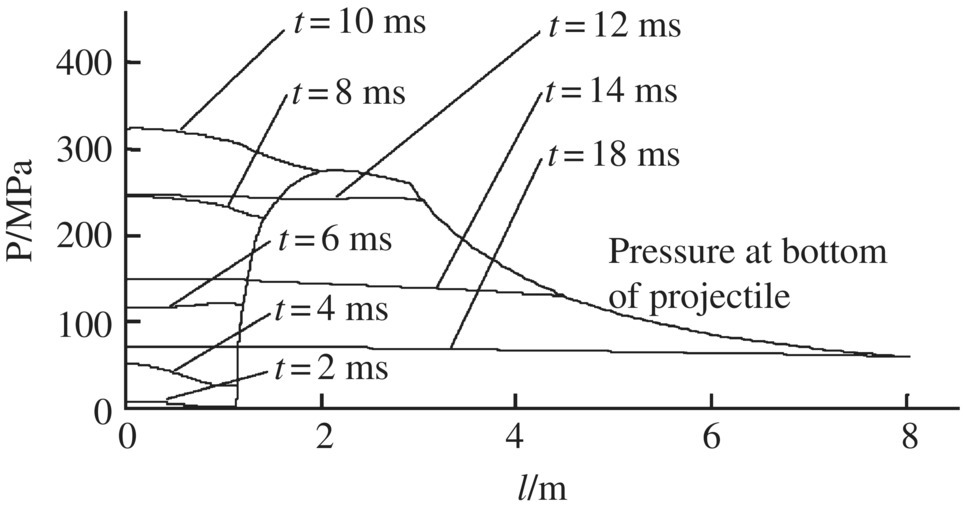
Figure 13.9 Gas pressure distribution.
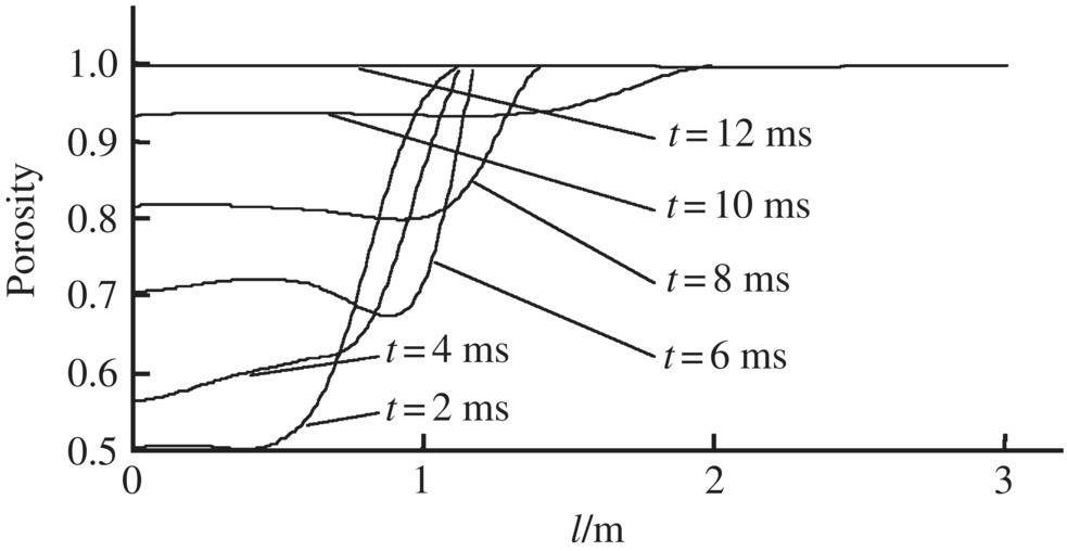
Figure 13.10 Porosity distribution.
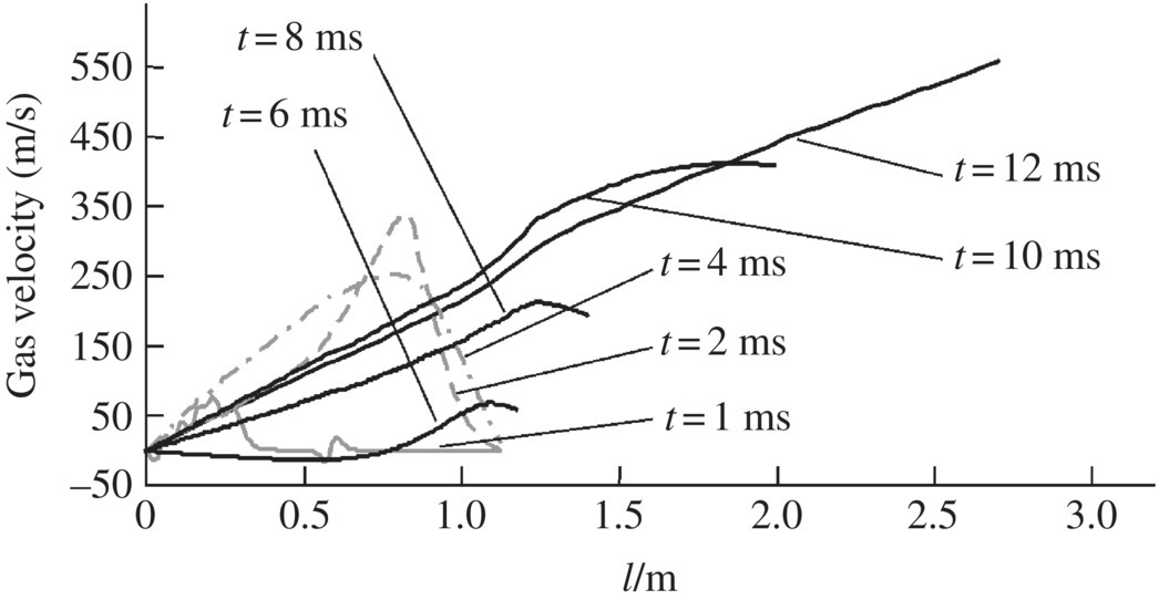
Figure 13.11 Gas velocity distribution.
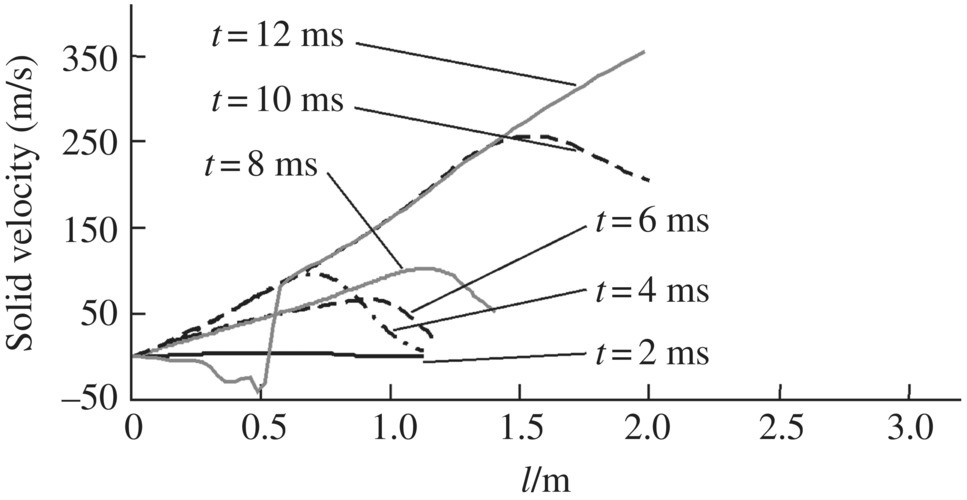
Figure 13.12 Solid velocity distribution.
The simulation and test results of the time‐history of the breech pressure are shown in Figure 13.8, and the simulation and test results of interior ballistic performances are shown in Table 13.3. The simulation and test results have good agreement, which demonstrates the accuracy of the simulation system. The simulation results of gas pressure distribution behind the projectile and its change over time are shown in Figure 13.9. The simulation results of porosity distribution behind the projectile and its change over time are shown in Figure 13.10. The simulation results of gas velocity distribution behind the projectile and its change over time are shown in Figure 13.11. The simulation results of solid velocity distribution behind the projectile and its change over time are shown in Figure 13.12.
Table 13.3 Simulation and test results of interior ballistic performances
| Maximal pressure at breech/MPa | Muzzle velocity of projectile/(m/s) | |
| Simulation | 330.6 | 928.2 |
| Test | 327.4 | 931.0 |
13.8.4 Simulation and Test Verifying for the Dynamic Response of the System
The simulation results of the dynamic response of self‐propelled artillery and some test results are shown in Figures 13.13–13.16. These results are an important foundation for the design and performance evaluation of artillery. Time‐history simulations of the resultant force acting on the barrel, recoil resistances, recoil and muzzle displacements with their test results are presented in Figures 13.13–13.16. Some simulation and test results are in good agreement.

Figure 13.13 Resultant force of barrel.


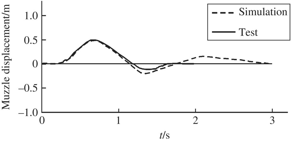
Figure 13.16 Muzzle displacement.
13.8.5 Simulation and Test Verifying for Projectile Launch Dynamics
The simulation results of the launch dynamics of projectiles are shown in Figure 13.17–13.26. These results provide a necessary ballistic environment for design and failure diagnosis of the mechanism carried by the projectile, such as fuze, and provide an important foundation for performance evaluation and design improvement of the projectile.

Figure 13.17 Spinning velocity of a projectile.
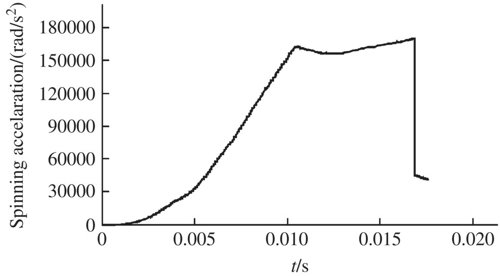

Figure 13.19 Acceleration of a projectile.
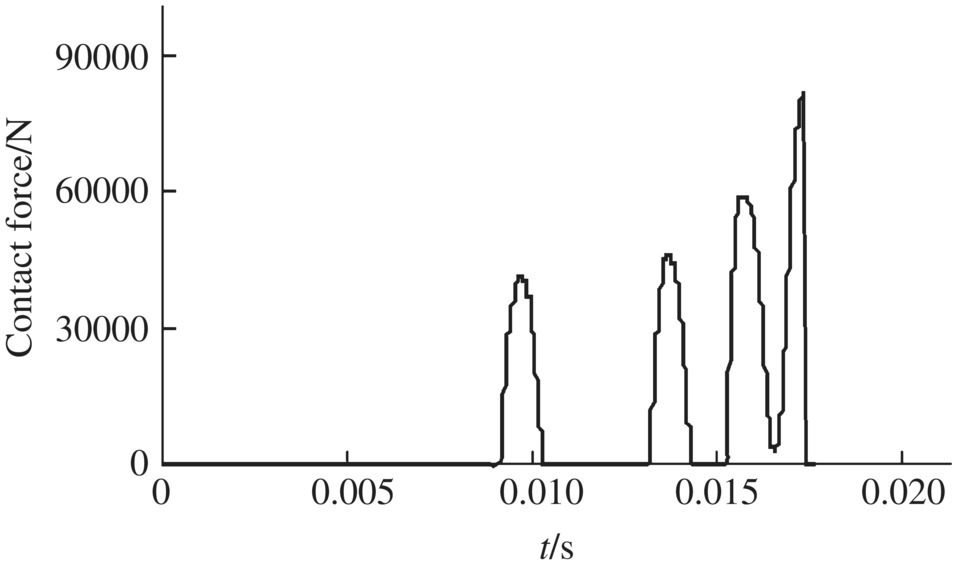
Figure 13.20 Contact force of a front bourrelet.
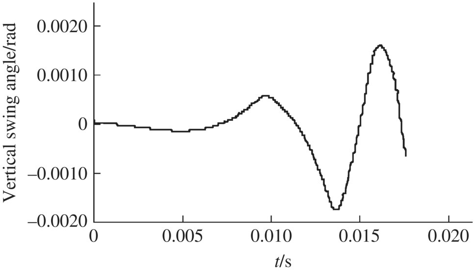
Figure 13.21 Vertical swing angle.
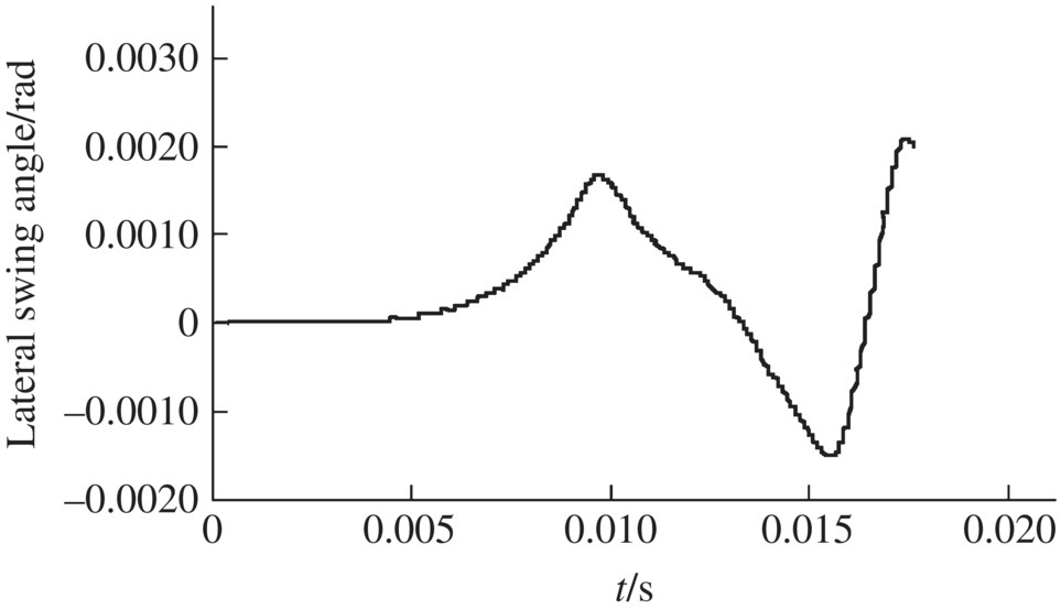
Figure 13.22 Lateral swing angle.

Figure 13.23 Amplitude swing angle.
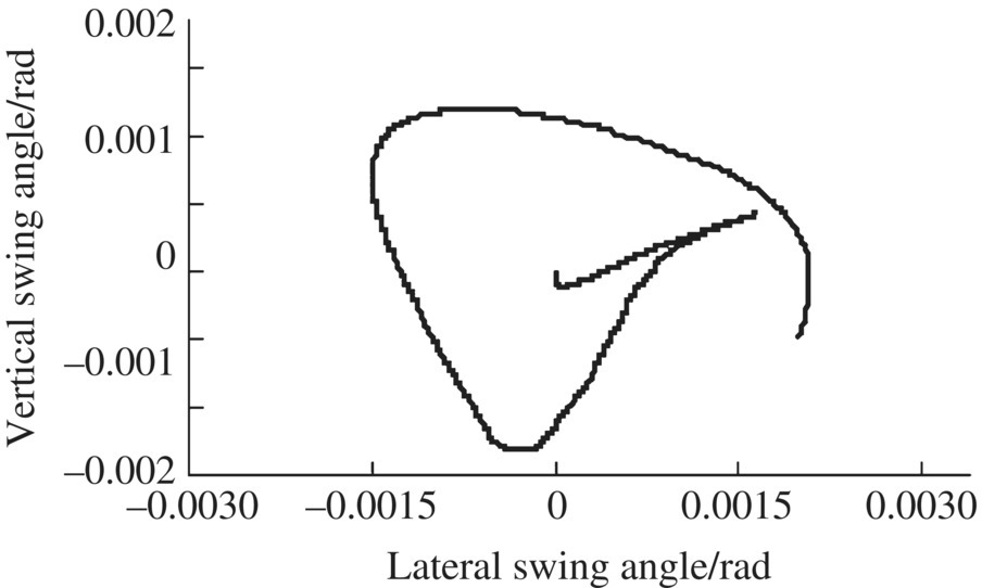
Figure 13.24 Track of swing angle.

Figure 13.25 Vertical swing angular velocity.
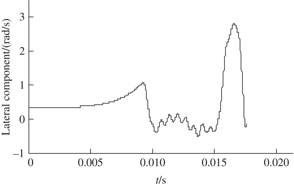
Figure 13.26 Lateral swing angular velocity.
The simulation results of the time‐history of projectile spinning velocity, spinning and longitudinal accelerations are shown in Figures 13.17–13.19. The simulation results of the contact force between the front bourrelet and the wall of the gun tube are shown in Figure 13.20. The time‐history results of the vertical and lateral swing angle of the projectile are illustrated in Figures 13.21 and 13.22. The time‐history result of the amplitude swing angle of the projectile is illustrated in Figure 13.23. The simulation result of the track of the swing angle of the projectile axis is shown in Figure 13.24. The simulation results of the vertical and lateral swing angular velocities of the projectile are shown in Figures 13.25 and 13.26.
13.8.6 Computation of the Initial Disturbance of the Projectile
The initial disturbance of the projectile includes the initial deflection angle ![]() , the initial swing angle
, the initial swing angle ![]() , the initial attack angle
, the initial attack angle ![]() and the angular velocity
and the angular velocity ![]() ,
, ![]() ,
, ![]() at the end time of the launch period. It also includes the initial coordinates, initial velocity, initial spinning angle and initial spinning velocity. When the projectile leaves the muzzle, the initial deflection angle
at the end time of the launch period. It also includes the initial coordinates, initial velocity, initial spinning angle and initial spinning velocity. When the projectile leaves the muzzle, the initial deflection angle ![]() when projectile begins to fly is the angle between the speed vector of the projectile mass center and the line of sight, that is
when projectile begins to fly is the angle between the speed vector of the projectile mass center and the line of sight, that is
where ![]() and
and ![]() are the vertical and lateral components of the muzzle speed, respectively, when the projectile is just flying off from the muzzle. At the same moment
are the vertical and lateral components of the muzzle speed, respectively, when the projectile is just flying off from the muzzle. At the same moment ![]() and
and ![]() are the vertical and lateral components, respectively, of the projectile mass center speed relative to the barrel axis and vg is the axial component of projectile speed relative to the gun tube.
are the vertical and lateral components, respectively, of the projectile mass center speed relative to the barrel axis and vg is the axial component of projectile speed relative to the gun tube.
If we differentiate Equation (13.108) with respect to time, the initial deflection angular velocity of projectile flight ![]() can be obtained:
can be obtained:
where ![]() and
and ![]() are the vertical and lateral components of the muzzle acceleration, respectively,
are the vertical and lateral components of the muzzle acceleration, respectively, ![]() and
and ![]() are the vertical and lateral components of the acceleration of the center of mass of the projectile relative to the barrel axis and ag is the axial component of acceleration of the center of mass of the projectile relative to the gun tube.
are the vertical and lateral components of the acceleration of the center of mass of the projectile relative to the barrel axis and ag is the axial component of acceleration of the center of mass of the projectile relative to the gun tube.
The initial swing angle of projectile ![]() is the angle between the projectile axis and the line of sight at the moment the projectile flies off the muzzle, that is
is the angle between the projectile axis and the line of sight at the moment the projectile flies off the muzzle, that is
where ![]() and
and ![]() are the vertical and lateral components of the angle between the projectile axis and the tangent of the barrel axis of the muzzle while the projectile is just flying off the muzzle.
are the vertical and lateral components of the angle between the projectile axis and the tangent of the barrel axis of the muzzle while the projectile is just flying off the muzzle. ![]() and
and ![]() are the vertical and lateral components of the angle between the tangent of the barrel axis at the muzzle and the line of sight at the same moment. These variables and their first partial derivatives with respect to time can be obtained after the projectile motion and artillery dynamic response are obtained through solving the launch dynamic equations of the system.
are the vertical and lateral components of the angle between the tangent of the barrel axis at the muzzle and the line of sight at the same moment. These variables and their first partial derivatives with respect to time can be obtained after the projectile motion and artillery dynamic response are obtained through solving the launch dynamic equations of the system.
The initial attack angle and its angular velocity when the projectile flies off the muzzle is
The simulation results of the initial disturbance of a round of projectiles are shown in Table 13.4.
Table 13.4 Simulation results of initial disturbance of projectile
| Initial disturbance | Vertical component | Lateral component |
| Deflection angle/(10−3rad) | –0.2193 | –0.0621 |
| Swing angle/(10−3rad) | –0.5071 | 1.9894 |
| Swing angle velocity/(rad/s) | –2.5851 | –0.5468 |
13.8.7 Simulation Result and Test Verifying for Firing Dispersion
Using the six degrees of freedom rigid body ballistic model and considering the effects on the flight process of the projectile produced by random factors such as the deviation of projectile mass, mass eccentricity, dynamic unbalance and wind synthetically, the flight dynamic equation of the projectile is established. On the basis of the launch dynamics of self‐propelled artillery based on the MSTMM, the simulation system for launch and flight dynamics is established and the simulations for launch and flight dynamics are achieved. Using Monte Carlo simulation technology and taking account of random variables such as the mass of the projectile, the mass of the propellant, the burning rate, the gap between the projectile and the barrel, the moment of inertia of the projectile, mass eccentricity, dynamic unbalance and wind speed, many simulation times for launch and flight dynamics are obtained, as well as the simulation results for the firing dispersion of a self‐propelled artillery system.
According to the static measurement data in the firing dispersion test of self‐propelled artillery, using the method mentioned above, the vertical target dispersion and ground dispersion can be simulated. These results can be used to discuss the influence of random factors on firing dispersion, and to analyze the measures for improving the firing dispersion of weapon systems. The simulation is carried out by adopting the same parameters of the experiment, such as the mean values and the variances of the mass eccentricity, dynamic unbalance, projectile/barrel clearance and propellant mass, etc. 200 and 100 rounds are simulated to evaluate the vertical target dispersion at 1000 m, and the ground dispersion at a maximum range of the self‐propelled artillery, respectively. The simulation result of target impact dispersion is shown in Figure 13.27. The simulation results of target impact dispersion and firing dispersion are in good agreement with the test results (the detailed data are omitted), which shows that the theory of launch dynamics based on MSTMM can provide important technology support to improve the firing precision and other dynamic performance for self‐propelled artillery.
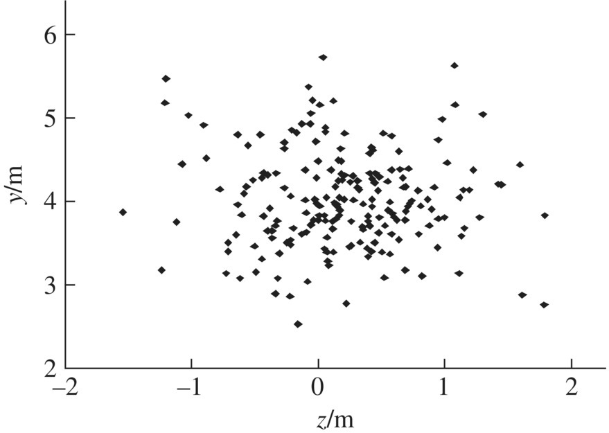
Figure 13.27 Simulation result of target impact dispersion.