
3
Augmented Eigenvector and System Response
3.1 Introduction
By presenting the new concepts of the body dynamics equation of the body element and the body dynamics equations of a system in the transfer matrix method for multibody systems (MSTMM), the complicated global dynamics equation of a system is no longer needed in solving multiple rocket launch system dynamics (MRLSD). The body dynamics equations of a system are merely the assemblage of the body dynamics equations of the body elements of the system, which are totally different from the global dynamic equations of the system. It is also not necessary to consider the connection relations among body elements of the system because they have been considered in the overall transfer matrix and vibration characteristics of the system. There are uniform forms of body dynamics equations for various body elements, therefore there are very simple forms of body dynamics equations of systems for multi‐rigid‐flexible‐body systems (MRFSs). These make the writing and derivation of dynamics equations and solving the dynamics response more convenient.
The orthogonality of eigenvectors of MRFSs is the pre‐condition to calculate the dynamics response of the system accurately and makes the dynamics response quickly converge to the precision required by engineering in limited modals. For example, to assess scientifically and improve the performance of weapon systems, and to greatly reduce the consumption of ammunition in the test and realize the dynamics design of a weapons system, it is necessary to compute the vibration characteristics of the launch system and analyze precisely the dynamics response of the weapons system. However, the eigenvectors do not possess conventional orthogonality because of nonself‐conjugation of the eigenvalues of the MRFS caused by the dynamic coupling between the rigid and flexible bodies of the system. It is therefore difficult to precisely analyze the dynamics response of the system using the modal analysis method. Finding the orthogonal eigenvectors of a complex MRFS became a worldwide complex problem except for several special and simple dynamics models [230, 234].
To solve the problems of the orthogonality of eigenvectors and accurate analyses of the dynamics response of MRFSs, new concepts such as the body dynamics equation, augmented eigenvector and augmented operator of MRFSs were proposed (section 3.4), and it has been shown by the authors that the orthogonality of augmented eigenvectors can be satisfied automatically [4, 50, 55–63]. Exact analysis of the dynamics responses for linear MRFSs are also realized. These provide the basic theory and approach for solving systematically the problems of linear multibody system dynamics (MSD). The augmented eigenvector can be obtained by successively writing the modal coordinates of the corresponding displacements and angular displacements of body elements. It contains discrete and continuous variables. Its number of variables is equal to the number of body dynamics equations of the system. Its construction process is simple, convenient and programmable. These are important features of augmented eigenvectors which are different from ordinary eigenvectors. Using the orthogonality of augmented eigenvectors and the vibration characteristics of the system, the body dynamics equations of body elements, which cannot be solved directly, can be solved by translating them into the differential equations of motion independent to each other under principal coordinates. This ensures the very high computational speed of multi‐rigid‐flexible‐body systems dynamics (MRFSD).
The following topics are introduced in this chapter: the basic theory of the orthogonality of eigenvectors, new concepts such as the body dynamics equation, the augmented eigenvector and the augmented operator of MRFSs, verification of the orthogonality of augmented eigenvectors, which is satisfied automatically, solving the transient responses of MRFSs to any excitations using augmented eigenvectors [60–63], and solving steady‐state and static responses of MRFSs.
3.2 Body Dynamics Equation and Parameter Matrices
3.2.1 Body Dynamics Equation of Body Elements
Any multibody system (MS) may be composed of body elements such as lumped masses, rigid bodies, flexible bodies and others connected by various hinges. It can be shown that the dynamics equation of any body element i can be written in the matrix form
Equation (3.1) is the body dynamics equation, which is originally presented in the MSTMM, where, Mi, Ci, Ki, vi and fi are the parameter matrices of body element i. Mi is the parameter matrix of mass and denotes the mass distribution of the body element. vi is a column matrix composed of displacements and angular displacements indicating the motion state of the body element. The subscript t denotes differentiation with respect to time. Ki is the parameter matrix of stiffness and denotes all internal forces acting on the body elements and their points of action except the damping forces and damping torque when it acts on vi. Ci is the parameter matrix of damping and denotes the damping forces and damping torques acting on the body elements and their points of action when it acts on vi,t. fi is the column matrix of external forces and external torques acting on the body element.
If the damping forces are included in the external forces, Equation (3.1) can be written as
The body dynamics equations and the parameter matrices of typical body elements, such as lumped masses, rigid bodies and elastic bodies, are discussed in the following sections.
3.2.2 Parameter Matrices of Typical Elements
3.2.2.1 Parameter Matrix of a Lumped Mass Vibrating in Space
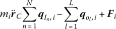
The body dynamics equation of a lumped mass vibrating in space is
where
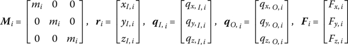
mi is the mass of lumped mass i, qI,i and qO, i are the column matrices of internal force acting on the input end I and output end O, and Fi is the column matrix of external force acting on the lumped mass i.
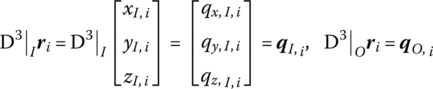
A linear operator D3 is defined as
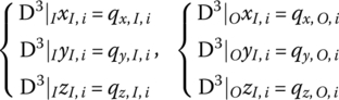
The physical meaning of the operator D3 is that the action of D3 on the displacement of a connection point of the system results in corresponding internal forces at the connection point except the damping force, that is
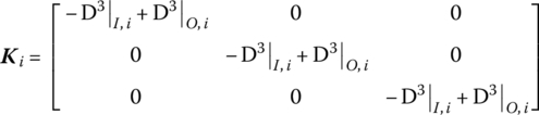
Using the linear operator, D3, Equation (3.3) can be reformed as Equation (3.2), where the detailed parameter matrices are

3.2.2.2 Parameter Matrix of a Rigid Body Vibrating in Space
For a rigid body i vibrating in space with N input and L output ends, the motion can be described by linear displacements ![]() and angular displacements
and angular displacements ![]() of the first input end I1 The motion equation of the mass center of the rigid body is
of the first input end I1 The motion equation of the mass center of the rigid body is
The rotation equation of the rigid body rotating about I1 is

where mi is the external principal moment acting on the rigid body, Fi is the principal vector of external force (contains the damping force) acting on the rigid body and ![]() is the moment of the principal vector of external force with respect to point I1.
is the moment of the principal vector of external force with respect to point I1.![]() is the internal moment of the nth input end of the rigid body,
is the internal moment of the nth input end of the rigid body, ![]() is the internal moment of the lth output end of the rigid body and
is the internal moment of the lth output end of the rigid body and ![]() is the moment of inertia matrix of the rigid body with respect to point I1.D is the simplified center of external force (center of moment).
is the moment of inertia matrix of the rigid body with respect to point I1.D is the simplified center of external force (center of moment).
The displacement of the mass center is
The acceleration of the mass center is
Substituting Equation (3.11) into Equation (3.8), we obtain
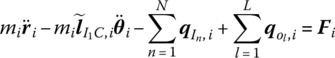
Rewriting Equation (3.9) yields

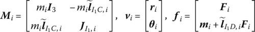
Combining Equations (3.12) and (3.13) and rewriting the body dynamics equation in the form of Equation (3.2) yields the parameter matrices

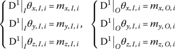
where D1 is a linear operator that denotes all internal moments of the body element at the connection point except the damping force, in which case it acts on the angular displacement of this point, namely
3.2.2.3 Parameter Matrix of a Beam Undergoing Transversal, Longitudinal and Torsional Vibrations
It can be shown that the dynamics equations for an Euler–Bernoulli beam with uniform cross‐section undergoing transversal, longitudinal and torsional vibrations are

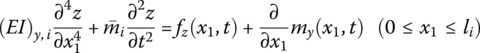

where y(x1, t), z(x1, t) and x(x1, t) denote the transverse and longitudinal displacements of any point on the beam relative to its equilibrium position, respectively. θx(x1, t) is the torsion angle of an arbitrary cross‐section on the beam relative to its equilibrium position. fx(x1, t), fv(x1, t) and fz(x1, t) denote the components of an external distributional force on the beam in the x, y and z directions, respectively. mx(x1, t), my(x1, t) and mz(x1, t) are the components of an external distributed moment on the beam in the x, yand z directions, respectively.
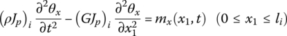
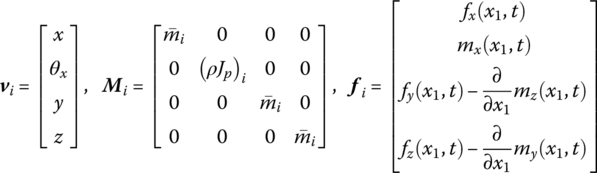
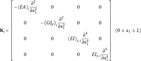
The parameter matrices of the beam with transverse, longitudinal and torsional vibration simultaneously can be obtained by combining Equations (3.16) to (3.19) and writing them in the form of Equation (3.2):
3.3 Basic Theory of the Orthogonality of Eigenvectors
3.3.1 Inner Product Space
3.3.2 Conjugate Transformation and Symmetric Transformation
3.4 Augmented Eigenvectors and their Orthogonality
In this section the new concept of augmented eigenvectors of MSs and their construction methods is introduced and it is verified that they satisfy orthogonality automatically.
3.4.1 Augmented Eigenvectors
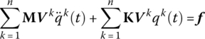
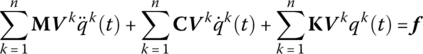
The uniform expression of the body dynamics equation for any body element in a MS without considering damping forces is
and the uniform expression of the body dynamics equation of the MS is
where

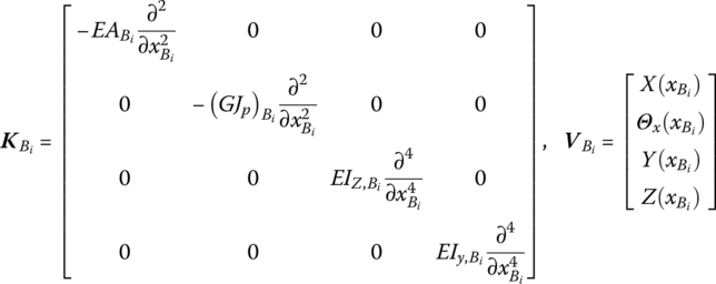
M and K are augmented operators presented originally in MSTMM, v is the column matrix of the displacement coordinates of the system, f is the column matrix of the external force of the system, the subscripts B1, B2, … and Bn are the sequence numbers of the body elements, and ![]() ,
, ![]() ,
, ![]() and
and ![]() are the parameter matrices of body element Bi.
are the parameter matrices of body element Bi.
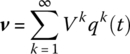
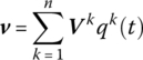
A new concept of augmented eigenvector V of the MS is defined as the column matrix of the modal coordinate corresponding to displacement coordinates of the MS:
The augmented eigenvectors Vk include the modal coordinates of displacements and angular displacements of each discrete element and the mode shape of each continuous element corresponding to the kth eigenfrequency ωk of the system.
Applying modal technology, assume that
where qk(t) is a generalized coordinate and the superscript k is the modal order.
The eigenvector covers only discrete variables for a discrete system or continuous functions for a continuous system. The two variables are included in the augmented eigenvector of a MRFS to describe discrete elements and continuous elements. They are different from the ordinary eigenfunctions of a continuous system and the eigenvectors of a discrete system. The eigenvetors for a discrete system consist only of discrete variables, while those for a continuous system consist only of continuous functions. However, both the discrete variables and the continuous functions should be included in the eigenvetors for a multi‐rigid‐flexible‐body system which consists of discrete elements (rigid bodies) and continuous elements (flexible bodies) at the same time, and such an eigenvector is called the augumented eigenvector in this book. The eigenvetors for a discrete system, as well as those for a continuous system, are just special cases of the augumented eigenvector of a general MRFS. Substituting Equation (3.39) into Equation (3.37) yields
For free vibration, namely ![]() ,
,

Figure 3.1 An MRFS vibrating in a plane.
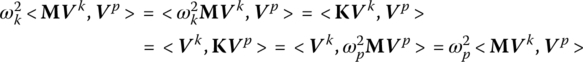
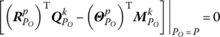
3.4.2 Orthogonality of Augmented Eigenvectors
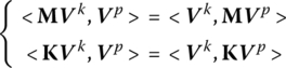
The orthogonality of the augmented eigenvectors ![]() with respect to M and K indicates that
with respect to M and K indicates that
where Mp, ![]() and ωp are the modal mass, modal stiffness and eigenfrequency of the system of p order, respectively.
and ωp are the modal mass, modal stiffness and eigenfrequency of the system of p order, respectively.
It can be proved that the orthogonality Equation (3.48) can be satisfied by the augmented eigenvetors ![]() introduced in this book, and this is a very important characteristic of augmented eigenvectors.
introduced in this book, and this is a very important characteristic of augmented eigenvectors.
For free vibration, the generalized coordinate qk(t) is a harmonic function with eigenfrequency ωk, thus Equation (3.41) becomes

where qk(t) is mutually independent, therefore
namely
If augmented eigenvectors ![]() are symmetrical with respect to operators M and K, namely
are symmetrical with respect to operators M and K, namely
then
namely
For ![]() , this leads to
, this leads to
Similarly
In summary, whether the augmented eigenvectors of a system do or do not satisfy the orthogonality, namely whether Equation (3.52) holds or not, depends on whether or not the augmented eigenvectors Vk of a MS are symmetrical to the augmented operators M and K.
3.4.3 Symmetry of Augmented Eigenvectors about Augmented Operator M
The inner products related to the augmented eigenvectors could be decomposed as
where ![]() denotes the summation of the inner product corresponding to each body element.
denotes the summation of the inner product corresponding to each body element.
![]() is always a real symmetrical matrix for any kind of body element, that is
is always a real symmetrical matrix for any kind of body element, that is
therefore
or
The parameter matrix of the mass of each body element is a real symmetrical matrix, and the augmented eigenvectors are symmetrical about the augmented operator M and the first formula in Equation (3.52) holds automatically.
3.4.4 Symmetry of Augmented Eigenvectors about Augmented Operators K
The symmetry of ![]() about
about ![]() will be discussed as follows. For simplicity, the
will be discussed as follows. For simplicity, the ![]() involved in Equations (3.7), (3.14) and (3.20) which correspond to a lumped mass, a rigid body and a beam, respectively, are selected to illustrate the ideas.
involved in Equations (3.7), (3.14) and (3.20) which correspond to a lumped mass, a rigid body and a beam, respectively, are selected to illustrate the ideas.
3.4.4.1 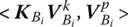 of a Lumped Mass Vibrating in Space
For a lumped mass with spatial vibrations
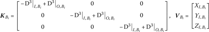
Let ![]() and
and ![]() . According to the continuous condition of a lumped mass
. According to the continuous condition of a lumped mass ![]() , so
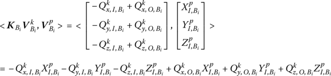
, so
where ![]() and
and ![]() denote the internal force of the system at the input and output ends, repectively, except for damping forces, which are correlated to the connected relations of a lumped mass in an MS.
denote the internal force of the system at the input and output ends, repectively, except for damping forces, which are correlated to the connected relations of a lumped mass in an MS.
For example, when a lumped mass Bi is connected to the lumped masses ![]() and
and ![]() by springs
by springs ![]() and
and ![]() in the input and output ends, respectively, we obtain
in the input and output ends, respectively, we obtain
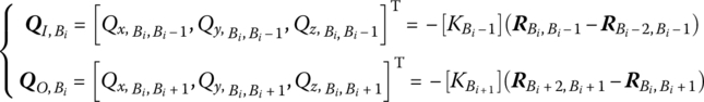
where

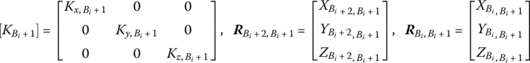
Substituting Equation (3.60) into Equation (3.59) yields
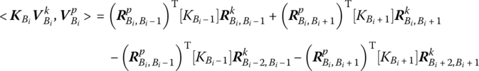
The superscripts k and p are symmetrical for the first two terms and unsymmetrical for the last two terms in Equation (3.61), therefore ![]() is unsymmetrical about
is unsymmetrical about ![]() in general. The signs of
in general. The signs of ![]() are opposite, corresponding to the input and output ends.
are opposite, corresponding to the input and output ends.
3.4.4.2  of a Rigid Body Vibrating in Space
For a rigid body vibrating in space with N input and L output ends


According to the geometry relations of a rigid body
therefore
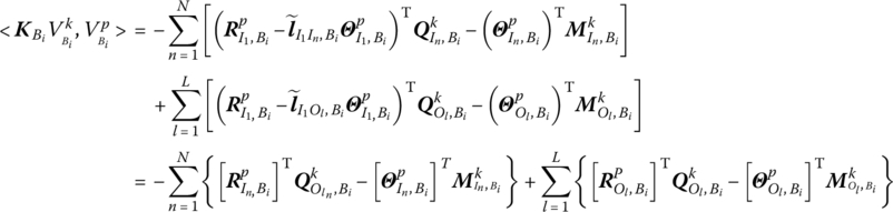
Equations (3.62) and (3.59) have the same form and physical meaning, but the signs of ![]() are opposite, corresponding to the input and output ends.
are opposite, corresponding to the input and output ends.
3.4.4.3  of a Beam Simultaneously Vibrating Transversely, Longitudinally and Torsionally
For a Euler–Bernoulli beam with uniform and constant sections simultaneously vibrating transversely, longitudinally and torsionally, we have
Thus
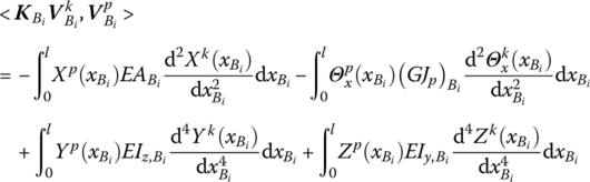
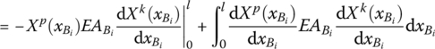
By the constitutive relations of a beam, we obtain
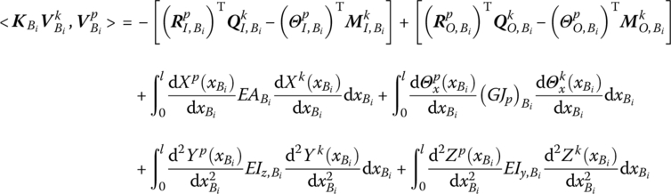
It can be seen from Equation (3.64) that the superscripts k and p are symmetrical for the four integral terms of the right‐hand side and unsymmetrical for terms related to the ends of the beam in general. These terms have the same physical meaning as Equation (3.59), and the signs of ![]() are opposite, corresponding to the input and output ends.
are opposite, corresponding to the input and output ends.
It can be seen from this discussion about the three kinds of typical body elements that ![]() is unsymmetrical about
is unsymmetrical about ![]() in general and the signs of
in general and the signs of ![]() are opposite, corresponding to the input and output ends. The stiffness parameter matrix
are opposite, corresponding to the input and output ends. The stiffness parameter matrix ![]() of a body element is an unsymmetrical matrix and the orthogonality of the augmented eigenvector V about augmented operator K should be proved from the point view of the system. We will prove V is symmetrical about K from the connection relations of the hinge elements and the boundary conditions of the system. For a rigid body, lumped mass or beam, the general unsymmetrical term about superscripts k and p of
of a body element is an unsymmetrical matrix and the orthogonality of the augmented eigenvector V about augmented operator K should be proved from the point view of the system. We will prove V is symmetrical about K from the connection relations of the hinge elements and the boundary conditions of the system. For a rigid body, lumped mass or beam, the general unsymmetrical term about superscripts k and p of ![]() is
is
where the subscript P denotes the connection point.
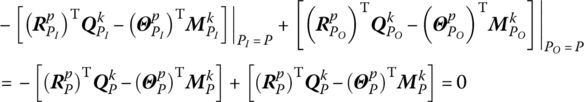
These terms are all the products of internal force and displacement of the connection point or internal moment and angular displacement, and the signs are always negative for the input end and positive for the output end of the body element:
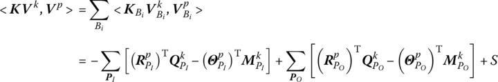
where PI and PO are the set constituted by the input and output ends, respectively, of all body elements in the system, PI and PO are the elements corresponding to PI and PO, and S is the summation of symmetrical terms about k and p in ![]() .
.
For an MRFS composed of rigid bodies, lumped masses and beams connected by various hinges, the connection points are the input end (or output end) of one element and the output end (or input end) of another, except for the boundary ends. Hence, only the parameters of the input and output ends of the body elements are involved for the first two terms of the right‐hand side of Equation (3.66), which can be classified into the following six cases in which k and p are symmetrical.
- The input end of a body element is the input boundary of the system.
Such a point is denoted by P in the first term of the right‐hand side of Equation (3.64),
 , therefore for homogeneous boundary conditions there are always
Obviously, k and p are symmetrical in Equation (3.67).
- The output end of the body element is the output boundary of the system.
Such a point is denoted by P in the second term on the right‐hand side of Equation (3.66),
 , therefore for homogeneous boundary conditions there are always
Obviously, k and p are symmetrical in Equation (3.68).
- The input end of the body element is the output end of another body element.
This point is denoted by P in the first term on the right‐hand side of Equation (3.66),
 . This point is also denoted by P in the second term on the right‐hand side of Equation (3.66),
 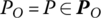 :
:Obviously, k and p are symmetrical in Equation (3.69).
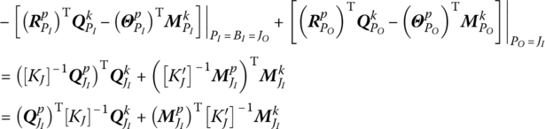
- The input end of the body element is the output end of the hinge element.
This point is denoted by BI in the first term of the right‐hand side of Equation (3.66) and the input end of the body element. The output end of the hinge element is denoted by JO. BI and JO are the same points, namely
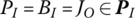 . Suppose that the input end of the hinge element is JI and this must be the output end of the other body element. This point is included in the second term of the right‐hand side of Equation (3.66), namely,
  . Since the internal forces (moments) are always equal for the input and output ends of the hinge element, namely(3.70)
then
(3.71)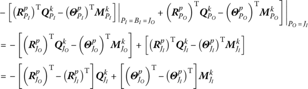
For a linear system, the internal force and the internal moment are linearly correlated to the deformations of the hinge in the following forms
(3.72)
where [KJ] and
 denote the stiffness coefficient matrices of the hinge element J. They are the real constant symmetrical matrix
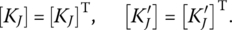
Substituting Equation (3.58) into Equation (3.57), we obtain
Obviously, k and p are symmetrical in Equation (3.73).
- The output end of a body element is the input end of another body element.
The proof of this is the same as (3), and k and p are symmetrical.
- The output end of a body element is the input end of the hinge element.
The proof of this is similar to (4), where k and p are symmetrical, and we will not discuss this in detail.
In summary, the superscripts k and p in Equation (3.66) are symmetrical for a real system, therefore the augmented eigenvector is symmetrical about the augmented operator K and the second equation in Equation (3.52) is satisfied automatically.
3.5 Examples of the Orthogonality of Augmented Eigenvectors
Augmented eigenvector orthogonality covers the orthogonality of the eigenfunctions of a continuous system and the eigenvectors of a discrete system, thus both of them can be regarded as special cases of the orthogonality for augmented eigenvectors of MRFS.
3.6 Transient Response of a Multibody System
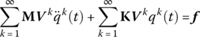
The body dynamics equation of an undamped MRFS is
The physical coordinate of the dynamics response may be expanded using augmented eigenvectors Vk as
Substituting Equation (3.91) into Equation (3.90) yields
Take the inner product for both sides of Equation (3.92) using augmented eigenvectors ![]() and the orthogonality of the augmented eigenvectors:
and the orthogonality of the augmented eigenvectors:
The generalized coordinate equations of the system can be obtained:
Assume that the initial conditions of the MRFS are
This yields

We obtain

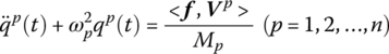
Equation (3.94) is the forced vibration equation of the system in generalized principal coordinates. The eigenfrequencies ![]() and the corresponding augmented eigenvectors Vp can be acquired using the method illustrated above. The generalized coordinates
and the corresponding augmented eigenvectors Vp can be acquired using the method illustrated above. The generalized coordinates ![]() can be obtained by integrating Equation (3.94) with respect to time one by one. The dynamics response of the system can be determined by Equation (3.91). Note that
can be obtained by integrating Equation (3.94) with respect to time one by one. The dynamics response of the system can be determined by Equation (3.91). Note that ![]() is a single‐valued function depending only on time t, and the solutions of generalized coordinates are found out as
is a single‐valued function depending only on time t, and the solutions of generalized coordinates are found out as
therefore the dynamics response of the system is
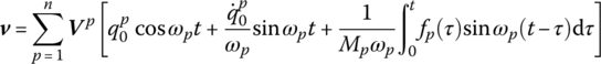
Figure 3.2 Time history of the displacement of the free end of beam 3.
Figure 3.3 A planar vibration system composed of a spring, lumped mass and beam.
Table 3.1 Generalized speed corresponding to partial velocity
| r | ur | Partial velocity | ||
| VC | VP | VQ | ||
| 1 | u1 | e | e | e |
| 1 + j |
|
0 |
|
0 |
Table 3.2 Computational results of eigenfrequency (rad/s)
| Mode | 1 | 2 | 3 | 4 | 5 | 6 | 7 | 8 |
| Analytical method | 0.8136 | 4.0820 | 6.7085 | 15.2696 | 29.0900 | 47.5685 | 70.6657 | 98.3774 |
| Kane’s method | 0.8223 | 5.1534 | – | 14.4298 | 28.2766 | 46.7432 | 69.8263 | 97.5259 |
| MSTMM | 0.8136 | 4.0820 | 6.7085 | 15.2696 | 29.0900 | 47.5685 | 70.6657 | 98.3774 |
Figure 3.4 The time history of displacement of the free end of the beam.
Figure 3.5 The time history of displacement at the free end of beam for Ki = 10000 N/m.
3.7 Steady‐state Response of a Damped Multibody System
3.7.1 Treatment of the Damping Forces in a Multibody System
The body dynamics equation of a viscous‐damped MRFS is
where C is the damping augmented operator of the system.
Substituting ![]() into Equation (3.135) yields
into Equation (3.135) yields
Taking the inner product for ![]() on both sides of Equation (3.136) yields
on both sides of Equation (3.136) yields

General speaking, the augmented eigenvector is not orthogonal with respect to the damping augmented operator C, namely for ![]() the equation
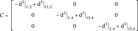
the equation ![]() does not always hold. Thus, the coordinates in Equation (3.137) are still coupled. Taking the system shown in Figure 3.6 as an example, it is easy to write the damping augmented operator of this system:
does not always hold. Thus, the coordinates in Equation (3.137) are still coupled. Taking the system shown in Figure 3.6 as an example, it is easy to write the damping augmented operator of this system:

Figure 3.6 A damped system with three degrees of freedom.
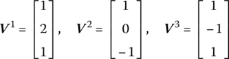
The augmented eigenvectors ![]() of the system are
of the system are
Noting that ![]() , then
, then

Obviously, [Ckp] is not a diagonal matrix, namely, for ![]() ,
, ![]() .
.
The vibration analysis is extremely complex since the coordinates are coupled in Equation (3.137). To use the modal analysis used for the undamped system, the following approximate methods for engineering are applied.
3.7.1.1 Neglecting all the Nondiagonal Elements of Matrix [Ckp]
The procedure in practice is to let
The matrix [Ckp] become a diagonal matrix

where Cp is the damping coefficient of the pth‐order principal mode, which is known as the pth‐order mode damping or modal damping.
Hence, Equation (3.137) is decoupled and the pth equation becomes
Both sides of Equation (3.143) are divided by Mp, then let
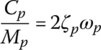
Then Equation (3.143) becomes
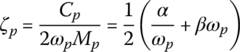
where ζp is the pth‐order mode damping ratio or modal damping ratio.
A fairly good approximate solution can usually be obtained with this treatment for general engineering problems.
3.7.1.2 Assumption of Proportional Damping
In this method, the damping parameter matrix is assumed to be proportional to the mass and stiffness parameter matrices
where α and β are constants.
By using the orthogonality of augmented eigenvectors, we obtain
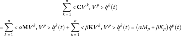
Obviously Equation (3.147) is decoupled and thus
By rewriting Equation (3.144), we obtain
The first and second terms on the right‐hand side of Equation (3.149) are inversely proportional and proportional, respectively, to the eigenfrequency ωp. Hence, α and β affect mainly low and high frequencies, respectively.
3.7.1.3 Determine each Mode Damping Ratio by Experiment
Until now the mechanisms of damping have not been clear, and it has been difficult to measure or compute accurately the practical damping matrix. The mode damping ratio is usually measured directly by experiment when ![]() in practice and then each parameter in Equation (3.145) is obtained.
in practice and then each parameter in Equation (3.145) is obtained.
3.7.1.4 Take Damping as an External Force
If the external force vector f acting on MRFS relates to the displacement, velocity and other parameters of the system, the inner product ![]() will contain the generalized coordinates qp(t) and the terms corresponding to dampings in Equation (3.137) may be treated as external forces, namely
will contain the generalized coordinates qp(t) and the terms corresponding to dampings in Equation (3.137) may be treated as external forces, namely

Then, Equation (3.137) becomes

In fact, Equation (3.151) has not been decoupled. If the value fp in any time is instead given by its value the previous time, the computation and programming may be simplified greatly. It is impossible to decouple completely the dynamics equations for many practical engineering applications because of their time variance and nonlinearity, therefore this approach is very useful.
3.7.1.5 Damping Linear Operator
For convenience, the damping linear operator can be defined as follows for complex MRFS:

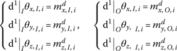
where i is the sequence number of the body element, I and O denote the input and output ends, and, ![]() and
and ![]() and,
and, ![]() and
and ![]() denote damping forces and damping moments.
denote damping forces and damping moments.
The combination of the damping linear operator d3 and the displacement of a point of a body element results in the damping force acting on this point, while the combination of the operator d1 and an angular displacement of a point of a body element leads to the damping moment acting on this point. For example, using the linear operator d3, the damping force acting on the body element of sequence number i in the system shown in Figure 3.5 can be written as
The damping augmented operator of the system is
3.7.2 Steady‐state Response of a Damped Multibody System
3.7.2.1 Approximate Solution of the Dynamics Responses of a Multibody System
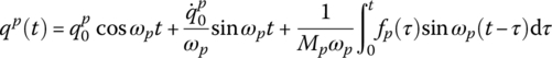
According to the approximate treatment methods for damping discussed in Section 3.7.1, the solution of differential Equation (3.145) in term of generalized coordinates is obtained as follows

where
ωd, p is the pth‐order damped eigenfrequency.
Substituting qp(t) into
gives the dynamics response of the system to arbitrary excitation.
3.7.2.2 The General Solution of Dynamics Responses of MRFS
The general steps for solving the dynamic response of a damped MRFS to arbitrary excitation using the mode superposition method are as follows.
- Compute the vibration characteristic of the undamped system.
- Write the body dynamics equations of the system and construct the augmented eigenvectors of the undamped system.
- Decouple the body dynamics equations of the system using the orthogonality of the augmented eigenvectors and transform the partial differential equations to ordinary differential equations, dealing with the damping according to the methods described in Section 3.7.1.
- Compute the initial conditions and excitation force under the generalized coordinates.
- Compute the generalized coordinates of the system.
- Compute the dynamics responses in physical coordinates using generalized coordinates and augmented eigenvectors.
Figure 3.7 A damped system vibrating in a plane.
Figure 3.8 The computational result of the dynamics response of a damped plane vibration system: (a) time history of displacement of lumped mass 2, (b) time history of displacement of the free end of beam 3, (c) time history of displacement of lamped mass 2 and (d) time history of displacement of the free end of beam 3.
3.8 Steady‐state Response of a Multibody System
3.8.1 Steady‐state Response of a Multibody System to Harmonic Excitation
3.8.1.1 Steady‐state Response of a Single DOF System to Harmonic Excitation
The dynamics equation of a damped system with a single DOF under a harmonic force ![]() is
is
Note that if ![]() , then
, then
where F and α are the amplitude and phase of the exciting force F(t), respectively. ![]() .
.
F(t) can be written as
where ![]() .
.
Then Equation (3.69) can be written as
The steady‐state solution of Equation (3.172) is ![]() , where
, where ![]() is the complex amplitude of forced vibration. Substituting this into Equation (3.172) yields
is the complex amplitude of forced vibration. Substituting this into Equation (3.172) yields
where
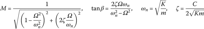
M is the magnification factor of the dynamic vibration amplitude and β is the phase‐lag angle of response x relative exciting force F(t).
The steady‐state response of the system is
3.8.1.2 Steady‐state Response of a MRFS to Harmonic Excitation
The body dynamics equation of a damped MRFS under an external force ![]() is
is
Note that f(t) cannot be written in the form of ![]() . However, using the orthogonality of the augmented eigenvectors and the simplification treatment for damping, we can obtain
. However, using the orthogonality of the augmented eigenvectors and the simplification treatment for damping, we can obtain
Note that if ![]() , then
, then
Comparing Equation (3.178) with Equation (3.169), and using the results of section 3.8.1.1, yields

where

Mp is the magnification factor of the vibration amplitude of pth‐order and βp is the phase‐lag angle of principal coordinate qp(t) of pth‐order relative to exciting force Fp(t).
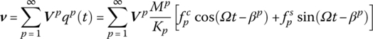
The steady‐state response of the system is then
3.8.1.3 Solve the Steady‐state Response of an MRFS under Harmonic Excitation Using the Extended MSTMM
The solution of the steady‐state response of an MRFS under harmonic excitation using the extended MSTMM has been discussed in Chapter 2. The computational time needed for this method is less than that for the method used in section 3.8.1.2. Only the calculation of the extended transfer matrices should be carried out, and the vibration characteristic of the system does not need to be solved. The approximate treatment for damping is necessary and only the approximate solution can be obtained if using the method used in section 3.8.1.2. The extended MSTMM results in an exact solution of the system.
3.8.2 Steady‐state Response of a Multibody System to Periodic Excitation
The body dynamics equation of a damped MRFS is
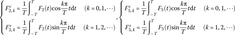
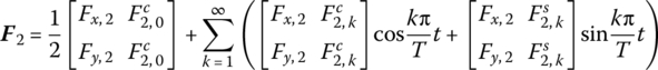
If the external force f(t) is a function of period 2 T, it can be expanded using Fourier series as follows
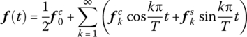
where
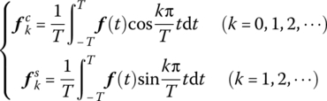
![]() are constant column matrices.
are constant column matrices.
With the method used in part (3) of section 3.8.1 the steady‐state responses ![]() can be obtained by solving the following equations
can be obtained by solving the following equations
The steady‐state response of the system ![]() can be obtained by superposition of
can be obtained by superposition of ![]() .
.
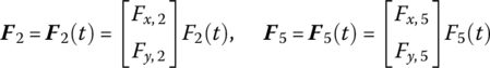
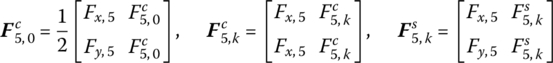
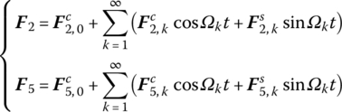
It should be pointed out that this process is only the mathematical explanation to solve steady‐state response, and the practical method of solving ![]() is still by extended transfer matrix method. For example in part (3) in section 3.8.1, the external force F2 appears in the extended transfer matrix Û2 in the form of
is still by extended transfer matrix method. For example in part (3) in section 3.8.1, the external force F2 appears in the extended transfer matrix Û2 in the form of ![]() , and the external force F5 appears in the extended transfer matrix Û5 in the form of
, and the external force F5 appears in the extended transfer matrix Û5 in the form of ![]() . Equation (3.182) is solved rather than directly using Equation (3.183). We still use the above‐mentioned MRFS to explain the solving process.
. Equation (3.182) is solved rather than directly using Equation (3.183). We still use the above‐mentioned MRFS to explain the solving process.
In the above example, assume that
where

![]() and
and ![]() are constant real numbers.
are constant real numbers.
Substituting Equation (3.187) into Equation (3.186) yields

Note that if

then
Using the same method and steps as in part (3) of section 3.8.1, the steady‐state response v0 of the system under the static load ![]() and
and ![]() is solved first. Then the steady‐state responses
is solved first. Then the steady‐state responses ![]() under the harmonic forces F2, k and F5, k with frequency Ωk are computed one by one, and finally the steady‐state response of the system excited by an external force with a period of 2 T is obtained as
under the harmonic forces F2, k and F5, k with frequency Ωk are computed one by one, and finally the steady‐state response of the system excited by an external force with a period of 2 T is obtained as
Figure 3.9 Steady‐state response of the free end of the beam.
3.9 Static Response of a Multibody System
Static force can be treated as a periodic force of frequency Ω = 0. The steady‐state response of MRFS to a static force can be solved as a periodic force. The effect of the inertia and damping of such a system need not to be considered. This greatly reduces the order of matrices and the computational scale.

Figure 3.10 Mechanics model of a barrel assembly for static deformation.
Figure 3.11 Computational results of the static response of the gun tube: (a) the static deflection of the gun tube, (b) the rotation angle of the gun tube, (c) the moment of the gun tube and (d) the shear force of the gun tube.