15
Transfer Matrix Library for Multibody Systems
15.1 Introdution
Applying transfer matrix method for multibody systems (MSTMM) to solve the eigenvalue problem of linear time‐invariant multibody systems, steady‐state response and the dynamics problem of general multibody systems requires the transfer matrices of elements to be gathered into the overall transfer matrix of the system. From the boundary conditions of the system, we can easily compute the dynamics of the system by solving the overall transfer equation and the transfer equation of each element. The transfer matrix of each element has an important feature, that is, the element has the same transfer matrix even in a different system if it has the same connection relationship and motion mode. This feature makes the solution process of multibody system dynamics very simple and convenient. Once the transfer matrix of a certain element has been derived, it can be used for the same kind of elements in different multibody systems.
The transfer matrices of various elements [279–452] are listed in this chapter so readers can check them when they are needed. If the transfer matrix of a new element is not found in this chapter, readers can derive the corresponding transfer matrix using the proposed methods in Chapters 5, 6, 7, 8 and 10, and add it to the transfer matrix library. The transfer matrix library can be used to solve the dynamics problems of various complex multibody systems, including chain multibody systems, branch multibody systems, closed‐loop multibody systems, network multibody systems and controlled multibody systems, for example the eigenvalue problem of linear multibody systems, the steady‐state response of linear multibody systems, the steady‐state response of nonlinear multibody systems, the dynamics of multi‐rigid‐body systems (MRSs), the dynamics of multi‐rigid‐flexible‐body systems (MRFSs) and the dynamics of controlled systems. The library of transfer matrices for multibody systems provides an important tool for setting up dynamic simulation software with powerful functions and high computational speed. This is an important research branch in this field. Readers and experts in other fields are welcome to cooperate in this area by supplying the transfer matrices of new elements in research and engineering which are not listed in this library. The authors will continue to provide the transfer matrices of new elements, and add bricks and tiles to the development of the transfer matrix library for multibody systems, the MSTMM and MBD.
15.2 Springs
Different kinds of springs are shown in Figure 15.1.

Figure 15.1 Springs for longitudinal vibrations: (a) one‐dimensional, (b) two‐dimensional and (c) three‐dimensional.
15.2.1 One‐dimensional Longitudinal Vibration
The state vector is
The transfer matrix is
where Kx is the stiffness of the spring.
15.2.2 Longitudinal Vibration in Plane
The state vector is
The transfer matrix is
where Kx and Ky are the stiffnesses of the springs in the x and y directions, respectively.
15.2.3 Longitudinal Vibration in Space
The state vector is
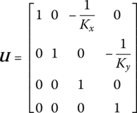
The transfer matrix is
where Kx, Ky and Kz are the stiffnesses of the springs in the x, y and z directions, respectively.
15.3 Rotary Springs
Different kinds of rotary springs are shown in Figure 15.2.
Figure 15.2 Rotary springs of torsion vibration: (a) one‐dimensional, (b) two‐dimensional and (c) three‐dimensional.
15.3.1 One‐dimensional Torsional Vibration
The state vector is
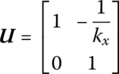
The transfer matrix is

where ![]() is the torsional stiffness of the rotary spring.
is the torsional stiffness of the rotary spring.
15.3.2 Torsional Vibration in Plane
The state vector is
The transfer matrix is
where ![]() are the torsional stiffnesses of the rotary springs about the x and z directions, respectively.
are the torsional stiffnesses of the rotary springs about the x and z directions, respectively.
15.3.3 Torsional Vibration in Space
The state vector is
The transfer matrix is
where ![]() are the torsional stiffnesses of the rotary springs about the x, y and z axes, respectively.
are the torsional stiffnesses of the rotary springs about the x, y and z axes, respectively.
15.4 Elastic Hinges
Different of elastic hinges are shown in Figure 15.3.

Figure 15.3 Elastic hinges: (a) planar elastic hinge and (b) spacial elastic hinge.
15.4.1 The Planar Elastic Hinge
The state vector is
The transfer matrix is
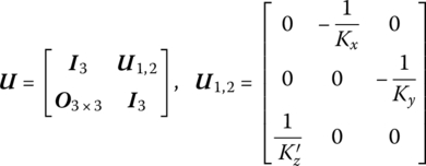
where Kx and Ky are the stiffness of the springs in the x and y directions, respectively, and ![]() is the torsional stiffness of the rotary spring in the z direction.
is the torsional stiffness of the rotary spring in the z direction.
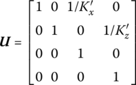
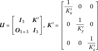
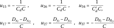
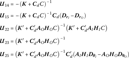
15.4.2 The Spatial Elastic Hinge
The state vector is
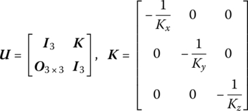
The transfer matrix is
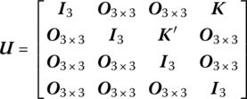
where
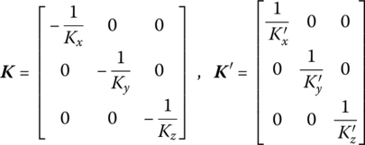
where Kx, Ky and Kz are the stiffnesses of the springs in the x, y and z directions, respectively, and ![]() are the torsional stiffness of the rotary springs about the x, y and z axes, respectively.
are the torsional stiffness of the rotary springs about the x, y and z axes, respectively.
15.5 Lumped Mass Vibrating in a Longitudinal Direction
15.5.1 Lumped Mass with Longitudinal Vibration
The state vector is
The transfer matrix is
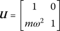
where m is the mass of the lumped mass and ω is the eigenfrequency.
15.5.2 Lumped Mass with Longitudinal Vibration in a Plane
The state vector is
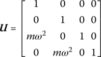
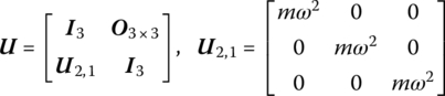
The transfer matrix is
15.5.3 Lumped Mass with Longitudinal Vibration in Space
The state vector is
The transfer matrix is
15.6 Vibration of Rigid Bodies
15.6.1 Planar Vibration of a Rigid Body with One Input End and One Output End
The state vector is
The transfer matrix is
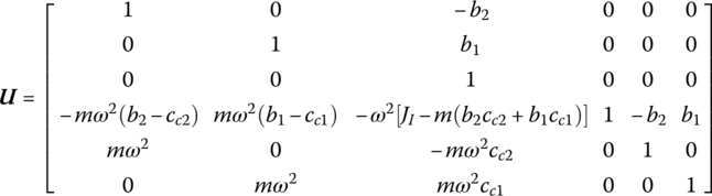
where ω is the eigenfrequency, m is the mass of the rigid body and JI is the moment of inertia with respect to point I. (b1, b2) are the position coordinates of the output end O and (cc1, cc2) are the position coordinates of the mass center C.
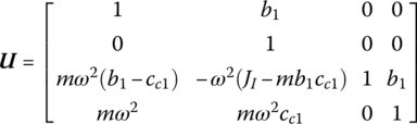
If only the transverse displacement and torsional vibration of the rigid body are considered, the longitudinal displacement can be neglected and the state vector is defined as
The transfer matrix is
15.6.2 Spatial Vibration of a Rigid Body with One Input End and One Output End
The state vector is
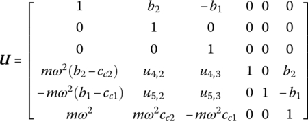
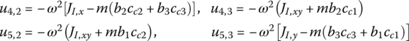
The transfer matrix is
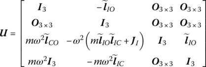
where
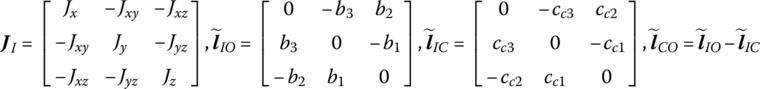
which is decomposed in a body‐fixed coordinate system with origin the input end I, ![]() is the inertia matrix with respect to point I, (b1, b2, b3) are the position coordinates of the output end O and (cc1, cc2, cc3) are the position coordinates of the mass center C.
is the inertia matrix with respect to point I, (b1, b2, b3) are the position coordinates of the output end O and (cc1, cc2, cc3) are the position coordinates of the mass center C.
The state vector is defined as
The corresponding transfer matrix is
where
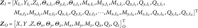
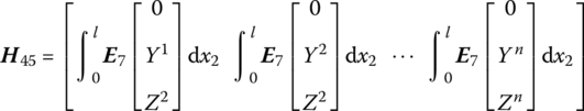
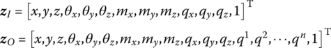
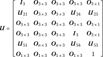
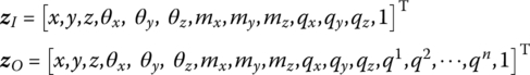
15.6.3 Spatial Vibration of a Rigid Body with N Input Ends and L Output Ends
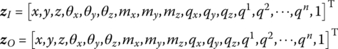
The state vectors are
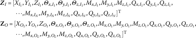
The transfer equation is
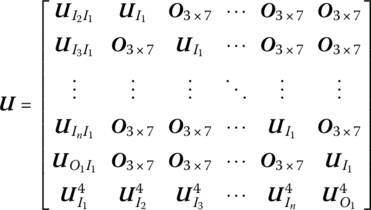
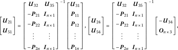
The transfer matrices are

The related structural parameters are described in the body‐fixed coordinate system whose origin is the first input end I1.
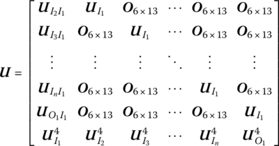
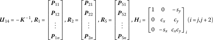
15.6.4 Spatial Vibration of a Rigid Body with N Input Ends and One Output End
The state vectors are
The transfer equation is
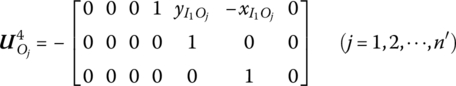
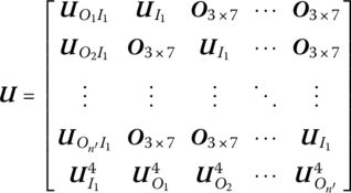
The transfer matrix is
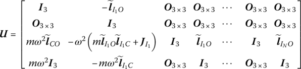
where ![]() is the nth input end. The related structural parameters are described in the body‐fixed coordinate system whose origin is the first input end I1 and
is the nth input end. The related structural parameters are described in the body‐fixed coordinate system whose origin is the first input end I1 and ![]() is the inertia matrix with respect to I1.
is the inertia matrix with respect to I1.
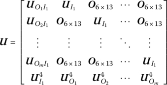
15.6.5 Spatial Vibration of a Rigid Body with One Input End and L Output Ends
The state vectors are
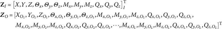
The transfer matrix is
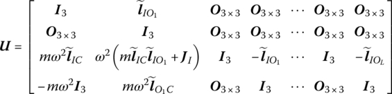
where ![]() is the lth output end. The related structural parameters are described in the body‐fixed coordinate system whose origin is located at input end I. It should be noted that the transfer equation in this case is
is the lth output end. The related structural parameters are described in the body‐fixed coordinate system whose origin is located at input end I. It should be noted that the transfer equation in this case is ![]() .
.
15.7 Beam with Transverse Vibration
The state vector is
15.7.1 Euler–Bernoulli Beam with Transverse Vibration
The transfer matrix is
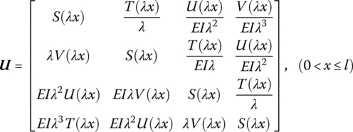
where S, V, U and T are the Кpылoв functions:
where l is the length of the beam, ![]() , EI is the bending stiffness of the beam and
, EI is the bending stiffness of the beam and ![]() is the line mass density of the beam.
is the line mass density of the beam.
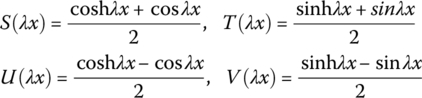
15.7.2 Timoshenko Beam with Transverse Vibration
The transfer matrix is
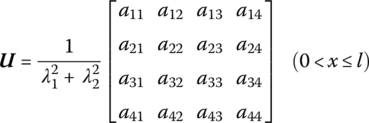
where
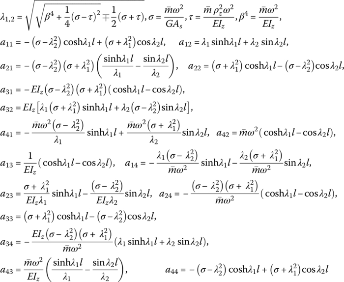
where l is the length of the beam, EI is the bending stiffness of the beam and ![]() is the line mass density of the beam. A is the cross‐section area, Iz is the moment of inertia of the cross‐section with respect to the neutral line and ρz is the gyration radius of the cross‐section with respect to the neutral line.
is the line mass density of the beam. A is the cross‐section area, Iz is the moment of inertia of the cross‐section with respect to the neutral line and ρz is the gyration radius of the cross‐section with respect to the neutral line. ![]() is the shear stiffness and κs is the shape factor determined by the shape of the cross‐section.
is the shear stiffness and κs is the shape factor determined by the shape of the cross‐section.
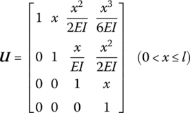
15.7.3 Massless Euler–Bernoulli Beam with Transverse Vibration
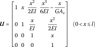
The transfer matrix is
Considering the influence of shear deformation, the transfer matrix of the massless Euler–Bernoulli beam with transverse vibration is
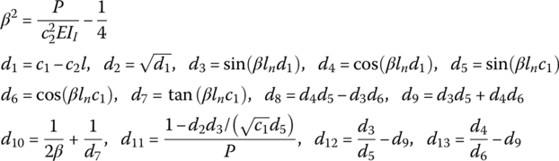
15.7.4 Massless Euler–Bernoulli Beam with Axial Load and Shear Deformation
The transfer matrix is
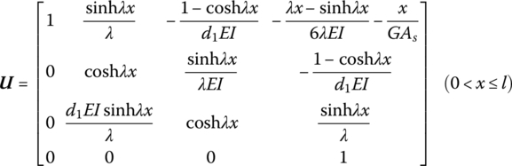
where for the axial compressive force P, ![]() and
and ![]() . For the axial tensile force P,
. For the axial tensile force P, ![]() and
and ![]() .
.
15.7.5 Massless Euler–Bernoulli Beam with Elastic Foundation
The transfer matrix is
where
where z ![]() , k* is the Winckler (elastic) modulus of the foundation and
, k* is the Winckler (elastic) modulus of the foundation and ![]() .
.
15.7.6 Massless Transverse Vibrational Euler–Bernoulli Beam with Elastic Foundation
The massless transverse vibrational Euler–Bernoulli beam with elastic foundation is shown in Figure 15.4.
Figure 15.4 A transverse vibrational rigid beam with elastic foundation.
The transfer matrix is
where K* is the Winckler (elastic) modulus of the foundation, K′* is the rotational (elastic) modulus of the foundation and r is the gyration radius of the cross‐section about the z axis.
15.7.7 Flexible Point Support
Different kinds of flexible point supports are shown in Figure 15.5.
Figure 15.5 Elastic point support: (a) spring, (b) rotary spring and (c) elastic hinge.
The transfer matrices of the flexible points supported by spring, rotary spring and elastic hinges are
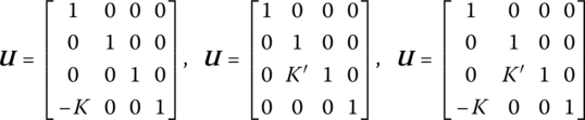
where K is the translational stiffness of the support and K′ is the torsional stiffness.
If there is a lumped mass at the support point, the rotary inertia of the lumped mass is considered. Then the corresponding transfer matrix is
where m is the mass of the lumped mass and J is the moment of inertia of the lumped mass.
15.7.8 Nonuniform Cross‐section Euler–Bernoulli Beam with Axial Compressive Force
A nonuniform cross‐section Euler–Bernoulli beam with axial compressive force is shown in Figure 15.6.
Figure 15.6 Nonuniform cross‐section Euler–Bernoulli beam with axial compressive force. (a) The output end is thinner than the input end. (b) The output end is thicker than the input end.
The transfer matrix is
where
15.8 Shaft with Torsional Vibration
The state vector is
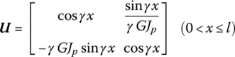
15.8.1 Torsional Vibration of an Elastic Shaft with Uniform Cross‐section
The transfer matrix is

where l is the length of the shaft, ![]() and ρ is the mass density of the shaft. Jp is the polar inertia of the cross‐section of the shaft and GJp is the torsional stiffness of the shaft.
and ρ is the mass density of the shaft. Jp is the polar inertia of the cross‐section of the shaft and GJp is the torsional stiffness of the shaft.
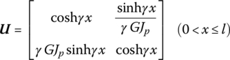
15.8.2 Torsional Vibration of a Massless Elastic Shaft with Uniform Cross‐section
The transfer matrix is
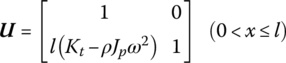
15.8.3 Massless Torsional Vibrational Elastic Shaft with Elastic Foundation and Uniform Cross‐section
The transfer matrix is
where ![]() and Kt is the elastic modulus of the foundation.
and Kt is the elastic modulus of the foundation.
15.8.4 Torsional Vibration of a Rigid Shaft with Elastic Foundation
The transfer matrix is
15.8.5 Torsional Vibration of an Elastic Shaft with Elastic Foundation and Uniform Cross‐section
The transfer matrix is
where 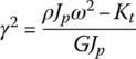 . If
. If ![]() ,
, 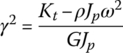 and Equation (15.32) are used.
15.8.6 Flexible Point Support of a Lumped Mass on a Torsional Vibrational Shaft
The transfer matrix is
where ![]() is the torsional stiffness of the flexible point support and J is the moment of inertia of the lumped mass.
is the torsional stiffness of the flexible point support and J is the moment of inertia of the lumped mass.
15.9 Rod with Longitudinal Vibration
The state vector is
15.9.1 Longitudinal Vibration of an Elastic Rod with Uniform Cross‐section
The transfer matrix is
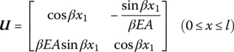
where l is the length of the rod, EA is the tensile stiffness,  and
and ![]() is the mass per unit length.
is the mass per unit length.
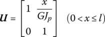
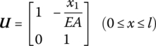
15.9.2 Longitudinal Vibration of a Massless Elastic Rod with Uniform Cross‐section
The transfer matrix is
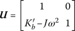
15.9.3 Flexible Point Support of a Lumped Mass on a Translational Vibrational Rod
The transfer matrix is
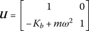
where Kb is the elastic coefficient of the flexible point support and m is the mass of the lumped mass.
15.10 Euler–Bernoulli Beam
15.10.1 Euler–Bernoulli Beam Vibrating Longitudinally in the x Direction and Transversely in the y Direction
The state vector is
The transfer matrix is

where 0 ≤ x1 ≤ l, ![]() and
and ![]() .
.
15.10.2 Euler–Bernoulli Beam Vibrating Torsionally about the x Axis and Transversely in the z Direction
The state vector is
The transfer matrix is
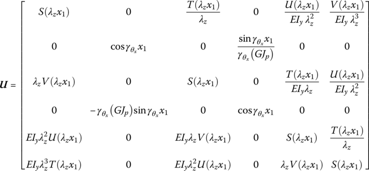
where 0 ≤ x1 ≤ l, ![]() and
and ![]() .
.
15.10.3 Euler–Bernoulli Beam Vibrating Torsionally about the x Axis, Longitudinally in the x Direction and Transversely in the y and z Directions
The state vector is
The transfer matrix is
where

If the longitudinal motion in the x direction and the rotation about x axis are regarded as rigid motion, then
15.11 Rectangular Plate
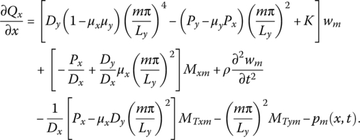
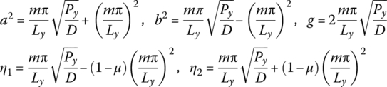
15.11.1 Dynamic Equations of an Anisotropic Rectangle Plate
For an orthogonal anisotropic rectangle plate, as shown in Figure 15.7, the basic equations of the bending motion [38] are
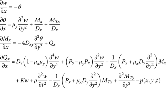
where
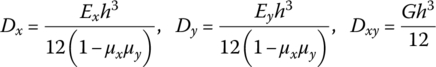

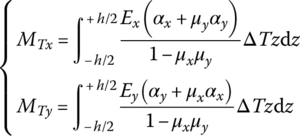
Px and Py are the planar pressure, w is the transverse deflection, Dx, Dy and Dxy are the flexural stiffness, and μx and μy are the Poisson’s ratios with respect to the x and y axes, respectively. ρ is the mass density, K is the elastic modulus of the foundation and p is the distributed transversely loading intensity. Ex and Ey are the material elastic moduli with respect to the x and y axes, respectively. G is the shear elastic modulus of the material, h is the thickness of the plate and ΔT is the temperature variation. αx and αy are the heat expansion coefficients with respect to the x and y axes, respectively. Mx and My are the bending moments, Myx and Mxy are torsional moments, and Qx and Qy are the shear forces.
Figure 15.7 Positive deflection, internal bending moment and shearing force.
Equation (15.43) can be written as

where ![]() .
.
If the pressures Px and Py are replaced by ![]() and
and ![]() , then Equation (15.43) and Equation (15.47) are valid for the case with a tensile force.
, then Equation (15.43) and Equation (15.47) are valid for the case with a tensile force.
If the proposed plate is simply supported on both sides of ![]() and
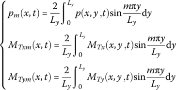
and ![]() , the variables w, θ, Mx and Qx can be expanded in Fourier series. Deleting the variable y in Equation (15.46) yields
, the variables w, θ, Mx and Qx can be expanded in Fourier series. Deleting the variable y in Equation (15.46) yields

The mechanical load and heat load can be expanded as follows

therefore
Substituting Equations (15.49) and (15.50) into Equations (15.43) and (15.52) gives
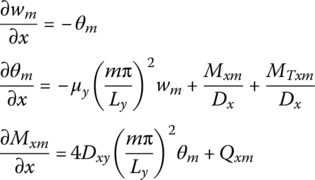
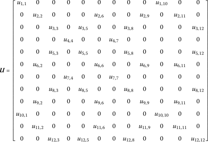
The state vector is defined as
The corresponding transfer matrix can be obtained as follows.
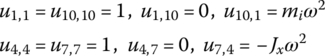
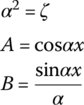
15.11.2 Massless Isotropic Rectangle Plate
The transfer matrix is
where ![]() ,
, ![]() and
and ![]() , and
, and
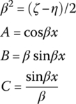
15.11.3 Isotropic Rectangle Plate with Axial Force
The transfer matrix is

where ![]() ,
, ![]() ,
, ![]() and
and ![]() .
.
For the plate with free vibration
For the plate under the planar pressure ![]() and
and ![]() , we get
, we get
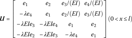
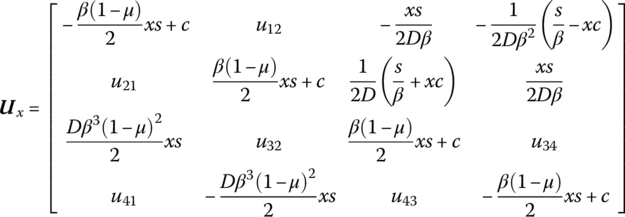
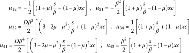
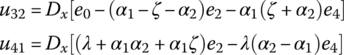
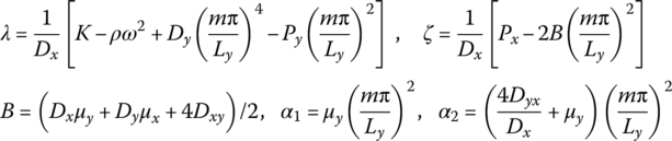
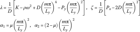
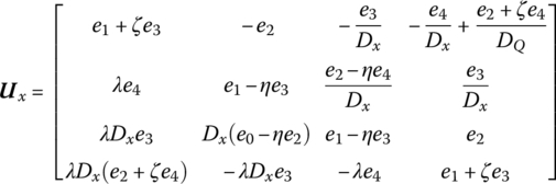
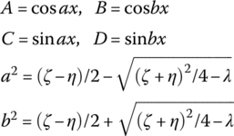
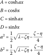
15.11.4 General Rectangle Plate
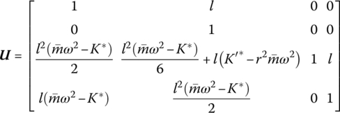
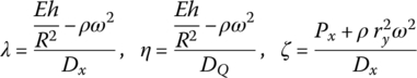
The transfer matrix is
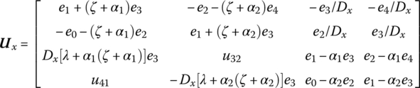
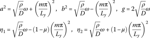
where
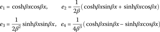
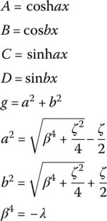
Px and Py are the pressures, if the planar force is tensile, Px and Py should be replaced by ![]() , and e0, e1, e2, e3 and e4 are shown in Table 15.1.
, and e0, e1, e2, e3 and e4 are shown in Table 15.1.
Table 15.1 The expression of e0, e1, e2, e3 and e4
| e0 |
|
|
|
|
|
|
| e1 |
|
A |
|
|
|
|
| e2 |
|
B |
|
|
|
|
| e3 |
|
|
|
|
|
|
|
|
||||||
 |
|
|
 |
|
 |
|
|
|
||||||
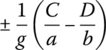
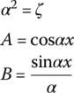
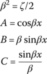
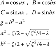
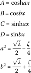
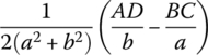
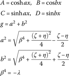
A, B, C, D, g, a and b in Table 15.1 are shown in Table 15.2.
Table 15.2 The expression of A, B, C, D, g, a and b
 |
 |
 |
 |
 |
 |
 |
 |
||
For the orthogonal anisotropic plate
For the isotropic plate
15.12 Disk
15.12.1 Dynamic Equations of a Disk
As shown in Figure 15.8, the disk acts on a symmetrical load. Its basic dynamic equations of flexural motion are
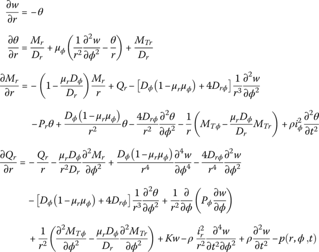
where
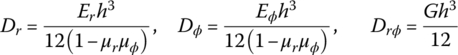
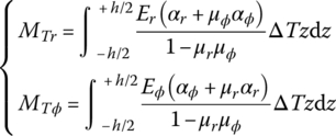
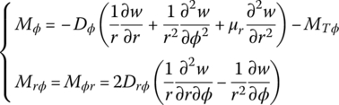

Figure 15.8 Positive deflection, slope, bending moment and shearing force.
Pr and Pϕ are the planar pressures, w is the transverse deflection and Dr, Dϕ and Drϕ are the bending stiffnesses. μr and μϕ are the Poisson’s ratios with respect to the r and ϕ directions, respectively. ρ is the mass density, and ir and iϕ are the rotational gyration radius around the axial and tangent directions, respectively. K is the elastic modulus of the foundation, p is the distributed transverse loading intensity, and Er and Eϕ are the material elastic modulus with respect to the direction of r and ϕ. G is the material shear elastic modulus, h is the thickness of the plate and ΔT is the temperature variation. αr and αϕ are the heat expansion coefficients with respect to the direction of r and ϕ. Mr and Mϕ are the bending moments, and Mrϕ and Mϕr are the torsional moments.
If an isotropic disk only vibrates transversely, Equation (15.56) is usually written as the fourth‐order basic equation:

where

If the pressures Px and Py are replaced by ![]() , then Equation (15.56) or Equation (15.60) is also valid for tensile forces.
, then Equation (15.56) or Equation (15.60) is also valid for tensile forces.
The variables w, θ, Mr and Qr can be expanded in Fourier series as follows
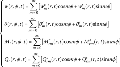
For a symmetrical motion (![]() ), Equation (15.61) can be further simplified:
), Equation (15.61) can be further simplified:
The mechanical load and heat load are expanded as follows:
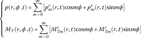
Substituting Equations (15.61) and (15.63) into Equation (15.56) yields
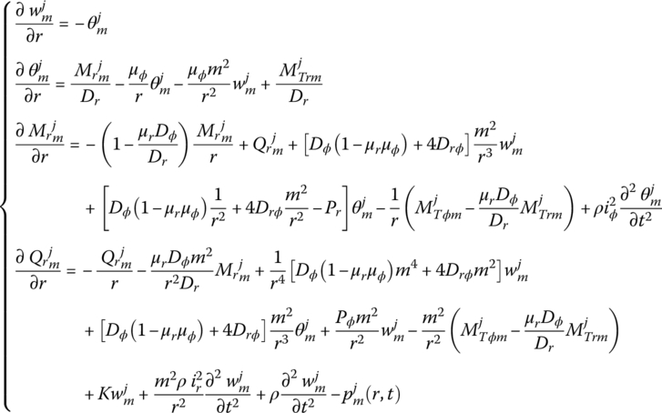
where ![]() or
or ![]() .
.
The state vector is defined as
The corresponding transfer matrix can be obtained as follows.
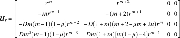
15.12.2 Massless Isotropic Disk
The transfer matrix is
-
 (15.66a)
-

- m ≥ 2

15.12.3 Massless Rigid Disk
The transfer matrix is
-
 (15.67a)
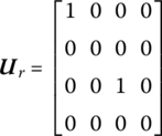
-
 (15.67b)
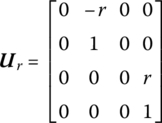
- m ≥ 2(15.67c)

15.12.4 Massless Disk with a Rigid Support at its Center
The transfer matrix is
-
 (15.68)
-

The transfer matrix can be obtained from Equation (15.66b) or Equation (15.66c).
15.12.5 Massless Disk with Planar Symmetrical Pressure Pr
The transfer matrix is

where J0(αr) and J1(αr) are the Bessel functions and ![]() .
.
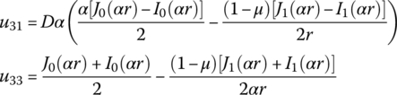
15.12.6 Symmetrical Disk
The transfer matrix is
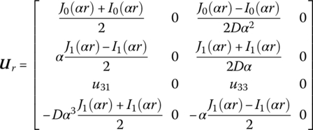
where
15.13 Strip Element of a Two‐dimensional Thin Plate
15.13.1 Massless Beam Strip
The beam strip i in a two‐dimensional plate, as shown in Figure 15.9, comprises m massless elastic beams. The state vectors of its input and output ends are defined as
where
Figure 15.9 The beam strips in a two‐dimensional plate.
The sequence number of the row of beam element (i, j) is denoted by index j, ![]() .
.
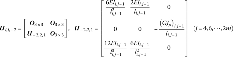
The transfer equation of the beam strip i is
The transfer matrix is
where
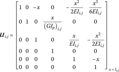
![]() is the transfer matrix of single beam element (i, j), and EIi,j, li,j and (GJp)i,j are the bending stiffness, length and torsional stiffness of the beam element (i, j), respectively.
is the transfer matrix of single beam element (i, j), and EIi,j, li,j and (GJp)i,j are the bending stiffness, length and torsional stiffness of the beam element (i, j), respectively.
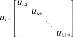
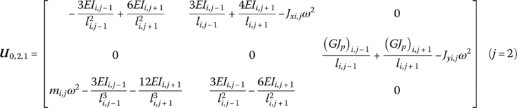
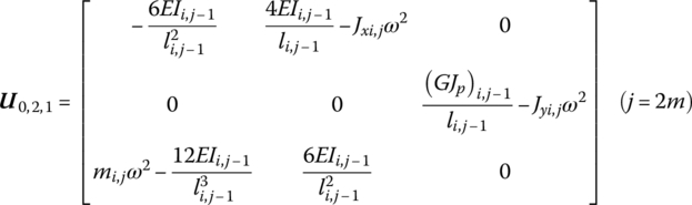
15.13.2 Lumped Mass Strip
The lumped mass strip i in a two‐dimensional plate, as shown in Figure 15.10, comprises m lumped masses and ![]() massless beams. The state vectors of its input and output ends are defined as
massless beams. The state vectors of its input and output ends are defined as
where

Figure 15.10 The lumped mass strips in a two‐dimensional plate.
The sequence number of the row of lumped mass element (i, j) is denoted by index j.
The transfer equation of the lumped mass strip i is
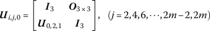
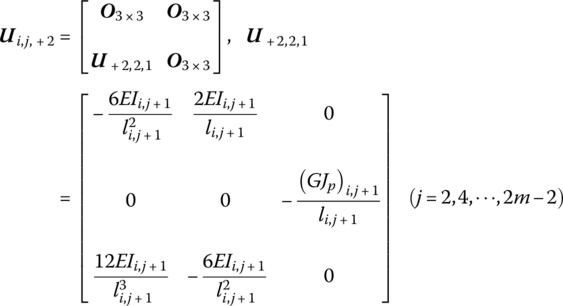
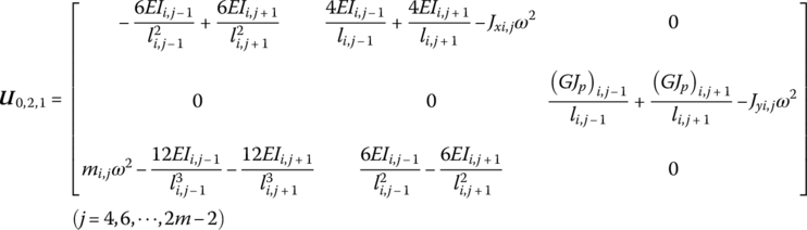
The transfer matrix is
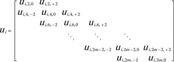
where
If the beam element (i, j) has a simply supported boundary, when ![]() and
and ![]() , we obtain
, we obtain

If the beam element (i, j) has a fixed boundary, when ![]() and
and ![]() ,
, ![]() in Equation (15.86) can be determined by Equation (15.87).
in Equation (15.86) can be determined by Equation (15.87).
If the beam element (i, j) has a free boundary, when ![]() and
and ![]() ,
,

15.14 Thick‐walled Cylinder
15.14.1 Dynamic Equations of a Thick‐walled Cylinder
As shown in Figure 15.11, the basic equations [38] for the radial motion of a thick‐walled cylinder are

where
r and ϕ are the radial coordinate and the circumferential coordinate. u is the radial displacement, σr is the radial stress, σϕ is the shear stress, pr is the distributed radial loading intensity, ρ is the mass density, α is the heat expansion coefficient, ΔT is the temperature variation, G is the material shear elastic modulus, λ is the Reynolds coefficient, E is the material elastic modulus and μ is the material Poisson’s ratio.
Figure 15.11 Positive radial displacement and stress.
The state vector is defined as
The corresponding transfer matrix can be obtained as follows.
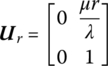
15.14.2 Massless Isotropic Cylinder
The transfer matrix is
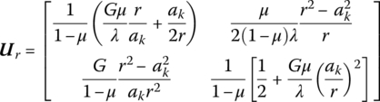
where ak is the radial coordinate of the inner surface of the cylinder.
15.14.3 Massless Isotropic Cylinder without a Center Hole
The transfer matrix is
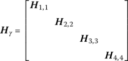
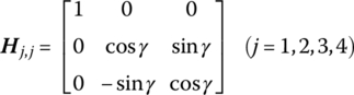
15.14.4 Isotropic Cylinder
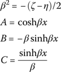
The transfer matrix is
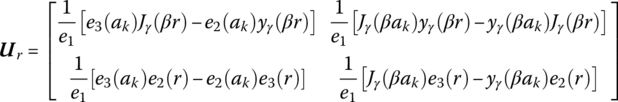
where
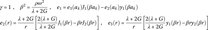
Jγ(βr) and yγ(βr) are the first type and second type of Bessel functions with λ, respectively.
15.14.5 Isotropic Cylinder without a Center Hole
The transfer matrix is
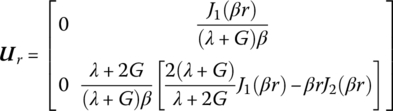
where ![]() and J1(βr), J2(βr) are the first kind Bessel functions.
and J1(βr), J2(βr) are the first kind Bessel functions.
15.15 Thin‐walled Cylinder
15.15.1 Dynamic Equations of a Thin‐walled Cylinder
As shown in Figure 15.12, the basic equations [38] for the radial motion and flexural displacement of a thin‐walled cylinder are
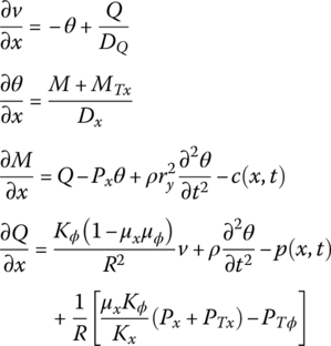
where x and ϕ are the axial coordinate and the circumferential coordinate, v is the radial displacement, θ is the rotational angle of the displacement course, R is the radius of the cylinder, M is the axial moment per unit circumferential length, Q is the shear force per unit circumferential length, DQ is the shear stiffness, Kx and Kϕ are the extention stiffnesses, Dx and Dϕ are the flexural stiffnesses, p and c are the distributed loading intensities, ρ is the mass density, μx and μϕ are the Poisson ratios of the material, ry is the gyration radius of the cross‐section around the y axis, Px is the axial pressure, and PTx and PTϕ are the temperature effect forces.
Figure 15.12 Positive deflection, internal moment and internal force.
For an isotropic homogeneous material
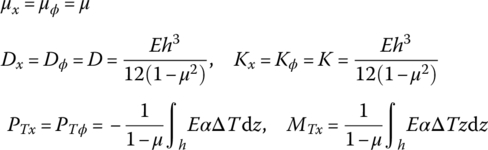
where α is the heat expansion coefficient, ΔT is the temperature variation and E is the material elastic modulus.
The state vector is defined as
The corresponding transfer matrix can be obtained as follows.
15.15.2 Massless Thin‐walled Cylinder with Shear Deformation
The transfer matrix is
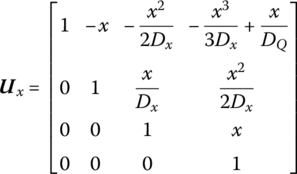
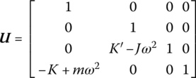
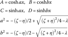
15.15.3 General Thin‐walled Cylinder
The transfer matrix is
where
e0, e1, e2, e3 and e4 are shown in Table 15.3.
Table 15.3 The expression of e0, e1, e2, e3 and e4
| e0 |
|
0 |
|
|
|
|
| e1 |
|
1 | A |
|
|
|
| e2 |
|
x | B |
|
|
|
| e3 |
|
|
|
|
|
|
| e4 |
 |
|
|
|
 |
 |
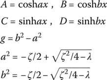
A, B, C, D, g, a and b in Table 15.3 are shown in Table 15.4.
Table 15.4 The expression of A, B, C, D, g, a and b
 |
 |
 |
 |
 |
 |
 |
 |
||
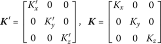
15.16 Coordinate Transformation Matrix
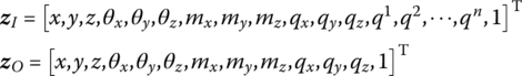
For convenient study, the inertial coordinate system describing the motion of each element may have different orientations. For instance, elements i and i + 1 are adjacent elements in a system. There is an angle between the coordinate system of element i and coordinate system i + 1, and the angle is denoted as ϕ. The state vector of the output end of element i described in the coordinates of element i is ![]() , and the state vector of the input end of element
, and the state vector of the input end of element ![]() described in the coordinates of element
described in the coordinates of element ![]() is
is ![]() . The state vector
. The state vector ![]() is often described in the coordinates of element
is often described in the coordinates of element ![]() , that is,
, that is, ![]() . However,
. However, ![]() and
and ![]() are also the same state vectors, but are described in different coordinate systems. The relation between them is
are also the same state vectors, but are described in different coordinate systems. The relation between them is
where ![]() is the coordinate transformation matrix corresponding to the angle ϕ between the two coordinates.
is the coordinate transformation matrix corresponding to the angle ϕ between the two coordinates.
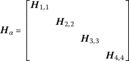
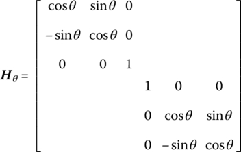
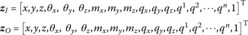
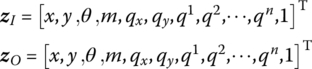
When spatial motion is studied, the state vector is defined as
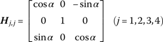
The three types of coordinate transform matrix that could be used are shown in Figure 15.13.
- Rotation about the x axis with angle γ(15.104)where
- Rotation about the y axis with angle α(15.105)where
- Rotation about the z axis with angle θ(15.106)where
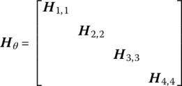
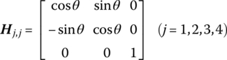
Figure 15.13 Coordinate transformation in space.
If planar motion is studied, as shown in Figure 15.14, the state vector can be defined as
Figure 15.14 Coordinate transformation in a plane.
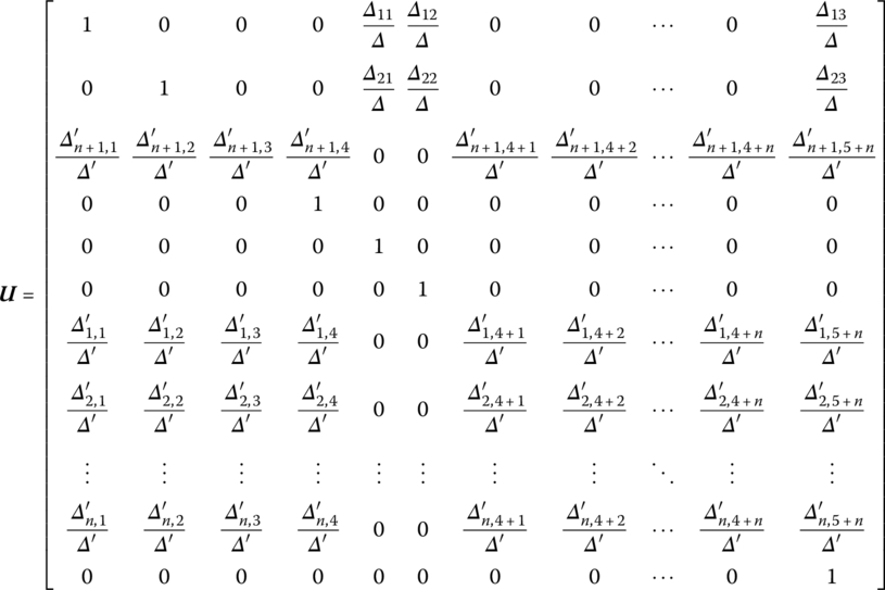
The coordinate transformation matrix is
If the form of the state vector is
the coordinate transformation matrix is

15.17 Linearization and State Vectors
15.17.1 Linearization
- Linearization of velocity (angular velocity) and acceleration (angular acceleration) leads to

According to the different numerical integration methods, the choices of
 ,
,  ,
,  and
and  are shown in Table 7.2.
 - Linearization of nonlinear functions
See Table 7.3.
- Linearization of the coordinate transformation matrix
The direction cosine matrix may be given as rotations about the spatially fixed three axes
 . Thus the angular velocity vector in the body‐fixed reference system is
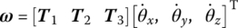
The linearization of the direction cosine matrix is
where
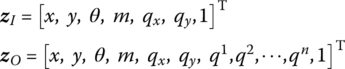
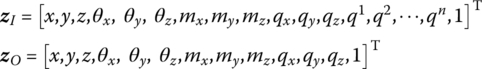
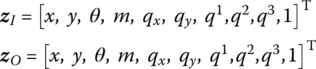
15.17.2 State Vectors
- Planar rigid body(15.111)
- Spatial rigid body(15.112)

- Planar beam(15.113)

- Spatial beam(15.114)

15.18 Spring and Damper Hinges Connected to Rigid Bodies
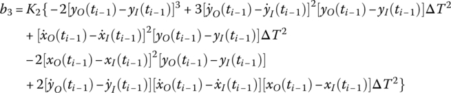
15.18.1 Spring Hinge whose Inboard and Outboard Bodies are Planar Rigid Bodies
Neglecting the mass and the initial length of the spring, the constitutive relationships of the nonlinear spring hinge are
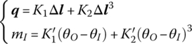
where ![]() is a variable quantity of the length of the spring and
is a variable quantity of the length of the spring and ![]() is the elastic force. K1 and K2 are the longitudinal stiffness coefficients of the nonlinear translational spring, and
is the elastic force. K1 and K2 are the longitudinal stiffness coefficients of the nonlinear translational spring, and ![]() and
and ![]() are the torsional stiffness coefficients of the nonlinear rotational spring.
are the torsional stiffness coefficients of the nonlinear rotational spring.
The transfer matrix is

where
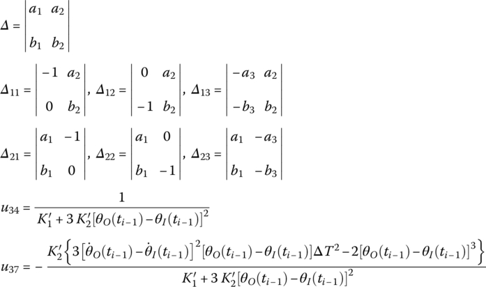
a1, a2, a3, b1, b2 and b3 are the linearization coefficients, as shown in Equation (8.199).
15.18.2 Damper Hinge whose Inboard and Outboard Bodies are Planar Rigid Bodies
For a viscous damper hinge whose inboard body and outboard body are planar rigid bodies, the damper force and damper torques are
where Cd and ![]() are the translational and rotary damper coefficients of dampers.
are the translational and rotary damper coefficients of dampers.
The transfer matrix is
where
C, ![]() ,
, ![]() ,
, ![]() ,
, ![]() ,
, ![]() and
and ![]() are the linearlization coefficients.
are the linearlization coefficients.
15.18.3 Spring and Damper Hinge whose Inboard and Outboard Bodies are Spatial Rigid Bodies
The transfer matrix is

where
15.19 Smooth Hinges Connected to Rigid Bodies
The transfer matrix of a smooth pin hinge whose outboard body also has a smooth pin hinge at its output is given as follows. The transfer matrix of a smooth pin hinge whose outboard hinge is neither a smooth ball‐and‐socket hinge nor a dummy hinge can be derived the method given in section 7.6.3.
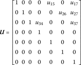
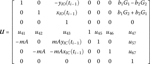
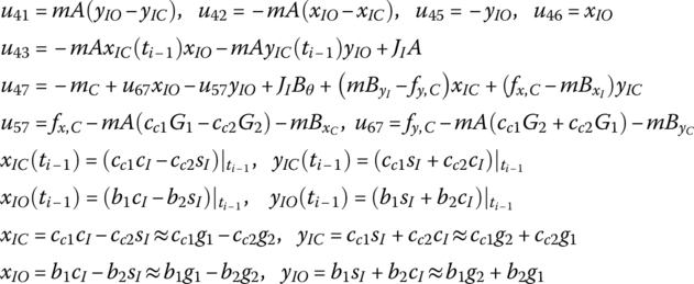
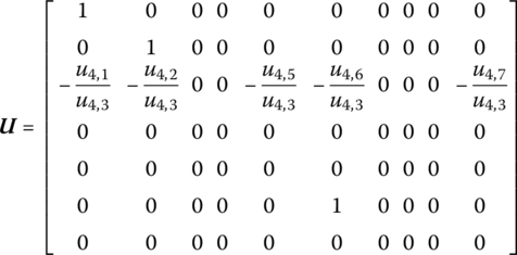
15.19.1 Smooth Pin Hinge whose Inboard and Outboard Bodies are Planar Rigid Bodies
The transfer matrix is
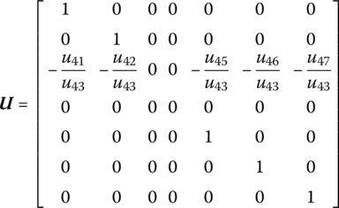
where u41, u42, u43, u45, u46 and u47 are elements of the transfer matrix of the outboard rigid body.
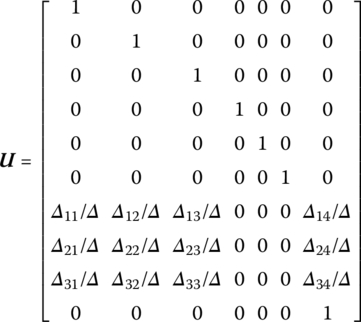
15.19.2 Smooth Ball‐and‐socket Hinge whose Inboard and Outboard Bodies are Spatial Rigid Bodies
The transfer matrix is
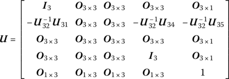
where ![]() are elements of the transfer matrix of the outboard rigid body.
are elements of the transfer matrix of the outboard rigid body.
15.20 Rigid Bodies Moving in a Plane
15.20.1 Rigid Body with One Input End and One Output End Moving in a Plane
The transfer matrix is
where
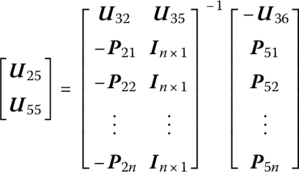
15.20.2 Planar Rigid Body with Multiple Input and Multiple Output Ends
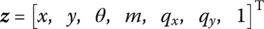
The state vector is
The transfer equation is
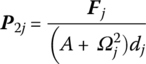
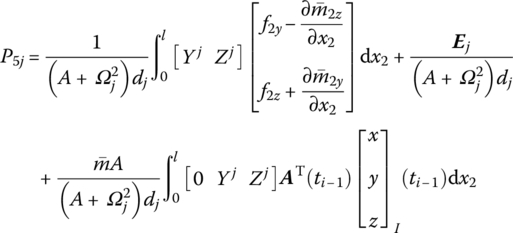
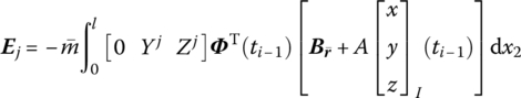
The transfer matrix is
Where

15.20.3 Planar Rigid Body with Multiple Input Ends and One Output End
The state vector is
The transfer equation is
The transfer matrix is
where the submatrices are the same as in Equation (15.102).
15.20.4 Planar Rigid Body with One Input End and Multiple Output Ends
The state vector is
The transfer equation is
The transfer matrix is
where the submatrices are the same as those in Equation (15.123).
15.21 Spatial Rigid Bodies with Large Motion and Various Connections
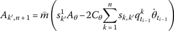
15.21.1 Spatial Rigid Body with One Input End and One Output End
The transfer equation is
The transfer matrix is
where
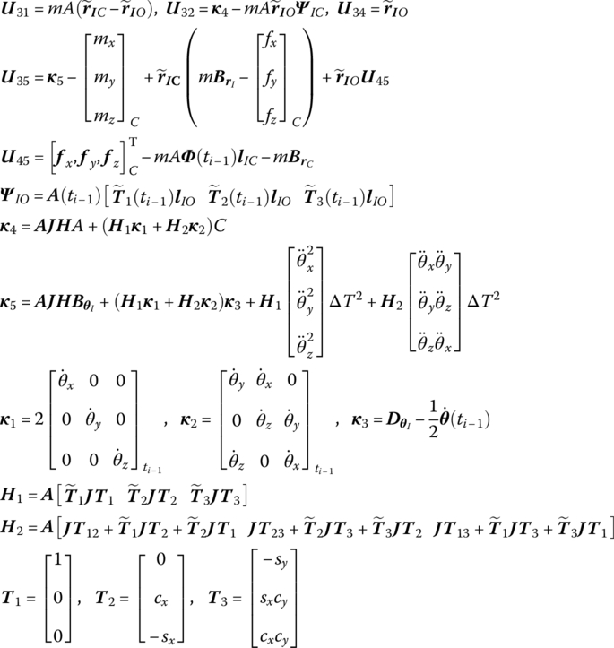
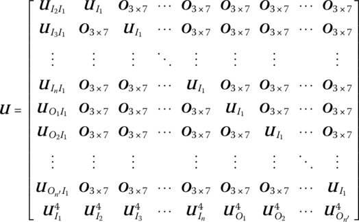
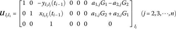
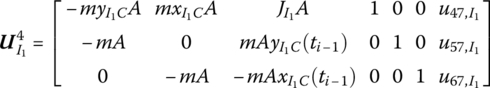
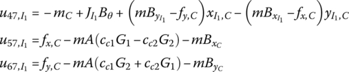
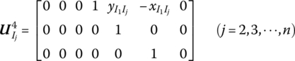
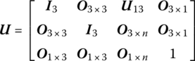
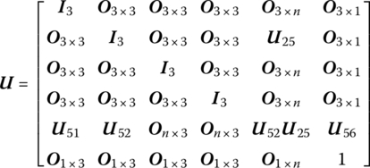
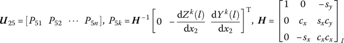
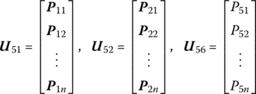
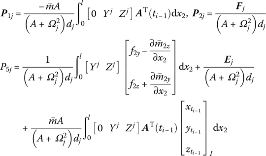
15.21.2 Spatial Rigid Body with Multiple Input and Multiple Output Ends
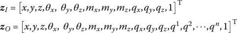
The state vector is
The transfer equation is
The transfer matrix is
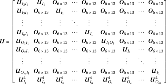
where
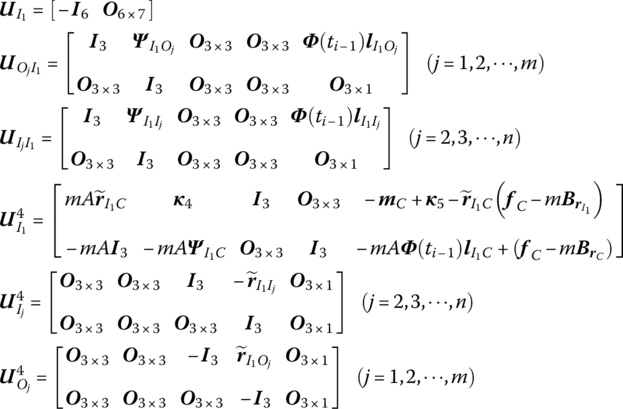
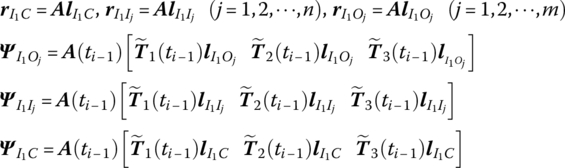
![]() is determined by Equation (7.84),
is determined by Equation (7.84), ![]() are determined by Equation (7.77), and m is the mass of the rigid body. fC is an external force acting on the mass center of the rigid body.
are determined by Equation (7.77), and m is the mass of the rigid body. fC is an external force acting on the mass center of the rigid body.
15.21.3 Spatial Rigid Body with Multiple Input Ends and One Output End
The state vector is
The transfer equation is
The transfer matrix is
where the submatrices are the same as in Equation (15.134).
15.21.4 Spatial Rigid Body with One Input End and Multiple Output Ends
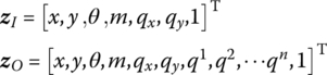
The state vector is
The transfer equation is
The transfer matrix is
where the submatrices are the same as in Equation (15.134).
15.22 Planar Beam with Large Motion
The state vector is
The transfer equation is
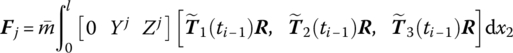
The transfer matrix is
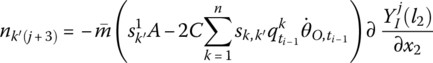
where
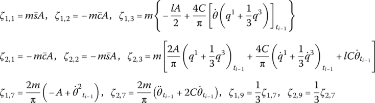
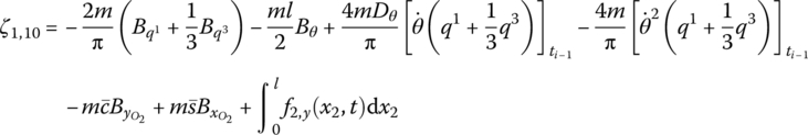

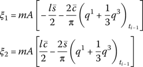


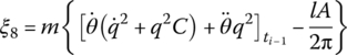
f2,x and f2,y are distributing external forces with respect to the body‐fixed coordinate system, and m′ is the distributed external torque acting on the beam. ![]() and
and ![]() are determined by Equation (7.62).
are determined by Equation (7.62).
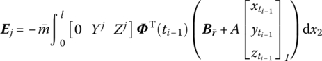
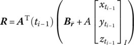
15.23 Spatial Beam with Large Motion
The state vector is
The transfer equation is
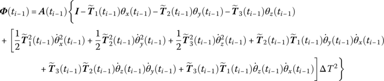
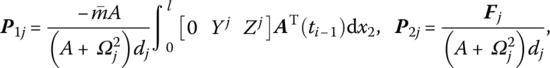
The transfer matrix is
where


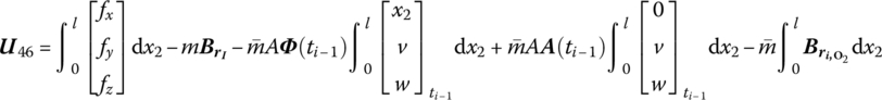
![]() is determined by Equation (7.84),
is determined by Equation (7.84), ![]() are determined by Equation (7.77),
are determined by Equation (7.77), ![]() is the coordinate transform matrix, EI, l and
is the coordinate transform matrix, EI, l and ![]() are the bending stiffness, length and line density of the beam, respectively, Yk(x2) and Zk(x2) are the eigenvectors of outboard beam, and
are the bending stiffness, length and line density of the beam, respectively, Yk(x2) and Zk(x2) are the eigenvectors of outboard beam, and ![]() and
and ![]() are determined by Equation (7.62).
are determined by Equation (7.62).
15.24 Fixed Hinges Connected to a Planar Beam with Large Motion
15.24.1 Fixed Hinge whose Inboard Body is a Rigid Body and whose Outboard Body is a Euler–Bernoulli Beam Moving in a Plane
The state vectors are
The transfer equation is
The transfer matrix is
where all elements are the same as in Equation (8.135).
15.24.2 Fixed Hinge whose Inboard and Outboard Bodies are Euler–Bernoulli Beams Moving in a Plane
The state vectors are
The transfer equation is
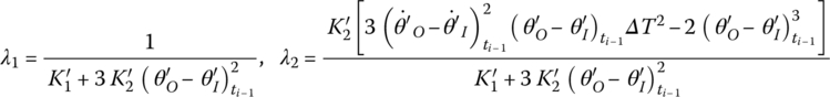
The transfer matrix is

where
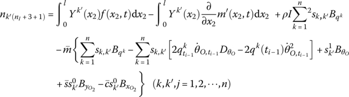
θO is the orientation angle of the output end of the fixed hinge, that is, the orientation angle of the body‐fixed coordinate system of its outboard beam. ![]() is the eigenvector of the inboard beam. The n is the highest order of the modes of the beam connected with the fixed hinge. The other elements are the parameters of the outboard beam, and their meanings are the same as in Equation (8.116).
is the eigenvector of the inboard beam. The n is the highest order of the modes of the beam connected with the fixed hinge. The other elements are the parameters of the outboard beam, and their meanings are the same as in Equation (8.116).
15.24.3 Fixed Hinge whose Inboard Body is a Euler–Bernoulli Beam and whose Outboard Body is a Rigid Body Moving in a Plane
The state vectors are
The transfer equation is
The transfer matrix is
where the meanings of all the elements are the same as in Equation (8.135).
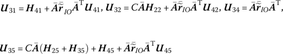
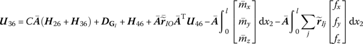
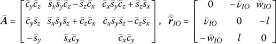
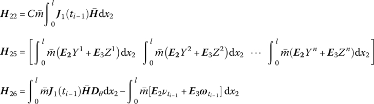
15.25 Fixed Hinges Connected to a Spatial Beam with Large Motion
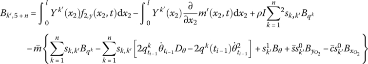
15.25.1 Fixed Hinge whose Inboard Body is a Rigid Body and whose Outboard Body is a Beam Moving in Space
The state vectors are
The transfer equation is
The transfer matrix is

where

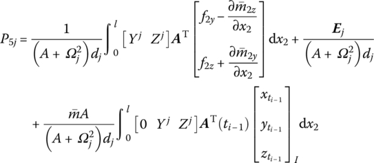


![]() is the kth natural frequency,
is the kth natural frequency, ![]() is determined by Equation (7.84),
is determined by Equation (7.84), ![]() are determined by Equation (7.77), and
are determined by Equation (7.77), and ![]() is the coordinate transform matrix. EI, l and
is the coordinate transform matrix. EI, l and ![]() are the bending stiffness, length and mass per unit length of the beam, respectively.
are the bending stiffness, length and mass per unit length of the beam, respectively. ![]() and
and ![]() (f2z and f2y) are distributing external torques (forces) with respect to the body‐fixed coordinate system. Yj(x2) and Zj(x2) are the eigenvectors of the outboard beam.
(f2z and f2y) are distributing external torques (forces) with respect to the body‐fixed coordinate system. Yj(x2) and Zj(x2) are the eigenvectors of the outboard beam.
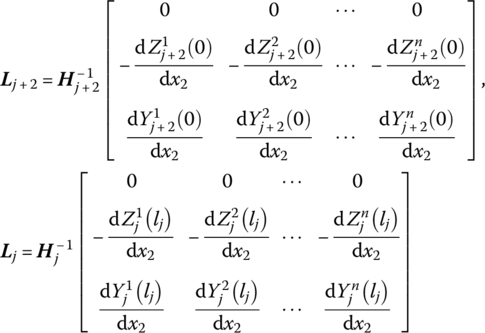
15.25.2 Fixed Hinge whose Inboard and Outboard Bodies are Euler–Bernoulli Beams Moving in Space
The state vectors are

The transfer equation is
The transfer matrix is
where


Ωk is the kth natural frequency, ![]() is determined by Equation (7.84),
is determined by Equation (7.84), ![]() are determined by Equation (7.77), and
are determined by Equation (7.77), and ![]() is the coordinate transform matrix. EI, l and
is the coordinate transform matrix. EI, l and ![]() are the bending stiffness, length and mass per unit length of the beam, respectively. Yj(x2) and Zj(x2) are the eigenvectors of the outboard beam. f2z and f2y (
are the bending stiffness, length and mass per unit length of the beam, respectively. Yj(x2) and Zj(x2) are the eigenvectors of the outboard beam. f2z and f2y (![]() and
and ![]() ) are distributing external forces (torques) with respect to the body‐fixed coordinate system.
) are distributing external forces (torques) with respect to the body‐fixed coordinate system.
15.25.3 Fixed Hinge whose Inboard Body is a Euler–Bernoulli Beam and whose Outboard Body is a Rigid Body Moving in Space
Deleting the row elements corresponding to generalized coordinates in Equation (15.161), the transfer equation and transfer matrix of a fixed hinge whose inboard body is a beam and whose outboard body is a rigid body moving in space can be obtained.
The state vectors are
The transfer equation is
The transfer matrix is

where the meanings of all the elements are the same as in Equation (15.161).
15.26 Smooth Hinges Connected to a Beam with Large Planar Motion
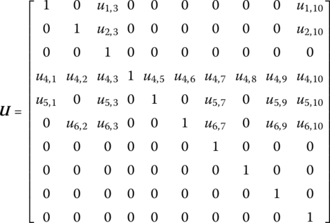
15.26.1 Smooth Hinge whose Inboard and Outboard Bodies are Euler–Bernoulli Beams Moving in a Plane
The state vectors are
The transfer equation is
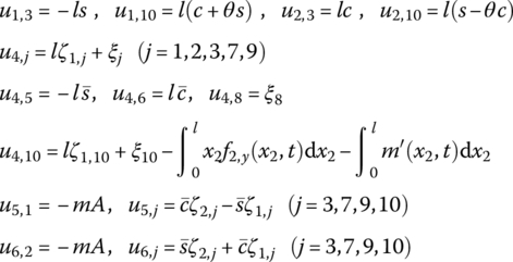
The transfer matrix is
where
u4,1, u4,2, ![]() , u4,10 are the elements of the transfer matrix of the outboard beam. EI is the bending stiffness of the beam,
, u4,10 are the elements of the transfer matrix of the outboard beam. EI is the bending stiffness of the beam, ![]() is the mass per unit length of the beam and l is the length of the beam. f2,y(x2, t) are the distributed external forces acted on the beam in the y2 direction and m′ is the distributed external torque acted on the beam.
is the mass per unit length of the beam and l is the length of the beam. f2,y(x2, t) are the distributed external forces acted on the beam in the y2 direction and m′ is the distributed external torque acted on the beam. ![]() and
and ![]() are determined by Equation (7.62).
are determined by Equation (7.62).
15.26.2 Smooth Hinge whose Inboard Body is a Rigid Body and whose Outboard Body is a Euler–Bernoulli Beam Moving in a Plane
The state vectors are
The transfer equation is
The transfer matrix is
where the meanings of all the elements are the same as in Equation (15.167).
15.26.3 Smooth Pin Hinge whose Inboard Body is a Euler–Bernoulli Beam and whose Outboard Body is a Rigid Body Moving in a Plane
The state vectors are
The transfer equation is
The transfer matrix is
where the meanings of all the elements are the same as in Equation (7.219).
15.27 Smooth Hinges Connected to a Beam with Large Spatial Motion
15.27.1 Smooth Ball‐and‐socket Hinge whose Inboard Body is a Rigid Body and whose Outboard Body is a Euler–Bernoulli Beam Moving in Space
The state vectors are
The transfer equation is
The transfer matrix is
where

Ωk is the kth natural frequency, ![]() is determined by Equation (7.84),
is determined by Equation (7.84), ![]() are determined by Equation (7.77) and
are determined by Equation (7.77) and ![]() is the coordinate transform matrix. l and
is the coordinate transform matrix. l and ![]() are the length and mass per unit length of the beam, respectively. Yj(x2) and Zj(x2) are the eigenvectors of the outboard beam. f2z and f2y (
are the length and mass per unit length of the beam, respectively. Yj(x2) and Zj(x2) are the eigenvectors of the outboard beam. f2z and f2y (![]() and
and ![]() ) are distributing external forces (torques) with respect to the body‐fixed coordinate system.
) are distributing external forces (torques) with respect to the body‐fixed coordinate system.
15.27.2 Smooth Ball‐and‐socket Hinge whose Inboard and Outboard Bodies are Euler–Bernoulli Beams Moving in Space
The state vectors are
The transfer equation is
The transfer matrix is
where the meanings of all the elements are the same as in Equation (15.176).
15.27.3 Smooth Ball‐and‐socket Hinge whose Inboard Body is a Euler–Bernoulli Beam and whose Outboard Body is a Rigid Body Moving in Space
The state vectors are
The transfer equation is
The transfer matrix is
where the meanings of all the elements are the same as in Equation (15.176).
15.28 Elastic Hinges Connected to a Beam with Large Planar Motion
15.28.1 Elastic Hinge whose Inboard and Outboard Bodies are Beams Moving in a Plane
The state vectors are
The transfer equation is
The transfer matrix is
where

For example


K1 and K2 are the stiffness coefficients of the nonlinear spring, ![]() and
and ![]() are the torsional stiffness coefficients of the nonlinear rotary spring. l is the length of the beam.
are the torsional stiffness coefficients of the nonlinear rotary spring. l is the length of the beam. ![]() is the mass per unit length of the beam, f2,y is the distributed external force acted on the beam in the y2 direction and m′ is the distributed external torque acted on the beam. Yk(x2) is the eigenvector of the outboard beam,
is the mass per unit length of the beam, f2,y is the distributed external force acted on the beam in the y2 direction and m′ is the distributed external torque acted on the beam. Yk(x2) is the eigenvector of the outboard beam, ![]() is the eigenvector of the inboard beam,
is the eigenvector of the inboard beam, ![]() and
and ![]() are determined by Equation (8.109), and
are determined by Equation (8.109), and ![]() and
and ![]() are determined by Equation (7.62).
are determined by Equation (7.62).
15.28.2 Elastic Hinge whose Inboard Body is a Rigid Body and whose Outboard Body is a Euler–Bernoulli Beam Moving in a Plane
The state vectors are
The transfer equation is
The transfer matrix is
where the meanings of all the elements are the same as in Equation (15.185). In the computation ![]() should be used.
should be used.
15.28.3 Elastic Hinge whose Inboard Body is a Euler–Bernoulli Beam and whose Outboard Body is a Rigid Body Moving in a Plane
The state vectors are
The transfer equation is
The transfer matrix is
where 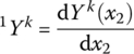 and the meanings of all the other elements are the same as in Equation (15.185).
15.29 Elastic Hinges Connected to a Beam Moving in Space
15.29.1 Elastic Hinge whose Inboard and Outboard Bodies are Euler–Bernoulli Beams Moving in Space
The state vectors are
The transfer equation is
The transfer matrix is
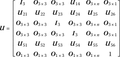
where ![]() is a
is a ![]() matrix and
matrix and ![]() is a
is a ![]() matrix.
matrix.
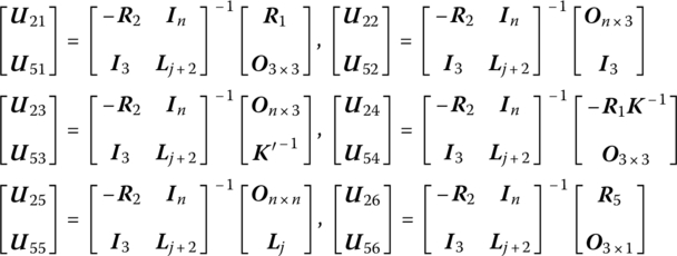
![]() have the same meaning as in Equation (8.191).
have the same meaning as in Equation (8.191). ![]() is the torsional stiffness of the rotary springs,
is the torsional stiffness of the rotary springs, ![]() is the stiffness of the springs, and Kx, Ky and Kz and
is the stiffness of the springs, and Kx, Ky and Kz and ![]() are the stiffness coefficients of the linear springs and the torsional stiffness coefficients of the rotary springs, respectively.
are the stiffness coefficients of the linear springs and the torsional stiffness coefficients of the rotary springs, respectively.
15.29.2 Elastic Hinge whose Inboard Body is a Rigid Body and whose Outboard Body is a Euler–Bernoulli Beam Moving in Space
The state vectors are
The transfer equation is
The transfer matrix is

where the meanings of all the elements are the same as in Equation (15.194).
15.29.3 Elastic Hinge whose Inboard Body is a Euler–Bernoulli Beam and whose Outboard Body is a Rigid Body Moving in Space
The state vectors are

The transfer equation is
The transfer matrix is
where the meaning of ![]() is the same as in Equation (9.227) and the meanings of
is the same as in Equation (9.227) and the meanings of ![]() and
and ![]() are the same as in Equation (9.223).
are the same as in Equation (9.223).
15.30 Controlled Elements of a Linear System
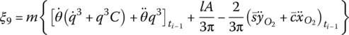
15.30.1 Vibration System under Real‐time Control
The controlled vibration system is shown in Figure 15.15. The system is mounted on the lumped mass k, where the controlled force acting on the displacement, velocity and acceleration of lumped mass k is

Figure 15.15 Vibration system under real‐time control.
The transfer equation of the lumped mass k under real‐time control can be obtained as
where
mp is the mass of the lumped mass p. Fp is a simple harmonic external force acting on the lumped mass p with frequency Ω.
15.30.2 Controlled Branched System
A controlled branched system is shown in Figure 9.32. The state vectors of each connection point are
![]() ,
, ![]() ,
, ![]() ,
, ![]() ,
, ![]() ,
, ![]() and
and ![]() have the same form as
have the same form as ![]() ,
, ![]() and
and ![]() have the same form as
have the same form as ![]() , and
, and ![]() ,
, ![]() ,
, ![]() ,
, ![]() and
and ![]() have the same form as
have the same form as ![]() .
.
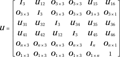
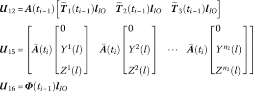
The overall transfer equation is
The state vector is
The transfer matrix is
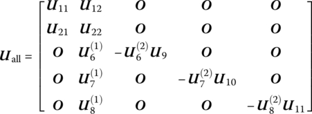
where
15.31 Controlled Elements of a General Time‐variable System
15.31.1 Vibration System under Real‐time Control
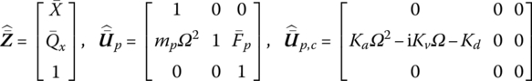
For the controlled vibration system shown in Figure 15.15, linearizing Equation (15.201) yields
The transfer equation of the controlled lumped mass p is
where
mp is the mass of the lumped mass p. Fp is the external force acting on the lumped mass p.
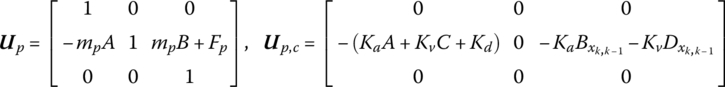
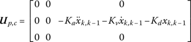
For the delay controlled system, the control force can be seen as an external force related to the previous time motion state. By adding the control force into the external force submatrix of the corresponding transfer matrix, the controlled system can be considered as a system without control. The control force Fp,c in Equation (15.201) is a function of the motion quantities ![]() ,
, ![]() and
and ![]() :
:
where τ is the delay time. Adding the control force Fp,c into the element u23 of the transfer matrix of the element p, we obtain
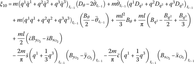
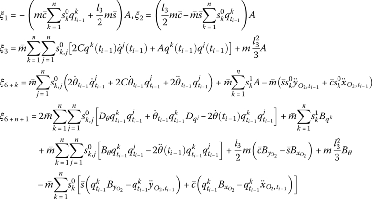
15.31.2 Controlled Flexible Manipulator System
The controlled planar flexible manipulator system assembled by hub 1 and flexible arm 3, featuring surface‐bonded piezoceramics and piezofilms, is shown in Figure 9.42a. m1, r1, ![]() ,
, ![]() and
and ![]() are the mass, gyration radius, moment of inertia, desired orientation angle and desired orientation angular velocity of the hub 1, respectively. θ1 and
are the mass, gyration radius, moment of inertia, desired orientation angle and desired orientation angular velocity of the hub 1, respectively. θ1 and ![]() are the actual orientation angle and actual angular velocity, respectively. EI3, A3, l3, b and tb are the bending stiffness, cross‐section area, length, width and thickness of flexible arm 3, respectively. Ea, la, ta and d31 are the piezoelectric elastic modulus, length, thickness and strain constant of the segmented piezoelectric ceramic (PZT) actuator. Kp and Kv are the proportional gain coefficient and velocity gain coefficient of the servomotors, respectively. τ0(t) is the control torque of the motor, Kai is the gain coefficient of the segmented PZT actuator, Vi is the driven voltage applied to segmented PZT actuator i and u is the deformation of the flexible arm. Yk(x2) is the kth generalized eigenvector describing the deformation of the flexible arm.
are the actual orientation angle and actual angular velocity, respectively. EI3, A3, l3, b and tb are the bending stiffness, cross‐section area, length, width and thickness of flexible arm 3, respectively. Ea, la, ta and d31 are the piezoelectric elastic modulus, length, thickness and strain constant of the segmented piezoelectric ceramic (PZT) actuator. Kp and Kv are the proportional gain coefficient and velocity gain coefficient of the servomotors, respectively. τ0(t) is the control torque of the motor, Kai is the gain coefficient of the segmented PZT actuator, Vi is the driven voltage applied to segmented PZT actuator i and u is the deformation of the flexible arm. Yk(x2) is the kth generalized eigenvector describing the deformation of the flexible arm. ![]() ,
, ![]() is the position of each piezofilm sensor/PZT on the corresponding flexible arm in the body‐fixed reference frames. Adopting the proportional‐differential (PD) controller and modal velocity feedback control on the PZT actuators, the transfer matrices of the rigid body and beam under control are derived as follows.
is the position of each piezofilm sensor/PZT on the corresponding flexible arm in the body‐fixed reference frames. Adopting the proportional‐differential (PD) controller and modal velocity feedback control on the PZT actuators, the transfer matrices of the rigid body and beam under control are derived as follows.
Considering only the control moment related to its feedback state, the transfer matrix of the rigid body under control can be obtained as

where
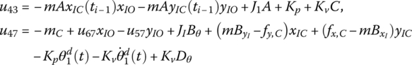
The meanings of u41, u42, u45, u46, u57 and u67 are the same as in Equation (7.101).
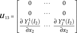
Considering the control moment of the PZT actuators, the transfer matrix of the beam under control is
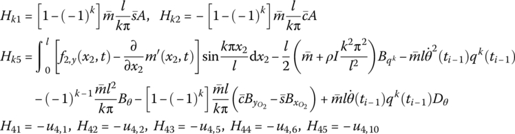
Where
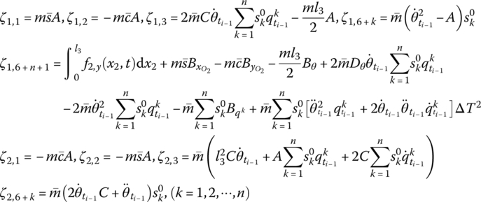
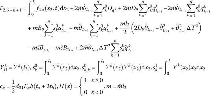
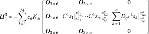
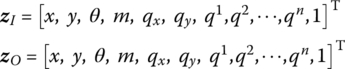
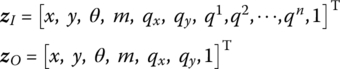
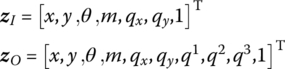
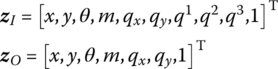
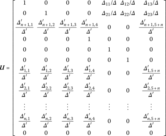
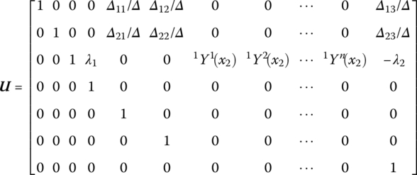
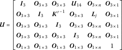
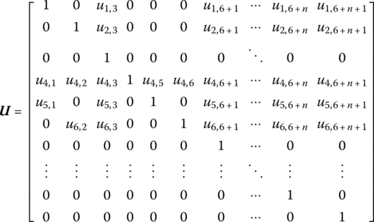
Considering the distributed moment of the PZT actuators, combining the control equation of PZT actuators and the numerical integration procedure, if the highest order of the modes considered is ![]() , then the state vectors of the fixed hinge connected to the beam under control can be defined as
, then the state vectors of the fixed hinge connected to the beam under control can be defined as
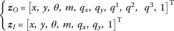
The transfer equation is
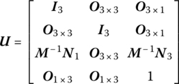
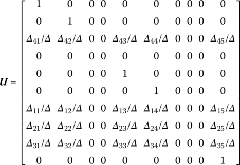
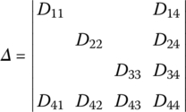
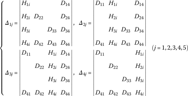
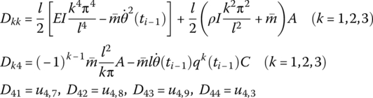
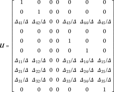
The transfer matrix is
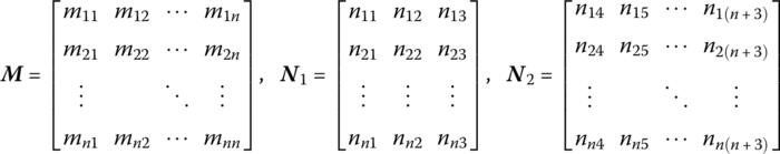
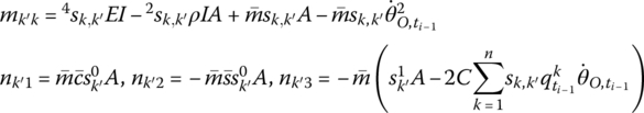
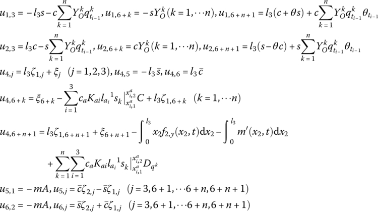
where

Adopting the PD controller and modal velocity feedback control on the PZT actuators, the transfer matrix ![]() of the equivalent control element is
of the equivalent control element is
where ![]() is the feedback parameter matrix related to the feedback from beam 3 to hub 1. For the modal velocity feedback control, that is
is the feedback parameter matrix related to the feedback from beam 3 to hub 1. For the modal velocity feedback control, that is