
CHAPTER 0
Overview
0.1 GLOBAL FIXED INCOME MARKETS
Fixed income markets are large and global. Figure 0.1 shows the outstanding amounts of debt securities, by residence of issuer. Debt securities are instruments designed to be traded, like bonds issued by corporations or by governments. Grouping by residence of issuer means, for example, that US Treasury bonds held by China's central bank are included in the total for the United States. As of March 2021, the global total of outstanding debt securities was about $123 trillion. For reference, the total capitalization of global equity markets at the time was $110 trillion, although stock market values are significantly more volatile.
Figure 0.1 shows that the five largest issuers, in terms of amounts outstanding, are in the United States, the Eurozone, China, Japan, and the United Kingdom, which together comprise nearly 90% of the total. The Eurozone includes countries that both belong to the European Union (EU) and use the euro as a national currency. Some individual members of the Eurozone, indicated with asterisks in the figure, are significant issuers of debt securities on their own. Note that the figure displays their amounts outstanding with gray bars, but their contributions to the cumulative total are included once, with the Eurozone total.
Figure 0.2 decomposes debt outstanding in the five largest regions by sector. The large fraction of government debt in Japan reflects decades of government borrowing and spending intended to stimulate the economy. The fraction of government debt in the United States, the Eurozone, and the United Kingdom is lower, at about 50%, but has increased significantly since the financial crisis of 2007–2009. Corporations in the United States are relatively more likely to issue bonds directly to the public, while corporations in the Eurozone, Japan, and the United Kingdom are relatively more likely to borrow funds from intermediaries, like banks, which, in turn, raise money from the public. While Figure 0.2 includes the breakdown for debt in China, the relatively large role of the government in financial and nonfinancial enterprises makes comparisons across sectors and regions less meaningful.
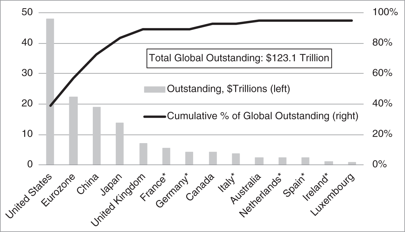
FIGURE 0.1 Global Debt Securities Outstanding, by Residence of Issuer, as of March 2021. Countries with an Asterisk Are in the Eurozone.
Sources: BIS; and Author Calculations.
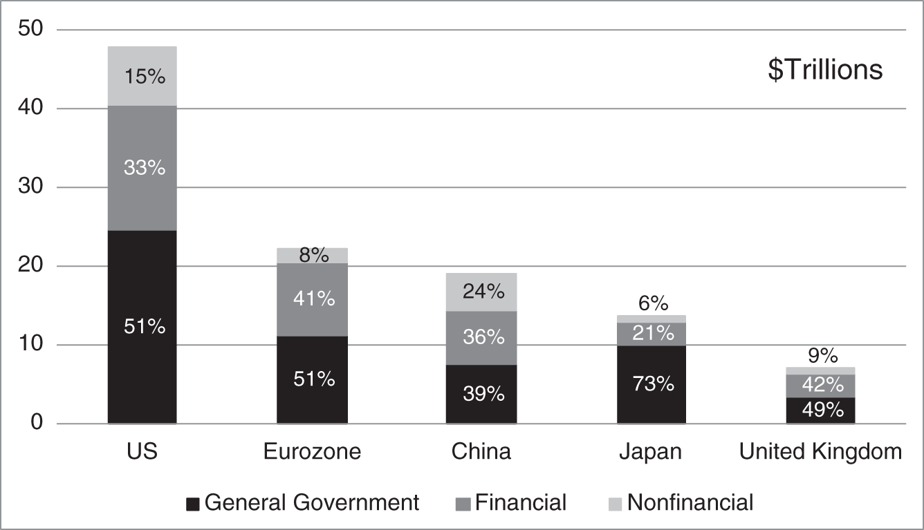
FIGURE 0.2 Global Debt Securities Outstanding, by Sector, as of March 2021.
Sources: BIS; and Author Calculations.
Table 0.1 and Figure 0.3 show the notional amounts of outstanding interest rate derivatives across the globe. These derivatives are described in later chapters, but derivatives essentially allow market participants to take positions on interest rates, whether for hedging, investment, or speculative purposes. The notional amount of a derivative is used to calculate the cash flows that one of the derivative's counterparties pays the other. Adding together all notional amounts, however, can significantly overstate market size. First, the largest market participants, namely dealers, tend to be simultaneously long and short nearly identical derivatives. Second, options are actually equivalent to only fractions of the notional amounts of their underlying securities. Later chapters elaborate on these points, but, for the purposes of this overview, this table and figure are reported in notional amounts.
While derivatives may trade in a particular locality, there is no sense in which derivatives are issued in one place or another: local regulations aside, any entity, residing anywhere, can enter into these derivatives contracts. A typical classification, therefore, is the currency in which the cash flows of the derivative are denominated. The first two columns of Table 0.1 show notional amounts for swaps, options, and forward rate agreements. Most of the outstanding amounts are denominated in US Dollars (USD) and Euro (EUR). The quantities in the table hint at the overstatement of market size by notional amount: if the sizes of the markets for these USD derivatives were really $150 trillion, they would be larger than the combined size of all global debt securities markets. The second two columns of the table show the notional amounts of standardized, exchange‐traded interest rate futures and options. Amounts outstanding of USD‐denominated contracts are by far the greatest, with those denominated in British Pounds (GBP) and EUR making up most of the rest of the overall market.
TABLE 0.1 Notional Amounts of Interest Rate Derivatives. Swaps, Options, and FRAs, as of June 2020; Futures and Futures Options, as of December 2020. Entries in $Trillions.
| Swaps, Options, FRAs | Futures and Futures Options | ||
|---|---|---|---|
| Currency | Amount | Currency | Amount |
| USD | 152.1 | USD | 41.5 |
| EUR | 132.6 | GBP | 10.4 |
| Other | 67.1 | EUR | 9.5 |
| GBP | 54.3 | BRL | 1.6 |
| JPY | 37.1 | CAD | 1.0 |
| CAD | 14.3 | AUD | 0.9 |
| SEK | 5.3 | Other | 0.6 |
| CHF | 3.6 | ||
USD: United States Dollar; EUR: Euro; GBP: British Pound; JPY: Japanese Yen; CAD: Canadian Dollar; SEK: Swedish Krona; CHF: Swiss Franc; BRL: Brazilian Real; AUD: Australian Dollar.
Source: BIS.
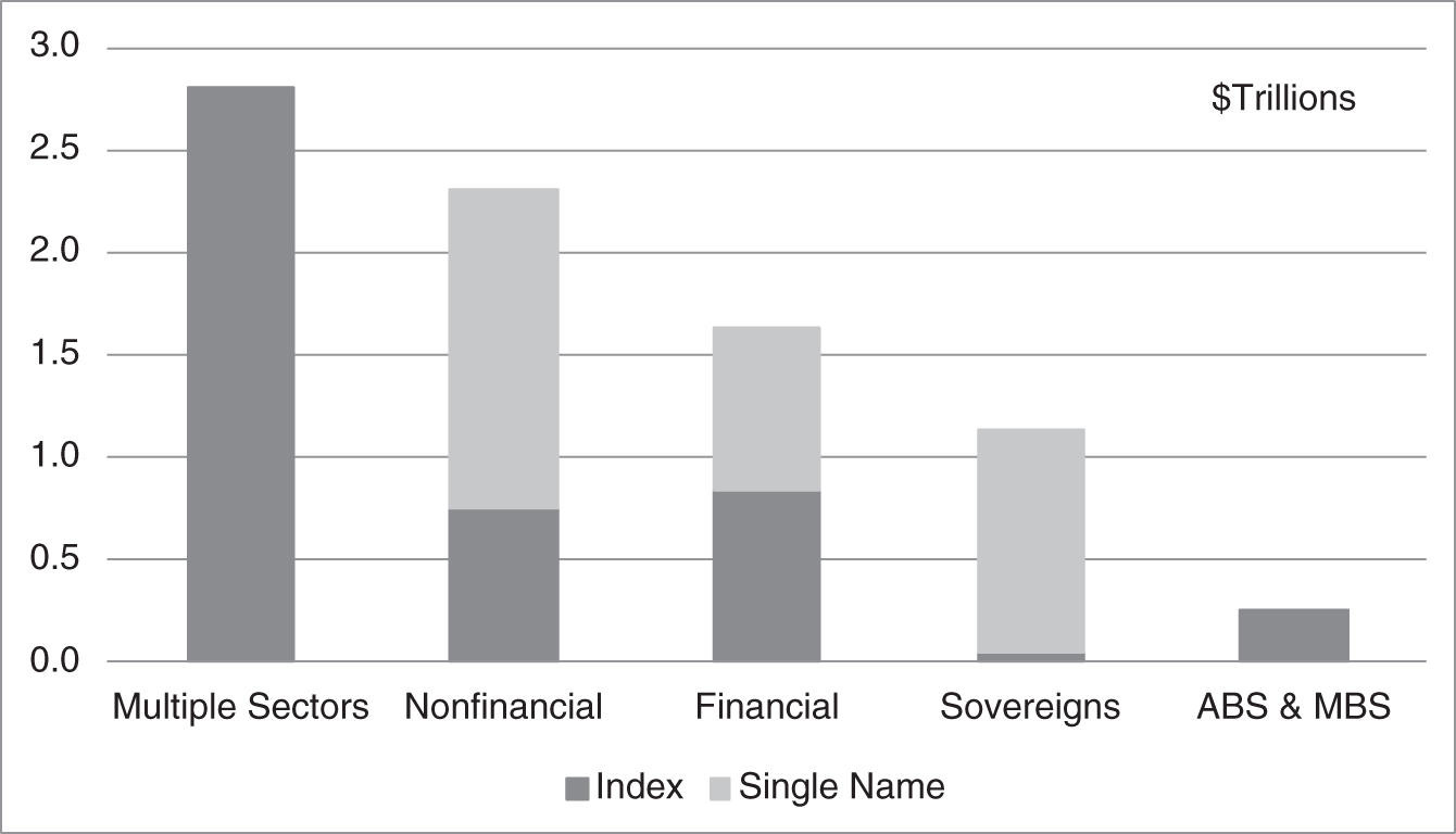
FIGURE 0.3 Credit Default Swaps, Notional Amounts Outstanding, by Sector and Type, as of June 2020.
Source: BIS.
Finally, Figure 0.3 gives the notional amount of credit default swaps (CDS) outstanding. These are discussed in detail in Chapter 14, but, roughly speaking, CDS allow investors to take positions that are equivalent to leveraged long or short positions in bonds with credit risk. The figure divides the market into credit sectors: CDS can be written on nonfinancial companies, financial companies, sovereigns, asset‐backed securities (ABS), and mortgage‐backed securities (MBS). Within each sector, a single‐name CDS references a single credit (e.g., the government of Spain), while an index CDS references a portfolio of credits (e.g., 25 European financial companies). Note that the CDS market is much smaller in notional amount than the derivatives markets depicted in Table 0.1.
0.2 US MARKETS
This section describes debt and loan instruments in the United States, categorized as in Figure 0.4. The total amount outstanding across all instruments, as of June 2021, was $76.4 trillion.1 By way of comparison, the market capitalization of US equities at the same time was about $45 trillion. Treasury securities and municipal securities are discussed in this section in some detail, while sectors discussed in later chapters of the book are treated very briefly here.
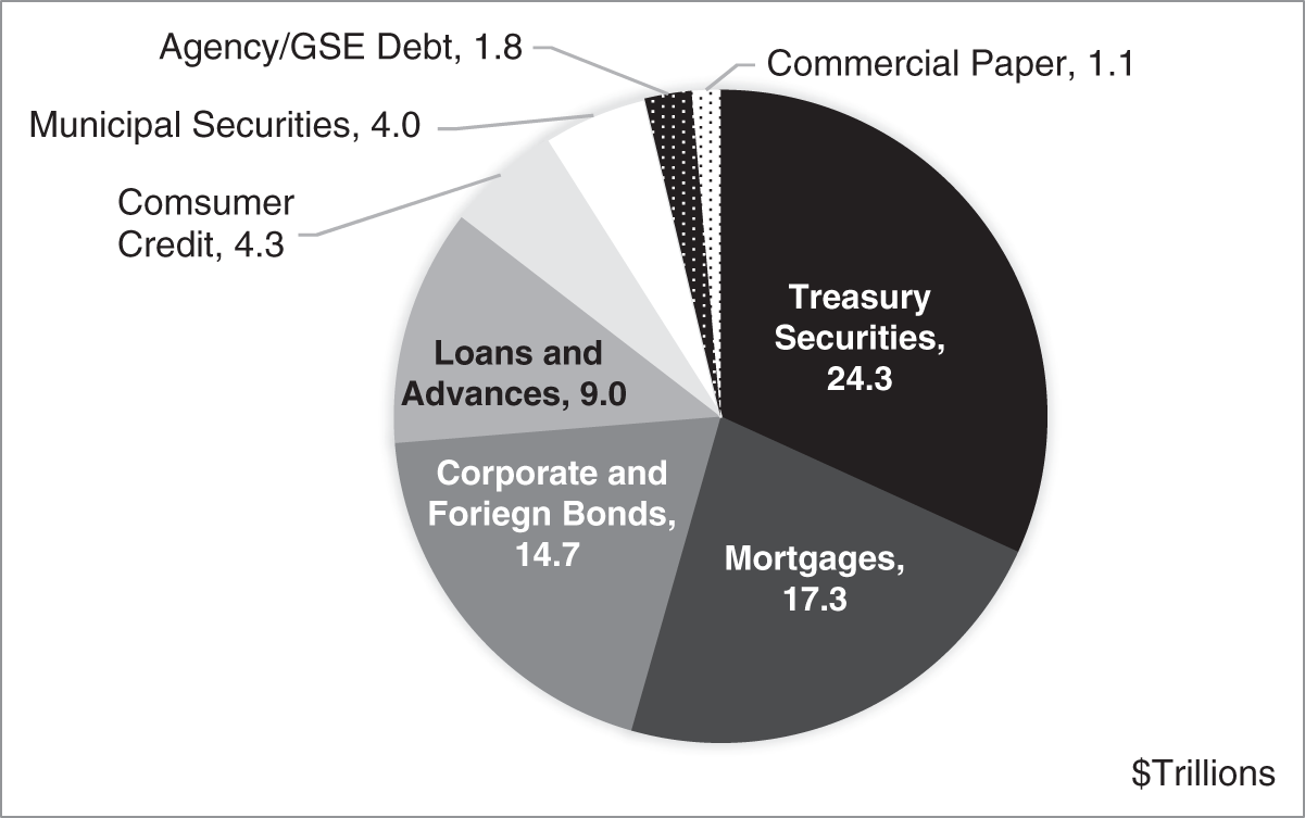
FIGURE 0.4 Debt Securities and Loans in the United States, Amounts Outstanding, as of June 2021. GSE: Government‐Sponsored Enterprise.
Sources: Financial Accounts of the United States, Board of Governors of the Federal Reserve System; and Author Calculations.
Treasury Securities
In less than a decade, Treasury securities have grown from the third largest category, behind mortgages and corporate and foreign bonds, to the largest category, at $24.3 trillion. When the US government spends more than it collects in taxes and fees, which has been the case for most of the last 50 years, it needs to borrow money to fund its deficit spending. It does so through the array of instruments shown in Figure 0.5. Treasury bills or T‐bills mature in one year or less and are discount securities, which means that they sell for less than, or at a discount from, their promised payment at maturity. Treasury notes and bonds are coupon‐bearing securities; that is, they earn a fixed coupon or interest rate on their principal, face, or par amounts through maturity, and then repay that principal amount at maturity. Strictly speaking, and in the accounts of the government, notes are issued with 10 or fewer years to maturity, while bonds are issued with more than 10 years to maturity. The distinction had more meaning historically, when bonds were subject to a maximum, statutory rate of interest. In common parlance today, however, the words “notes” and “bonds” are used interchangeably. In any case, Chapter 1 describes the cash flows of Treasury notes and bonds in more detail.
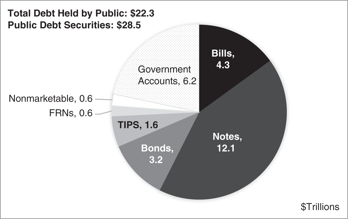
FIGURE 0.5 US Treasury Obligations, Amounts Outstanding, as of June 2021.
Source: US Treasury Bulletin.
Treasury Inflation Protected Securities (TIPS) protect investors against inflation with principal amounts that increase or decrease with changes in the consumer price index (CPI). Consider, for example, a TIPS with a principal amount of $100 and a coupon rate of 1% per year. If CPI has increased by 10%, the principal amount of the TIPS will have increased to $110, and the investor earns 1% on that higher principal amount. This investor is just as well off having $100 and earning $1 per year at the original price level as having $110 and earning 1%![]() $110 or $1.10 per year at a price level that is 10% higher. Hence, TIPS earn a fixed real or inflation‐adjusted return, while coupon‐bearing Treasuries earn a fixed nominal or dollar return.2 For this reason, by the way, in discussions that include both TIPS and Treasury bonds, the latter are often referred to as nominal bonds. In any case, while comprising only 5.6% of the total in Figure 0.5, TIPS have an outsized importance as measuring the market's perception of inflation and the price of inflation risk. As of January 2022, for example, the rate on five‐year nominal Treasury bonds was about 2.8% higher than the rate on five‐year TIPS. Roughly expressed, therefore, the market expects an average inflation rate of 2.8% over the subsequent five years. More precisely expressed, given inflation expectations and risk preferences, investors require a premium of 2.8% to buy five‐year nominal bonds and to assume inflation risk over that horizon.
$110 or $1.10 per year at a price level that is 10% higher. Hence, TIPS earn a fixed real or inflation‐adjusted return, while coupon‐bearing Treasuries earn a fixed nominal or dollar return.2 For this reason, by the way, in discussions that include both TIPS and Treasury bonds, the latter are often referred to as nominal bonds. In any case, while comprising only 5.6% of the total in Figure 0.5, TIPS have an outsized importance as measuring the market's perception of inflation and the price of inflation risk. As of January 2022, for example, the rate on five‐year nominal Treasury bonds was about 2.8% higher than the rate on five‐year TIPS. Roughly expressed, therefore, the market expects an average inflation rate of 2.8% over the subsequent five years. More precisely expressed, given inflation expectations and risk preferences, investors require a premium of 2.8% to buy five‐year nominal bonds and to assume inflation risk over that horizon.
Figure 0.5 next lists floating‐rate notes (FRNs). These are relatively new, having been first issued in January 2014. FRNs are sold with two years to maturity, and they pay a variable rate of interest equal to the going rate on 13‐week T‐bills plus a fixed spread. This spread entices some investors, who might otherwise roll investments of short‐term T‐bills, to sacrifice some liquidity and buy two‐year FRNs instead. From the perspective of the Treasury, FRNs lock in funding for two years, but at a cost only slightly above that of short‐term bills.3 In fact, over 2021, FRNs were sold at a spread of less than five basis points.4 In addition, somewhat cynically, FRNs seem to cost less than two‐year notes, because government accounting of interest rate cost does not penalize the risk of rates increasing in the future. In any case, the issuance of FRNs has remained limited, comprising about 2% of the total in Figure 0.5.
US Treasury issues are among the most actively traded securities in the world. This is due, in good part, to the significant role of the US dollar in international markets and to the perception of US government debt as among the best stores of value available. An additional explanation, however, is the careful management of Treasury debt issuance. More specifically, the US Treasury sets a regular auction schedule that lets investors know, in advance, which securities will be sold when and in what quantities. Furthermore, the Treasury has gradually modulated this schedule over many years to suit both the borrowing needs of the government and changing market conditions. To appreciate these points, Table 0.2 describes the auction schedule as of January 2022.
“Issue frequency” describes how often new securities of each type are issued. The Treasury has settled, for example, on issuing new notes with two, three, five, and seven years to maturity every month, while issuing new 10‐year notes, along with new 20‐ and 30‐year bonds, every quarter. Both the set of issues and their frequency have changed over time, however. For example, issuance of the 20‐year bond was eliminated in 1986 and brought back in May 2020, while issuance of 30‐year bonds was stopped after August 2001 and resumed in February 2006. And in 2000, the US Treasury introduced the concept of reopenings, which means auctioning or selling more of an existing issue. For example, Table 0.2 reports that 10‐year notes are issued quarterly and reopened monthly. In August 2021, the Treasury sold about $59 billion of a new 1.25% 10‐year note, that is, a note that had not been issued before, that pays interest on principal at an annual rate of 1.25%, and that matures on August 15, 2031. The following month, in September 2021, the Treasury sold another $42 billion of that same issue, that is, more notes with a coupon of 1.25% that mature on August 15, 2031. And again the next month, in October 2021, the Treasury sold another $41 billion of that same issue. In November 2021, however, a quarter after the first issuance of the 1.25% 10‐year notes, the Treasury sold $62 billion of a new 10‐year note, with a coupon of 1.365% and a maturity date of November 15, 2031.
TABLE 0.2 US Treasury Auction Schedule, as of January 2022.
| Security | Issue Frequency | Reopenings |
|---|---|---|
| 4‐, 8‐, 13‐, and 26‐week bills | Weekly | |
| 52‐week bills | Every 4 weeks | |
| 2‐, 3‐, 5‐, and 7‐year notes | Monthly | |
| 10‐, 20‐ and 30‐year notes/bonds | Quarterly | Monthly |
| 5‐year TIPS | Semiannually | 2 months after issuance |
| 10‐year TIPS | Semiannually | Every 2 months |
| 30‐year TIPS | Annually | Semiannually |
| 2‐year FRNs | Quarterly | Monthly |
TIPS: Treasury Inflation Protected Securities; FRNs: Floating Rate Notes.
Source: US Department of the Treasury.
One result of the auction schedule is that the most recently issued bonds of each type and maturity tend to be the ones most actively traded. In the previous example, as of November 15, 2021, the just‐issued 1.365% notes maturing on November 15, 2031, are called the 10‐year on‐the‐run notes and are likely to become the most actively traded of notes with approximately 10 years to maturity. The 1.25% notes maturing on August 15, 2031, which had been the 10‐year on‐the‐run notes, become the old notes, and over time, as even newer 10‐year notes are issued, become the double‐old notes, the triple‐old notes, etc.
Returning to Figure 0.5, nonmarketable securities is another small category of Treasury issuance. Included in this category are about $140 billion of savings bonds, which are discount securities sold directly to individual investors, and about $120 billion of State and Local Government Series bonds, commonly known as SLUGs, which are mentioned later in the context of municipal bonds.
The final category in Figure 0.5 refers to Treasury bonds sold into government accounts. These bonds are also nonmarketable and represent debt that the US government owes itself. The social security trust funds, for example, at the end of 2020, held about $3 trillion in Treasury bonds. Most people argue that these bonds do not represent any additional Treasury indebtedness, or, in other words, that there is no difference between social security benefits being paid by the Treasury directly or being paid indirectly through the payment of interest and principal on bonds in the social security trust funds. By this logic, Treasury bonds held in government accounts are excluded from most descriptions of government indebtedness. More specifically, in terms of Figure 0.5, US government debt is usually equated to “Total Debt Held by the Public,” or $22.3 trillion, rather than to “Public Debt Securities,” which adds the $6.2 trillion held in government accounts, for a grand total of $28.5 trillion.
In discussing the magnitude of government debt, and in comparing government indebtedness across countries, debt held by the public is usually normalized by gross domestic product (GDP), which measures the value of the goods and services produced in a country in a single year. The idea here is that countries with greater GDPs can safely carry greater levels of debt. With US GDP at about $22 trillion as of June 2021, the ratio of debt to GDP in the United States is about 100%, which is extremely high by historical standards. The ratio was over 100% during World War II; subsequently declined to between 20% and 50%; climbed to about 80% in the aftermath of the financial crisis of 2007–2009; and then shot up to above 100% in the wake of the COVID pandemic and economic shutdowns. For comparison purposes, the ratio of debt to GDP in Japan is currently over 230%; in Greece about 175%; in France about 100%; in the United Kingdom about 85%; in Germany and China, less than 60%; and in Switzerland, less than 40%.
Despite the historically high ratio of US debt to GDP, foreign investors continue to find US Treasuries attractive and hold a large fraction of the amount outstanding. As of June 2021, investors outside the United States held $7.2 trillion Treasuries, or 33% of the $21.8 trillion marketable securities shown in Figure 0.5. These holdings include $1.28 trillion (5.9%) in Japan, $1.06 trillion in China (4.9%), and $0.53 trillion (2.4%) in the United Kingdom.
Municipal Securities
The $4 trillion municipal securities market includes more than 50,000 issuers and approximately one million individual bond issues. Municipal bonds, sometimes called municipals or simply munis, are issued by states and local governments to fund their expenditures. Unlike most fixed income markets, the muni market is dominated by retail investors: as of June 2021, over 70% of principal outstanding was held directly by individuals, or indirectly by individuals through mutual funds and other investment vehicles.
Interest payments from munis are exempt from federal tax so long as funds raised from selling those munis are used for public projects. Therefore, investors who pay federal taxes are willing to accept lower rates of interest from munis than they would from bonds whose interest is taxed at the federal level, like corporates and Treasuries, controlling, of course, for differences in credit quality. And municipal issuers can raise funds at rates below what they would otherwise have to pay. The story is somewhat more complicated, however, because capital gains on price appreciation from munis is not exempt from federal tax. To avoid this tax, however, the market has evolved to minimize the proportion of return in the form of (taxed) price appreciation rather than (untaxed) interest. More specifically, most munis – in the current low‐rate environment – are issued at a coupon rate of 5% and, consequently, at a premium to par, that is, at a price greater than face amount. In this way, these munis are unlikely to trade at a discount and thus subject subsequent buy‐and‐hold purchasers to taxes on capital gains. With respect to state taxes, the treatment of municipal interest varies by state. Most states tax bonds issued in other states and exempt their own bonds, while some states tax both their own and other states' bonds. Washington, D.C., does not tax any municipal bond interest, and Utah exempts municipals issued in states that exempt Utah's bonds! Utah's exemption is more significant than it may seem, because states with no income tax automatically qualify. The final piece of the tax story is that about $500 billion of municipals do not qualify for the federal tax exemption, because their proceeds are used for working capital, for funding private business development, or for refinancing existing debt through particular kinds of transactions.5 These taxable munis pay interest at rates comparable to those in the corporate and Treasury markets, again controlling for differences in credit quality.
Muni bonds can be divided into three broad groups. General obligation (GO) bonds, which constitute about 25% of the market, are backed by the taxing power of the issuing municipality. Revenue bonds, which constitute about two thirds of the market, are backed by revenues from particular projects, like tolls from a bridge or highway. And within revenue bonds is a $600 billion subset of industrial revenue bonds, through which municipalities issue (tax‐exempt) debt to raise funds for private enterprises engaged in qualifying projects. The third group consists of prerefunded or defeased bonds. A muni in this category has been canceled as a municipal liability by the setting aside of sufficient cash and Treasury securities to fund all of its remaining payment obligations. These prerefunded or defeased bonds continue to exist and trade, but with their credit risk improved to that of Treasuries.6
Default rates on municipal securities have been very low. From 1970 to 2020, Moody's reports a five‐year cumulative default rate for the sector of 0.08%, which is much lower than the equivalent for corporate bonds, as discussed in Chapter 14. Nevertheless, credit risk is an important consideration for investors in the muni market, with underfunded pension obligations a particularly significant and perennial cause for concern. Historically, GO bonds, which are backed by the issuer's taxing power, were perceived as safer than revenue bonds, which are backed by particular sources of revenue that could diminish or disappear over time. This perception changed significantly, however, with the bankruptcy of Detroit in the summer of 2013. The settlement provisions that emerged in November 2014 were a combination of law, political forces, and negotiations across many interested parties. The results can be roughly summarized as follows. First, while a court ruled that state laws protecting pension benefits were trumped by federal bankruptcy law, Detroit pensions recovered over 95% of their value, although cost of living adjustments were reduced or eliminated. Health and life insurance benefits, however, recovered only 10% of value. Second, holders of water and sewer bonds, which had strong legal claims to the associated revenue streams, suffered no loss of principal. Third, GO bonds suffered significant losses, depending on their exact provisions. Unlimited tax bonds carry a pledge by issuers to raise taxes, if necessary, to pay bondholders. The unlimited tax bonds involved in the Detroit bankruptcy were, in addition, backed by specific, segregated, and voter‐approved tax receipts. Nevertheless, these bonds recovered only 74% of principal, and this negotiated, less‐than‐full recovery was attributed to the dwindling of their dedicated tax receipts due to deteriorating economic conditions in Detroit. Worse off, however, were Detroit's limited tax GO bonds, which had neither a pledge of unlimited tax increases nor dedicated tax receipts. They recovered only 34% of principal. The revelation that GO bonds can be treated like unsecured claims changed credit analysis and pricing in the muni market.
Before the financial crisis of 2007–2009, a majority of muni bonds were insured against default, for a fee, of course, by private insurers. In fact, most of Detroit's GO bonds were insured, which meant that insurers, rather than investors, suffered the losses described in the previous paragraph. In any case, muni insurers suffered massive losses during the financial crisis, not from their muni businesses, but from having insured mortgage‐related products. The ensuing damage to the industry ultimately resulted in less than 5% of new muni issues being insured. More recently, perhaps in part due to the Detroit bankruptcy, and perhaps in part due to the COVID pandemic and shutdowns, there has been a resurgence of muni insurance, rising to perhaps 10% of new issues.7
Other US Markets
Mortgages. The second largest sector in Figure 0.4 contains mortgages, at $17.3 trillion. Mortgage loans are used to purchase properties and are collateralized by those same properties. Mortgage balances finance the purchase of one‐ to four‐family residences (70%); commercial property (18%); multi‐family residences (10%); and farms (2%). A remarkable feature about the US mortgage market is that only about 45% of mortgage loan balances are held by the original lenders. The remaining 55% of balances are securitized, that is, sold by the original lenders; packaged into securities; and then sold to investors. Chapter 15 describes this market in much greater detail.8
Corporate and Foreign Bonds. The third largest sector in Figure 0.4 comprises corporate and foreign bonds, at $14.7 trillion, which includes bonds sold by US nonfinancial corporations (45%); by US financial corporations (31%); and by foreign corporations to US investors (24%), all to raise money to fund their operations and corporate transactions. Chapter 14 describes this market in detail.
Loans and Advances. Continuing counterclockwise in Figure 0.4, a little less than half of the $9.0 trillion of Loans and Advances are made by banks, and the rest by an assortment of nonfinancial and financial entities. An important feature of this sector is the securitization and trading of bank loans, which is described in Chapter 14. Consumer credit, at $4 trillion, is discussed in the next section, in the context of household balance sheets.
Agency/GSE Debt. The penultimate category of instruments in Figure 0.4 includes “agencies” or “agency bonds,” which are issued by government agencies and GSEs. These entities span a range of associations with the federal government, and their debt issues enjoy varying levels of support from the federal government. At one extreme are the Federal Housing Administration (FHA), the Small Business Administration (SBA), and the Government National Mortgage Association (GNMA). These agencies are part of the government, and their debt issues are backed by the “full faith and credit” of the United States. Moving from the full‐faith‐and‐credit framework, the Tennessee Valley Authority (TVA), which provides electricity for local power companies in Tennessee and surrounding states, is considered a federal agency. Formally, however, it is a corporation that is wholly owned by the US government, and its debt is backed by its own revenues, not – at least explicitly – by the federal government. Further away from full‐faith‐and‐credit are the Federal National Mortgage Association (FNMA) and the Federal Home Loan Mortgage Corporation (FHLMC). They are known as GSEs, but are owned by private shareholders and, having failed during the financial crisis of 2007–2009, are now under government conservatorship. Leading up to the crisis, their debt was not explicitly backed by the government, but the market expectations for full government support of their bonds was fully realized during and after the crisis. These two entities are discussed in great detail in Chapter 15.
Commercial Paper. The final category in Figure 0.4 is Commercial Paper (CP), through which the most highly rated corporations borrow short‐term funds from the public. CP is discussed further in Chapter 14.
0.3 US MARKET PARTICIPANTS
This section describes sectors of market participants. The volumes of debt securities and loans that appear as assets on the financial balance sheets of various sectors are shown in Figure 0.6, while the volumes that appear as liabilities are shown in Figure 0.7. Households, nonfinancial business, and general government (i.e., federal and municipal) hold a combined $10.0 trillion of debt securities and loans for their own savings or cash management purposes. Banks, various fund vehicles, insurance companies, pension funds, and other financial entities hold debt securities and loans as intermediaries, investing and managing funds for the ultimate benefit of others. The Monetary Authority, that is, the Federal Reserve, holds assets in the implementation of monetary policy. And the rest of the world, or foreign entities, invest $14.0 trillion in US debt securities and loans on their own or as intermediaries. On the liability side, the federal government borrows $24.3 trillion, and municipalities borrow $3.2 trillion to finance government expenses that are not covered by taxes and fees. Households borrow $17.3 trillion mostly to finance consumption, and nonfinancial businesses borrow $18.0 trillion to finance investments and acquisitions. The remaining financial sectors borrow as intermediaries, using funds borrowed from some sectors to lend or invest elsewhere. And finally, the rest of the world borrows $4.9 trillion through US debt securities and loans. The text now discusses several of these sectors in greater detail.

FIGURE 0.6 Financial Assets of Various Sectors, as of June 2021. ETF: Exchange‐Traded Fund; MMF: Money Market Fund.
Sources: Financial Accounts of the United States, Board of Governors of the Federal Reserve System; and Author Calculations.
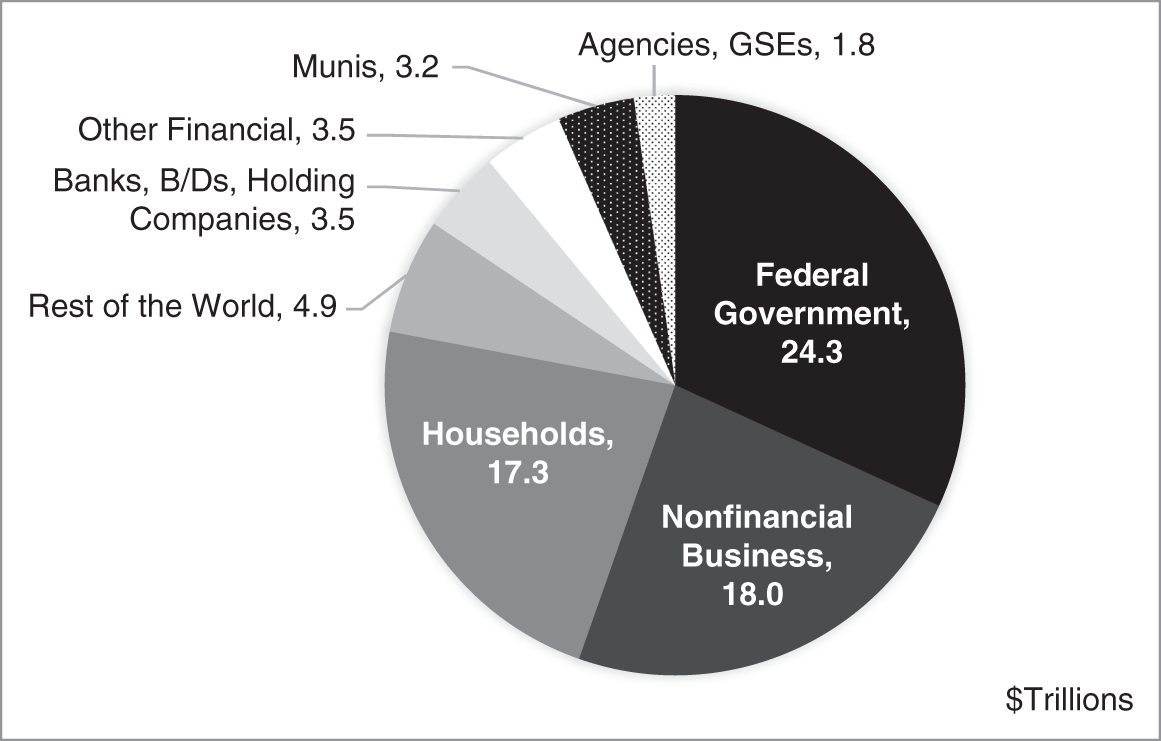
FIGURE 0.7 Financial Liabilities of Various Sectors, as of June 2021. B/D: Broker‐Dealer.
Sources: Financial Accounts of the United States, Board of Governors of the Federal Reserve System; and Author Calculations.
Households
Table 0.3 gives the financial assets and liabilities of the household sector.9 The financial assets of the sector far exceed its financial liabilities, meaning that the sector, as a whole, has significant net worth. The sector invests significant amounts directly in equity and debt markets, although a greater fraction of assets is invested through intermediaries, like pensions, mutual funds, and the savings components of life insurance policies. A large fraction of financial assets is also held in near cash equivalents, that is, in deposits and shares of money market funds. On the liability side, households borrow mostly through mortgages, which are the subject of Chapter 15, or through consumer credit.
TABLE 0.3 Financial Assets and Liabilities of Households, as of June 2021. Amounts are in $Trillions.
| Instrument | Amount | Percent of Total |
|---|---|---|
| Total Financial Assets | 113.1 | 100 |
| Pension Entitlements | 31.0 | 27.4 |
| Corporate Equities | 30.5 | 26.9 |
| Deposits and MMFs | 17.1 | 15.1 |
| Equity in Noncorporate Business | 13.7 | 12.1 |
| Mutual Funds | 12.3 | 10.9 |
| Debt Securities and Loans | 5.1 | 4.5 |
| Life Insurance Reserves | 1.9 | 1.7 |
| Other | 1.7 | 1.5 |
| Total Liabilities | 17.7 | 100 |
| Home Mortgages | 11.3 | 63.8 |
| Consumer Credit | 4.3 | 24.1 |
| Other | 2.1 | 12.1 |
Sources: Financial Accounts of the United States, Board of Governors of the Federal Reserve System; and Author Calculations.
The primary components of consumer credit are home equity loans, auto loans, credit card loans, and student loans. The outstanding credit balances of these sectors over time are depicted in Figure 0.8. Home equity loan balances grew rapidly with the run‐up of housing prices preceding the financial crisis of 2007–2009 and have declined steadily since.10 Credit card loans also grew going into the crisis, though not as dramatically, and also declined after the crisis, but had then recovered, until declining again with the COVID pandemic and shutdowns. Auto loans, while also declining through the crisis, seemingly emerged as taking the place of declining home equity loans and relatively flat credit card loans. Student loans have increased independently of the economic cycle, which is a policy result: the federal government has been guaranteeing student loans for decades and, since 2010, directly owns all of its student loans. As of March 2021, government student loan balances comprised over 92% of the total.11
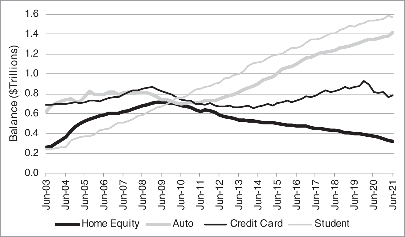
FIGURE 0.8 Balances of Consumer Credit Sectors.
Source: Quarterly Report on Household Debt and Credit, Federal Reserve Bank of New York.
Figure 0.9 reports balances that are 90 or more days delinquent, that is, balances on which the borrower has not made payments for 90 or more days. Not surprisingly, home equity delinquencies increased during and for several years after the financial crisis, as falling housing prices made it impossible for many homeowners to recover their outstanding mortgage and loan balances by selling their homes. Home equity delinquencies have since steadily declined, perhaps reflecting more careful underwriting in the aftermath of the crisis. Credit card delinquencies also increased after the crisis, perhaps reflecting weakened consumer balance sheets, but have since declined to pre‐crisis levels. Auto loan delinquencies increased after the crisis as well, then fell, and increased again, perhaps an expected consequence of the rapid growth in balances. Student loan delinquencies have been increasing for many years, which has raised a number of policy concerns, from the perspective of both students and the federal government. Note that the precipitous decline in student loan delinquencies in the second half of 2020 is an artifact of federal COVID forbearance programs.
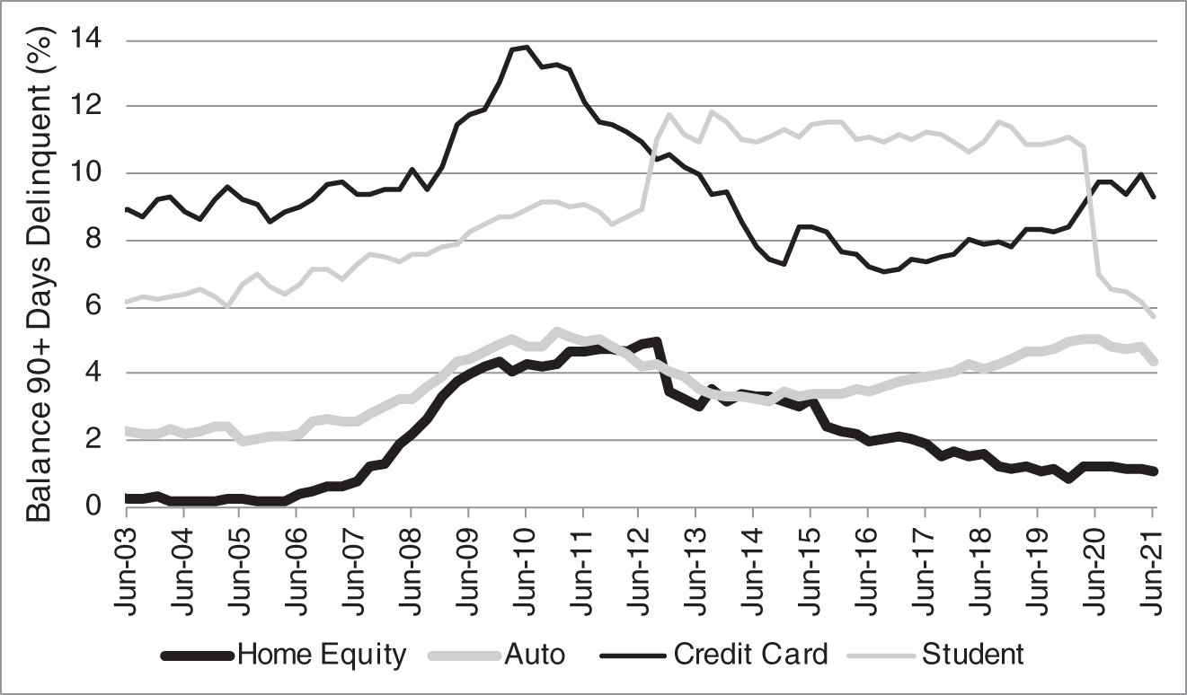
FIGURE 0.9 Delinquencies in Consumer Credit Sectors.
Source: Quarterly Report on Household Debt and Credit, Federal Reserve Bank of New York.
Nonfinancial Business
Figure 0.10 shows the composition of liabilities for nonfinancial businesses, separated into corporate businesses, which are likely to be relatively large, and noncorporate businesses, which are likely to be relatively small. Corporate businesses, which are more likely to have track records of earnings and established creditworthiness, have broader access to markets. They can sell debt securities to raise 30% of their financial liabilities, while noncorporate businesses sell essentially none. The “Other” source for corporate businesses includes direct investment from abroad, which is not at all a part of small business liabilities. Noncorporate businesses, then, rely mostly on mortgages, for which they need only unencumbered property. The differences in the liability structures of these two groups reflect the life cycle of business borrowings, from “family and friends,” to bank loans, to investor groups, to private placements of debt, and finally – for the largest and most established companies – to public debt securities. Chapter 14 discusses private placements and public debt issues in more detail.
Commercial Banks
Commercial banks accept deposits from their customers, pay them interest, and offer them safety – in part through federal deposit insurance – and immediacy or liquidity, that is, the ability to withdraw funds whenever necessary. Deposits, which are not classified as debt securities or as loans, are not included in Figure 0.7, but constituted 93% of commercial bank liabilities. Other liabilities include investments by the bank's parent company, long‐term debt, commercial paper, assorted loans, and repurchase agreements, or repo, which are loans collateralized by debt securities, as discussed in Chapter 10.
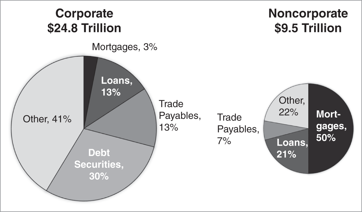
FIGURE 0.10 Nonfinancial Business Liabilities, Corporate and Noncorporate, as of June 2021.
Source: Financial Accounts of the United States, Board of Governors of the Federal Reserve System.
While deposits are certainly the main source of funding for bank investments, they are actually a product or output of banking, just like business loans and mortgages are bank products. Depositors value the safety and immediacy of deposits, and they incorporate deposits into their management of cash and liquidity. Furthermore, banks actively manage the liquidity they offer to depositors, in part by having some fraction of liabilities in longer‐term debt, and in part by investing some fraction of assets in liquid products that can be sold quickly and easily to meet any unexpected withdrawals of deposits.
Turning to assets, Figure 0.11 shows the asset composition of large and small commercial banks. Commercial and industrial (C&I) loans, real estate loans, and consumer loans are all considered the main business of banking. In addition to these assets, however, along the lines of the previous paragraph, banks hold liquid assets. The most liquid, of course, are cash, reserves or deposits at the Federal Reserve, and other money market (MM) instruments. But these assets have the disadvantage of earning very low rates of return. Therefore, to earn higher rates of return while maintaining satisfactory liquidity profiles, banks also hold Treasuries, agency securities, and MBS, which can be sold relatively easily should the need arise.
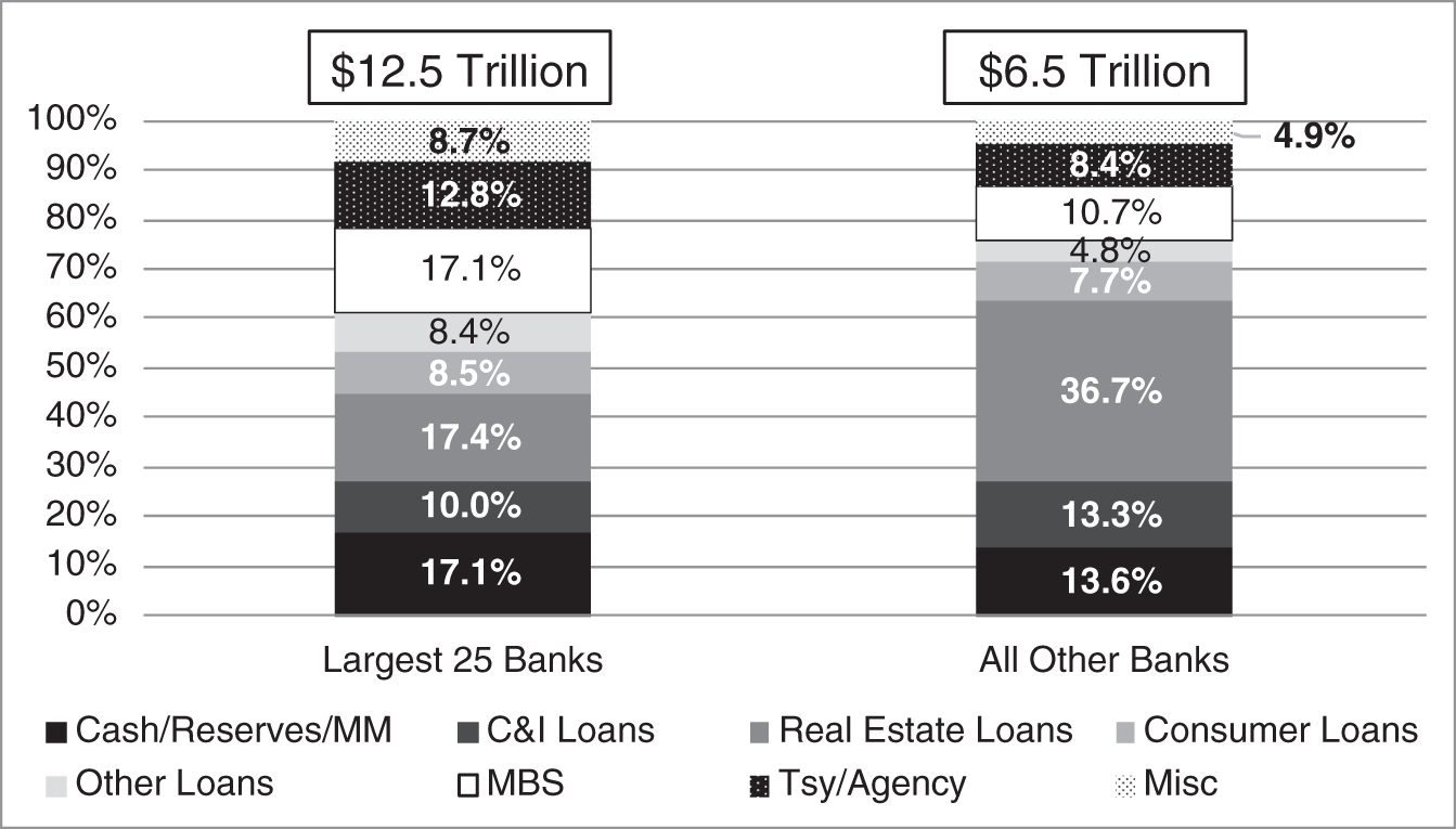
FIGURE 0.11 Assets of Commercial Banks, Largest 25 Banks and All Other Banks, as of June 2021.
Source: Assets and Liabilities of Commercial Banks in the United States, Board of Governors of the Federal Reserve System.
Figure 0.11 also reveals some differences between large and small banks. First, commercial bank assets are highly concentrated. There are over 4,000 commercial banks in the United States, but $12.5 trillion of the sector's $19 trillion of assets, or 66%, are held by the largest 25 banks.12 As an aside, the number of banks in the country has been declining gradually but swiftly: there were over 14,000 banks in 1984. This decline is likely an adjustment from historical restrictions on interstate banking and branching that prevented larger banks from satisfying market demand. In any case, a second difference between the largest and smaller banks is the difference in the fractions of their assets in real estate loans: 17.4% for the largest banks and 36.7% for the smaller banks. The concentration of a small bank's assets in real estate loans, which are often local, can challenge the bank's viability through regional economic downturns.
Life Insurance Companies
Life insurance products often pay death benefits, of course, but they are also often savings vehicles, through which policy holders invest funds with the advantages of tax deferral. Life insurance companies are, therefore, financial intermediaries that collect and invest premiums so as to meet their obligations under policies sold and to earn additional returns for their shareholders. Furthermore, long‐term fixed income assets are natural hedges to the long‐term nature of their policy liabilities. Reflecting these considerations, the asset portfolios of life insurance companies contain large fractions of corporate bonds and equities, 36.4% and 8.5%, respectively, with an additional 18.8% in mutual fund shares that are some mix of bonds and equities. In fact, their corporate bond investments make life insurers very significant players in that market: their direct holdings of $3.5 trillion of corporate bonds comprise about 24% of the total $14.7 trillion outstanding. While Treasuries are theoretically useful as a match for long‐term liabilities, they do not earn enough to meet insurer return hurdles. As a result, Treasuries comprise only 2.4% of life insurance company assets. Finally, life insurance companies also use derivatives to achieve their return and hedging objectives.
Pension Funds
Historically, the majority of pensions were defined benefit (DB) plans, in which the sponsor promises to pay retirees according to a formula that depends on the number of years worked, contributions to the plan, salary history, etc. Sponsors collect employee and their own contributions into a pension fund, and then invest the assets of that fund so as to be able to honor promised obligations. A low‐risk strategy combines relatively high contributions to the pension fund with low‐risk investments, while a high‐risk strategy combines relatively low contributions with aggressive investments. In any case, investment risk in DB plans resides with the sponsor, which, in the end, is responsible for paying the promised benefits. For decades now, however, defined contribution (DC) plans have become more important. In these plans, employees and employers contribute to individual employee accounts, and each employee can typically choose among a few investment options. Upon retirement, employee benefits are determined completely by the funds accumulated in their respective accounts. Hence, in DC plans, investment risk resides with employees. Employers can, of course, offer both types of plans or a hybrid of the two types.
Government employees, at the federal, state, and local levels, nearly always have DB plans or an option to participate in a DB plan. In the private sector, however, the trend has been for corporations and other employers to avoid the risks and costs of managing pension funds, that is, to migrate from DB to DC plans. In 1975, there were about 33.0 million participants in private DB plans and 11.5 million in private DC plans. In 2019, the numbers were 32.8 million and 109.1 million, respectively.13 Furthermore, corporations are actively shedding DB pension fund risk through pension risk transfer transactions, in which they pay insurance companies to assume their pension liabilities. In any case, for any portfolio manager of a DB plan, long‐term debt instruments naturally hedge the present value of fixed liabilities. On the other hand, allocations to equities hold out the prospect of having to make smaller contributions to the fund. A study of the largest 100 DB plans offered by US public companies in 2020 found that 50% of assets were invested in fixed income, 32% in equity, and 18% in other categories (e.g., real estate, private equity, hedge funds).14
Money Market Funds
As mentioned earlier, in the context of deposits, there exists significant demand for assets that provide both safety and immediacy. Money market funds, created in the 1970s, were designed to offer safety and immediacy, while paying higher rates than banks at the time were allowed to pay on deposits. Money market funds are divided into three broad categories: government funds, which purchase only short‐term, government‐backed debt; prime funds, which invest predominantly in short‐term, high‐quality corporate debt, like commercial paper; and tax‐exempt funds, which invest in short‐term, high‐quality, tax‐exempt municipal debt. Before changes implemented after the financial crisis of 2007–2009, investors could buy money market fund shares for $1 per share; their money was invested in relatively safe and liquid assets; and, except in extraordinary circumstances, they could sell their shares at any time for $1 per share. More specifically, a fund that i) complied with Securities and Exchange Commission (SEC) rules governing the safety and liquidity of fund investments, known as 2a‐7 rules; and ii) had a portfolio or net asset value (NAV) corresponding to a value per share of between 99.5 cents and $1.005, could offer and redeem shares at a “fixed NAV” or “stable NAV” of $1 per share. But if the value of the fund fell such that the value per share fell below 99.5 cents, the fund would “break the buck” and shares would no longer be redeemed at $1, but rather at a value corresponding to the fund's NAV. Hence, money market fund shares were very similar to bank deposits, but did not have the benefit of an explicit government guarantee, like federal deposit insurance. Instead, money market shareholders had to rely on their fund sponsors or management companies to make up for any NAV shortfalls. Only one money market fund had ever broken the buck, in 1994, but it was to happen a second time during the financial crisis of 2007–2009.
In September 2008, a few days after the failure of the mortgage government‐sponsored enterprises, FNMA and FHLMC, and a few days before the failures of the investment bank, Lehman Brothers, and the insurer, AIG, money market fund investors embarked on a flight‐to‐safety, through which they withdrew huge volumes of cash from prime funds and deposited huge volumes into government funds. Relatively suddenly, investors came to believe that financial entities might not be able to pay off their maturing commercial paper, which comprised a significant part of prime money market fund portfolios. And, in fact, the day after the bankruptcy of Lehman Brothers, the Reserve Primary Fund became the second fund in history to break the buck: the value of its sizable holdings of Lehman Brothers commercial paper had fallen so precipitously that the fund's NAV fell to 97 cents per share.15 Fearing that investor flight from prime money market funds would exacerbate already stressed conditions in money markets, including the ability of financial entities to continue borrowing in CP markets, the Treasury instituted a program through which it guaranteed money market fund shares for one year, and the Federal Reserve created a facility that extended nonrecourse loans to banks collateralized by asset‐backed commercial paper bought from money market funds.
After the crisis, the SEC changed several rules governing money market funds.16 First, 2a‐7 rules were tightened to increase the safety and improve the liquidity profiles of money market fund portfolios. Second, institutional prime and tax‐exempt money market funds, as opposed to funds with only retail investors, must allow share price to float with the fund's NAV. Proponents of this change argue that floating NAVs raise awareness that fund values can fluctuate and may discourage withdrawals timed to precede a fund's breaking the buck. Opponents argue that money market fund investors, particularly institutional investors, are well aware of the risks; that floating NAVs have little to no bearing on flights‐to‐safety away from prime funds; and that floating NAVs significantly increase the accounting, operational, tax, and legal complexities of using money market funds for cash management. The third post‐crisis change was that prime and tax‐exempt money market funds had to have the power, under various stress conditions, to impose redemption fees of up to 2% and gates that prevent withdrawals for up to 10 business days in any 90‐day period. Redemption fees, which are paid into the fund, are intended both to discourage investor withdrawals in a crisis and to recover losses from liquidating assets in a crisis to meet those withdrawals. Gates are intended to give funds a grace period in which to manage through stressed market conditions. If, however, a fund cannot restore stability by the end of its grace period, the fund is liquidated. Government funds, by the way, may choose to include the power to impose fees and gates, but very few have done so. While redemption fees and gates are intended to increase fund stability, they might actually encourage earlier, preemptive redemptions. In any case, both the floating NAV rule on institutional prime funds and the inclusion of redemption fees and gates on all prime funds went into effect in October 2016.
Figure 0.12 shows the balances of money market funds over time, by sector. The timing of the steep drops in the balances of both prime and tax‐exempt funds corresponds closely to the October 2016 effective date just mentioned. The inconvenience of floating NAVs and the potential loss of immediacy from redemption fees and gates clearly reduced the attractiveness of prime funds. In 2020, as part of a broad flight‐to‐quality brought on by the COVID pandemic and economic shutdowns, balances in government money market funds increased markedly. Over the whole of 2020, institutional prime fund balances stayed relatively constant at $600 billion, while retail prime fund balances fell gradually from about $500 billion to $200 billion. Prime balances did fall dramatically, however, in March 2020, and institutional balances fell more than retail balances, but, due to swift action by the Treasury and Federal Reserve in support of financial markets in general and money market funds in particular, balances recovered relatively quickly. In any case, it seems that the possibility of redemption fees and gates in March 2020 did encourage preemptive withdrawals by prime investors and sales of assets by prime fund managers, who raised liquidity in order to avoid triggering fees and gates. Consequently, at the time of this writing, the SEC is revisiting fees and gates and considering other changes to the regulation of institutional prime funds.17
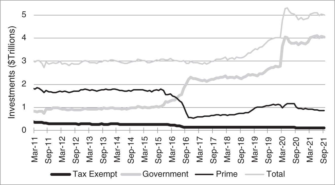
FIGURE 0.12 Balances in Money Market Funds, by Sector.
Source: US Money Market Fund Monitor, Office of Financial Research, US Department of the Treasury.
0.4 MONETARY POLICY WITH ABUNDANT RESERVES
To introduce the roles of the Federal Reserve system or “the Fed” as a modern central bank, Table 0.4 shows its pre‐crisis balance sheet, as of December 2007. One role, the creation and maintenance of a widely accepted national currency, is achieved by purchasing government bonds with that currency. The currency of the United States is comprised of green bills labeled as liabilities of the Federal Reserve, that is, as “Federal Reserve Notes.” In terms of the balance sheet, therefore, outstanding currency is a liability and Treasury securities are assets. Put another way, currency is “backed” by government bonds. As shown in the table, $773.9 billion of currency outstanding was about 83% of Federal Reserve liabilities.
TABLE 0.4 Balance Sheet of the Federal Reserve Banks, December 31, 2007, in $Billions.
| Assets | Liabilities | ||
|---|---|---|---|
| Currency Outside Banks | 773.9 | ||
| Discount Window Loans | 48.6 | Bank Reserves and Vault Cash | 75.5 |
| Treasury Securities | 740.6 | Due to US Treasury | 16.4 |
| Repo | 46.5 | Repo | 44.0 |
| Other | 115.2 | Other | 25.2 |
| Total | 950.9 | Total | 935.0 |
Sources: Board of Governors of the Federal Reserve System; and Author Calculations.
A second role of the central bank is to provide liquidity to banks under short‐term distress. As mentioned earlier, bank assets, like loans, are relatively illiquid, while bank liabilities, like deposits or short‐term borrowings from other financial institutions, may be due immediately. Therefore, a bank may find itself solvent but illiquid, that is, with assets of sufficient value to pay off its liabilities but without enough cash on hand to meet its immediate obligations. In these situations, a bank can borrow from the Fed through the discount window on any acceptable collateral. The discount window borrowings of a well‐managed bank are expected to be infrequent and of relatively limited duration.
The third role discussed here, as set out in the Federal Reserve Act, is to “maintain long run growth of the monetary and credit aggregates…so as to promote effectively the goals of maximum employment, stable prices, and moderate long‐term interest rates.” Despite the three objectives, by the way, the Fed is often said to have a “dual mandate” of full employment and low inflation. In any case, two points are made before proceeding:
- To ensure that banks have the resources to honor all requests to withdraw deposits that they are likely to receive, banks have been required to maintain cash and reserves, which are deposits held at a Federal Reserve bank. Until 2008, banks did not earn interest on their reserve balances.18
- The Fed sets the total amount of reserves in the banking system. To add to reserves, the Fed might buy a Treasury bond from a bank. The bank's account at its Federal Reserve Bank is credited with the purchase price – which increases bank reserves and the liabilities of the Fed – and the Treasury bond is added to the assets of the Fed. The Fed can also add to reserves by lending money to a bank through a repurchase agreement or repo.19 The money is credited to the bank's account at the Fed, which is a reserve liability of the Fed, and the loan obligation is added to the Fed's assets. To reduce reserves, the Fed can do the opposite of these two transactions, that is, sell a bond to a bank or borrow money from a bank through a repo. In light of this discussion, the quantity of Treasury assets and net repo assets on the Fed's balance sheet enter into the determination of the total amount of reserves in the banking system.
Before the financial crisis of 2007–2009, reserves were scarce in the sense that banks traded reserves among themselves in the interbank fed funds market. Banks that needed reserves to satisfy their reserve requirements borrowed fed funds, while banks that had excess reserves, on which they did not earn interest, loaned fed funds at the market‐determined fed funds rate. In this setting, if the Fed wanted to ease monetary conditions, to stimulate the economy (i.e., growth was too low and inflation not a threat), it would add reserves to the banking system, which – by increasing supply relative to demand in the market for reserves – would decrease the fed funds rate and likely increase the volume of bank loans to commercial enterprises. Similarly, if the Fed wanted to tighten monetary conditions, to slow the economy (e.g., growth was too inflationary), it would remove reserves from the system, which would increase the fed funds rate and likely decrease bank loans to commercial enterprises. Finally, the means by which the Fed changed reserves were called open market operations and consisted almost exclusively of lending and borrowing money through repurchase agreements.
In response to the financial crisis and ensuing Great Recession, the Fed tried to stimulate the economy as just described, by reducing the fed funds rate from 5.25% in September 2007 to a range of between 0% and 0.25% by December 2008. But having reduced interest rates to nearly zero and wanting to stimulate the economy even more forcefully, the Fed began what became known as quantitative easing (QE): it purchased great quantities of US Treasury securities and “agency MBS,” which are MBS issued by government agencies and GSEs. At the start of the program, purchases of MBS directly eased stresses arising from the overleveraged positions in mortgages and mortgage products that were at the heart of the crisis. Experts do not agree, however, on the mechanism by which the subsequent massive purchases of both Treasuries and MBS were to stimulate the economy, although possibilities include lowering intermediate‐ and long‐term interest rates (rather than just the fed funds rate); pushing investors out of relatively safe Treasuries and agency MBS and into riskier products like corporate bonds and loans; and flooding banks with reserves. In fact, the chairman of the Fed at the time said a few years later that “the problem with QE is that it works in practice, but it doesn't work in theory.”20
Figure 0.13 shows the composition of the asset side of the Fed's balance sheet from June 2006 to June 2021. Note that the total of Fed assets is often referred to by market participants simply as the Fed's “balance sheet.” In any case, during the financial crisis itself, from 2007 to 2009, assets were elevated by expanded repo lending, lending through the discount window, loans through emergency facilities that the Fed put in place at the time, and through swap lines, through which the Fed lends US dollars to foreign central banks, collateralized by foreign currency. While small in hindsight, this balance sheet expansion before QE was unprecedented, increasing from about $900 billion at the start of 2007 to over $2 trillion by the end of 2008. From then, the Fed fully engaged in QE by purchasing Treasuries and agency MBS, and the balance sheet grew dramatically. By the end of 2014, however, the Fed decided that economic conditions had improved enough to discontinue further stimulus. It stopped buying new assets, though it continued to roll over principal repayments from its holdings. From December 2015 to summer 2019, it raised the target Fed funds rate from a range of 0% to 0.25% to a range of 2.25% to 2.50% and, in what was named the “normalization” of the balance sheet, began allowing assets to decline with principal repayments. The Fed was clear to point out, however, that the balance sheet would not decline to anywhere near its size before the financial crisis, because, as explained later, post‐crisis monetary policy requires greater levels of reserves. Along these lines, in summer 2019, the Fed resumed the reinvestment of principal payments to maintain the size of the balance sheet. Then, in response to turmoil in the repo market in September 2019, further described later, the Fed started growing the balance sheet again. The Fed also judged that “implications of global developments for the economic outlook as well as muted inflation pressures” warranted lowering rates and reduced the Fed funds target range to 1.50% to 1.75% by November 2019. Finally, with the onset of the COVID pandemic and economic shutdowns, the Fed reduced rates back to the range of between 0% and 0.25% and aggressively bought Treasuries and MBS. As of June 2021, the Fed's balance sheet stood at $8.25 trillion, more than nine times its size before the financial crisis.
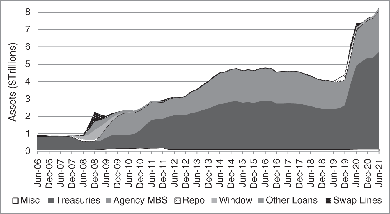
FIGURE 0.13 Assets of Federal Reserve Banks, by Instrument.
Source: Board of Governors of the Federal Reserve System.
QE not only increased the size of the Fed's balance sheet but also changed its nature in a way that necessitated a new approach to implementing monetary policy. This is best described in terms of the liability side of the balance sheet, which is shown in Figure 0.14 for three dates: the end of 2007, before the financial crisis; the end of 2019, before the pandemic; and, most recently, the end of the second quarter of 2021. At the end of 2007, consistent with the pre‐crisis implementation of monetary policy, about 2% of the Fed's liabilities were bank reserves, and reserves were scarce. After years of QE, however, with Fed asset purchases adding to bank reserves, bank reserves rose to 37% of Fed liabilities by the end of 2019 and 43% by June 2021. Reserves had become abundant, and banks essentially stopped borrowing from and lending reserves to each other.21 Consequently, in this new regime of abundant reserves, the Fed could no longer influence short‐term rates by adding to or subtracting reserves from the banking system.
The Fed currently sets interest rates through two administrative rates, the interest on reserve balances (IORB) and the reverse repo facility (RRP) rate. The IORB is the rate that the Fed pays banks on their reserve deposits. Focusing on overnight, safe rates, that is, putting aside spreads due to longer terms, riskier investments, and fees, the IORB fixes the rate at which banks are willing to borrow and lend. No bank would borrow at a rate above the IORB: it would be less costly to use reserves and sacrifice earnings at the IORB. And no bank would lend at a rate below the IORB: it would be more profitable to keep reserves on deposit and earn the IORB.22
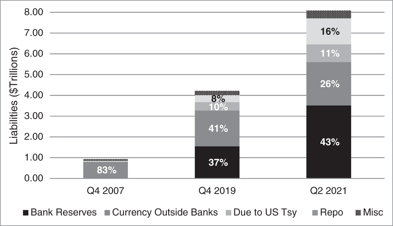
FIGURE 0.14 Liabilities of Federal Reserve Banks, by Instrument.
Source: Board of Governors of the Federal Reserve System.
If banks were the only participants in money markets, then setting the IORB would set overnight, safe rates in the system. But nonbanks with funds to lend might very well lend at rates below the IORB. First, only banks hold reserves and, therefore, only banks can lend to the Fed directly at the IORB. Second, because of post‐crisis regulations, discussed later, banks are not willing to accept deposits from all comers and then hold those funds as their own reserves at the Fed. Therefore, other significant market participants, particularly money market funds, might very well lend funds at rates below the IORB. To prevent these lenders from pushing market rates below Fed targets, the Fed offers to pay a minimum rate to these participants through its RRP. More specifically, through the RRP, money market funds and some other entities can lend money to the Fed, taking Treasury securities as collateral, at the Fed's administered RRP rate.23 It has turned out, in fact, that the facility has had to grow very large and very quickly to keep rates in the Fed's policy range. Figure 0.14 shows that, as of June 2021, the Fed's repo liabilities of $1.3 trillion constituted 16% of the Fed's total liabilities.
Putting these pieces together, the Fed sets rates in the regime of abundant reserves as follows: the Fed sets a target range for the market‐determined fed funds rate; it sets the IORB to determine the rate at which banks are willing to borrow and lend; and it sets the RRP rate as a floor to the rate at which money market funds and others will lend. At the time of this writing, the fed funds target range is between 0% and 0.25%; the RRP rate is 0.05%; and the IORB is 0.15%. This means of implementing monetary policy has been successful in that the weighted‐average of fed funds transactions has most recently been between 0.06% and 0.10%.
Policy implementation with abundant reserves has not been as successful, however, with respect to banks responding to market conditions without Fed assistance. Put another way, it has not been clear at what level reserves really are abundant. In mid‐September 2019, reserves dropped by about 9% somewhat suddenly, from a variety of causes, including corporate tax payments and the settlement of new Treasury issues, both of which move funds from banks to the government. Banks might have been expected, with their abundant reserves, to supply funds to any market participant needing funds. But that did not happen. Instead, in the ensuing scramble for funds, when the Fed's target range was between 2% and 2.25%, the transaction‐weighted repo rate on a particular day averaged 5.25%, and one trade was done at 10%. As mentioned earlier, the Fed responded swiftly by adding reserves, but the episode demonstrated that the determination of the quantity of reserves in a system of abundant reserves was not necessarily straightforward.
The reasons that reserves proved inadequate were traced to the interactions of monetary policy with bank regulation. First, since the financial crisis, banks have been subject to a leverage ratio, which requires that capital equal a minimum fraction of assets, regardless of the risk of those assets. In particular, reserves at the Fed, which are safer than any other instrument in the system, and repo lending on Treasury securities, which is extremely safe, are now both subject to capital requirements. Second, since the financial crisis, banks must hold enough high‐quality liquid assets (HQLA) to meet certain scenarios of cash withdrawals and funding needs. Furthermore, while Treasury securities can be used to meet HQLA requirements, there appears to be a bank examiner preference for reserves. Third, a stigma remains for banks that have daylight overdrafts, that is, temporary negative balances at Fed accounts that have to be resolved by the end of the day. Returning to September 2019, then, banks were not willing to make additional repo loans, despite the relatively high rates available, because the loans would increase assets and capital requirements; use reserves; and risk daylight overdrafts.24
A similar episode occurred in March 2020. News of the COVID pandemic and economic shutdowns resulted in disorder in Treasury markets, manifested through high costs of trading and high spreads between otherwise similar securities. These disturbances were much more severe than those in September 2019, but banks again seemed unwilling to use their resources, and the Fed again intervened by reducing the fed funds target range, offering unlimited repo loans, purchasing Treasuries and MBS, and temporarily excluding reserves, Treasuries, and Treasury repo from leverage ratio calculations.25 As a more permanent response to the episodes of both September 2019 and March 2020, the Fed instituted a standing repo facility (SRF) in July 2021, through which primary dealers and bank counterparties can borrow money overnight from the Fed on government‐backed collateral. To discourage the use of the facility except under stressed conditions, the borrowing rate is set above market rates. At the time of this writing, with the RRP rate at 0.05% and the IORB at 0.15%, the rate on the SRF is 0.25%.
Several policy issues arise with QE and the implementation of monetary policy in a regime of abundant reserves. First, the Fed was established and has traditionally accepted deposits only from banks. The idea was that the public deposits funds into banks, and banks decide to whom to make loans. In other words, the private banking sector was responsible for capital allocation decisions. The Fed has always held some quantity of government bonds, of course, because, in the current monetary system, as explained earlier, government bonds are the assets against which circulate the liability of central bank currency. But the purchase of much greater quantities of Treasuries – currency has fallen to only 26% of Fed liabilities – and the purchase of MBS by the Fed, are effectively capital allocation decisions. Furthermore, the acceptance by the Fed of large deposits from the public through the RRP has disintermediated banks as well. A second policy issue is that the existence of the RRP may encourage the public, in a crisis, to withdraw funds from banks and buy money market fund shares, to be deposited in the RRP. While withdrawing money from banks in cash has always been an option during crises, before the RRP this was very inconvenient for large sums. Third, to the extent that there is some limit on the size of a central bank's balance sheet, maintaining a large balance sheet in relatively normal times limits room for action in future times of stress. Fourth, the Fed is now paying banks interest on their reserves, which it was not doing before 2008. This can be viewed as a cost to taxpayers when, for example, the Treasury is borrowing through three‐month T‐bills – and the Fed is investing some of its assets in those same T‐bills – at five or six basis points, while the Fed is borrowing from banks through reserves at 15 basis points. And this issue could become more acute when the Fed eventually increases rates by increasing the IORB. In fact, one of the reasons that the Treasury has been keeping more of its cash balances or deposits at the Fed is to avoid the situation in which Treasury holds stores of cash as deposits at banks, earning a relatively low rate of interest, while the banks are depositing those fund at the Fed and earning the IORB.26 Figure 0.14 shows that Treasury deposits have grown to about 11% of Fed liabilities.
0.5 NEGATIVE RATES AND QE IN EUROPE AND JAPAN
Lending €1 at a negative rate means receiving less than €1 when the loan matures. Conversely, borrowing €1 at a negative rate means paying back less than €1 at maturity. Buying a bond at a negative yield means purchasing the bond for more than its face amount, receiving no interest over the life of the bond, and receiving only face amount at maturity.27 Individuals with relatively small amounts of money can avoid lending at negative rates by keeping money in cash. For individuals and corporations with larger sums, however, holding cash is very cumbersome, and depositing funds at a bank at a modestly negative rate of interest may be the best available choice. There are also reasons to buy long‐term bonds trading at a negative yield, despite their being guaranteed to lose money in nominal or euro terms. First, if bank deposit rates are negative, say at ![]() 0.50%, then purchasing a bond yielding −0.25% might be preferable to a deposit. Second, if the future is characterized by falling prices, that is, by deflation, then a negative yielding bond can offer a positive real return. For example, a bond yielding
0.50%, then purchasing a bond yielding −0.25% might be preferable to a deposit. Second, if the future is characterized by falling prices, that is, by deflation, then a negative yielding bond can offer a positive real return. For example, a bond yielding ![]() 1% when prices are falling at a rate of 2% is actually gaining 1% in real terms, that is, in purchasing power. Third, from a short‐term trading perspective, negative yielding bonds increase in price if yields fall. In other words, a trader makes money by buying a bond at a yield of
1% when prices are falling at a rate of 2% is actually gaining 1% in real terms, that is, in purchasing power. Third, from a short‐term trading perspective, negative yielding bonds increase in price if yields fall. In other words, a trader makes money by buying a bond at a yield of ![]() 1% if market yields subsequently fall to
1% if market yields subsequently fall to ![]() 1.5%.
1.5%.
The Fed never lowered its target interest rate below zero as part of its easing program, but the European Central Bank (ECB) combined negative rates with QE starting in 2014, and the Bank of Japan did so in 2016. These policy decisions contributed to a peak of more than $18 trillion of global debt trading at negative yields in December 2020, and nearly as much as recently as summer 2021, with more than 50% of that volume in European bonds and about a third in Japanese bonds.28 At the time of this writing, with central banks around the world expected to increase rates in response to inflation, the volume of negative yielding bonds is significantly lower, at less than $5 trillion in early 2022.
The Eurosystem refers to the ECB and the collection of national central banks in the euro area. Individual banks conduct transactions with and keep reserves at their respective national central banks, which, in turn, interact with the ECB. For simplicity, however, the discussion here is written as if banks trade directly with the ECB. The ECB targets interest rates by setting a deposit facility rate, which banks earn on their reserve deposits at the ECB, and a rate on main refinancing operations, which banks pay to borrow from the ECB through short‐term repo transactions.29 In its easing of monetary conditions, the ECB lowered these policy rates from 3.25% and 4.25%, respectively, in July 2008, to ![]() 0.50% and 0%, respectively, in September 2019. An individual bank might try to avoid earning a negative interest rate on its reserve deposits by lending out its reserves, which essentially passes them on to another bank. The banking system as a whole, however, cannot reduce the total amount of reserves supplied by the ECB and, therefore, cannot collectively avoid the negative rates on reserves. While the logic of reducing rates to stimulate economic activity can be extended to negative or even significantly negative rates, policymakers around the world have not been eager to go far along that path. Banks quickly passed negative rates on to their corporate depositors but have been reluctant or unable to do so for the vast majority of their retail depositors. Consequently, contrary to policy objectives, extended periods of negative rates seem to have reduced both bank profitability and lending activity.30
0.50% and 0%, respectively, in September 2019. An individual bank might try to avoid earning a negative interest rate on its reserve deposits by lending out its reserves, which essentially passes them on to another bank. The banking system as a whole, however, cannot reduce the total amount of reserves supplied by the ECB and, therefore, cannot collectively avoid the negative rates on reserves. While the logic of reducing rates to stimulate economic activity can be extended to negative or even significantly negative rates, policymakers around the world have not been eager to go far along that path. Banks quickly passed negative rates on to their corporate depositors but have been reluctant or unable to do so for the vast majority of their retail depositors. Consequently, contrary to policy objectives, extended periods of negative rates seem to have reduced both bank profitability and lending activity.30
To ease monetary conditions beyond reducing interest rates, the ECB turned both to loans to banks and to QE. Figure 0.15 shows the assets of the ECB or, more precisely, the consolidated assets of the ECB and the national banks in the Eurosystem. Over the whole period, the multiplicative expansion of the balance sheet was similar to that at the Fed, shown in Figure 0.13. The ECB began at a slower pace, however, and, at the start, placed a heavier reliance on bank loans. Before the financial crisis, the ECB loaned money to banks on a collateralized basis for a week through its main refinancing operations (MROs) and for three months through its longer‐term refinancing operations (LTROs). As the ECB wanted to ease monetary conditions, it offered longer‐maturity LTROs, first up to a year and then up to three years. The logic was that banks have more flexibility to expand their lending if they are more certain of their source of funds. Then, starting in 2014, with the aim of making its loans even more stimulative, the ECB began targeted long‐term refinancing operations (TLTROs), which made four‐year loans to banks in amounts based on the amounts that banks, in turn, loaned to their customers. At the time of this writing, MROs are for a week, LTROs for three months, and TLTROs for terms up to four years. As evident from Figure 0.15, however, the ECB eventually expanded its balance sheet less through loans and more through QE, that is, through the purchase of securities. While government debt issues comprise the vast majority of these purchases, the ECB began purchasing nonbank corporate obligations in early 2016, and, as of early 2022, owns more than €350 billion of these securities.31
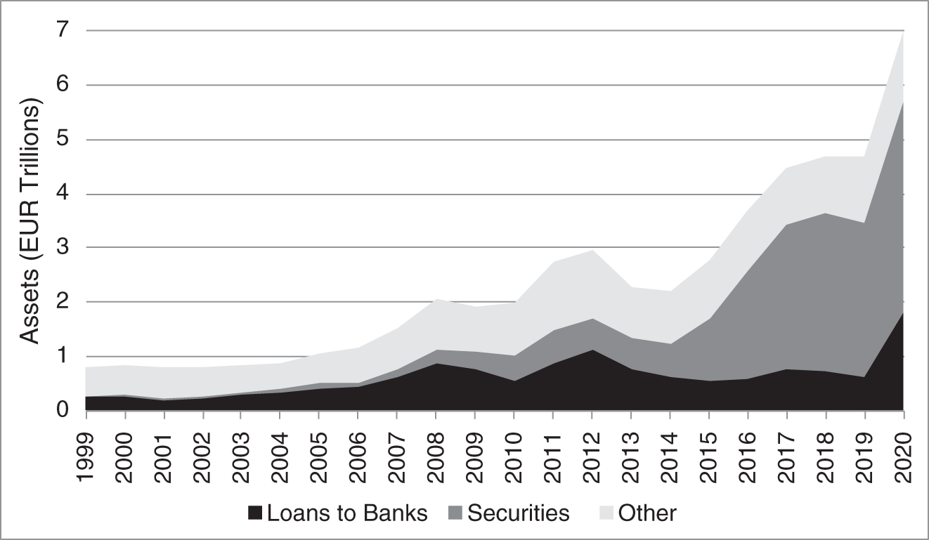
FIGURE 0.15 Consolidated Balance Sheet of the Eurosystem, Assets.
Source: European Central Bank.
The ECB faces a unique challenge in implementing QE. European law prevents the ECB from funding individual European governments, or more broadly, from encouraging any unsound budget policies. In this spirit, to preserve ECB purchases as purely monetary rather than fiscal interventions, the ECB has aimed to purchase the bonds of various national governments in proportions to their capital keys, which reflect the sizes of their populations and economies. Furthermore, in 2015, the ECB limited itself to purchasing at most one third of the outstanding amount of any country's bonds. As QE purchases grew, however, keeping within these constraints has been difficult, and the ECB faced court challenges with respect to some of its decisions. One obstacle of growing significance has been that Germany has the greatest capital key, but a relatively small amount of debt outstanding. The ECB gave itself more leeway, therefore, for purchases under the Pandemic Emergency Purchase Programme in March 2020: the one‐third limit would not be applied; the shortest eligible maturity would be 28 days rather than one year, which allowed for the purchase of short‐term German government bills; bonds with less than investment‐grade ratings would be eligible, which allowed for the purchase of Greek government debt; and some flexibility would be tolerated with respect to the capital keys constraint.32
Apart from allocating purchases across countries, the sheer magnitudes of ECB purchases have become challenging. For example, in June and July 2021, the ECB purchased €134.7 billion of government bonds from France, Germany, Italy, and Spain, while, over the same time period, the net issuance of those countries was only €89 billion. Furthermore, by the end of 2021, the ECB was expected to own more than 40% of all German and 40% of all Italian government bonds outstanding.33
One development that has made QE easier for the ECB is the relatively recent, large‐scale issuance of debt by the European Commission (EC). EC debt is an obligation of the European Union as a whole, and not the obligation of any particular country. While not unprecedented, such supranational European debt has never before been issued on the scale planned from 2020 to 2026. The EC is issuing €100 billion of SURE (Temporary Support to mitigate Unemployment Risks in an Emergency) bonds and €800 billion of NextGenerationEU bonds to finance expenditures aimed at supporting economic recovery from the COVID pandemic and economic shutdowns.34 The total of these supranational issues is a modest, but not insignificant, fraction of the roughly €12.5 trillion of European government debt outstanding in 2021. From the perspective of the ECB, the debt issues of the EC not only provide more eligible bonds for purchase, but also bonds that are not subject to the cross‐country purchase allocation constraints described earlier. EC debt purchases do face other constraints, however: at the time of this writing, the ECB can invest at most 10% of its portfolio in supranational debt and can hold no more than 50% of the debt of any one supranational issuer.
The Bank of Japan (BOJ) was the first central bank to introduce QE. Reacting to low growth and deflation, the BOJ had already, by 2001, pushed TONAR (Tokyo Overnight Average Rate), the Japanese interbank rate, to nearly zero. Looking for additional means of stimulus, the BOJ began its QE operations by purchasing Japanese government bonds (JGBs) with maturities greater than two years. Various additional lending and purchase programs were subsequently introduced, which included the purchase of corporate obligations, but, as shown in Figure 0.16, its balance sheet did not increase at anything like the trajectory pursued by the Fed and ultimately the ECB until 2013, with the BOJ's Quantitative and Qualitative Monetary Easing (QQE). This program committed not only to massive asset purchases, which were to include long‐term JGBs, corporate bonds, exchange‐traded funds, and equities, but also to lowering yields on long‐term JGBs. QQE showed some promising economic results at first, but by 2016 the BOJ took further action. First, it “went negative,” lowering the rate on some bank reserves to ![]() 0.10%. Second, it began yield curve control or yield curve targeting, in which it committed to buy (or sell) 10‐year JGBs so as to keep their yields at approximately 0%. Yield curve control was effective in that the BOJ did not have to purchase so great a volume of bonds as previously to keep rates low. In other words, the mere threat of central bank trading to keep yields at 0% is enough to keep market‐determined yields at that level. The effectiveness of this threat is manifested in Figure 0.16 as a slower increase in BOJ assets from 2016 until the outbreak of the COVID pandemic in 2020. While inflationary pressures in the United States and Europe, at the time of this writing, have pushed the Fed and ECB into more restrictive monetary postures, economic conditions and continued low inflation in Japan are keeping the BOJ committed to its expansionary policies.
0.10%. Second, it began yield curve control or yield curve targeting, in which it committed to buy (or sell) 10‐year JGBs so as to keep their yields at approximately 0%. Yield curve control was effective in that the BOJ did not have to purchase so great a volume of bonds as previously to keep rates low. In other words, the mere threat of central bank trading to keep yields at 0% is enough to keep market‐determined yields at that level. The effectiveness of this threat is manifested in Figure 0.16 as a slower increase in BOJ assets from 2016 until the outbreak of the COVID pandemic in 2020. While inflationary pressures in the United States and Europe, at the time of this writing, have pushed the Fed and ECB into more restrictive monetary postures, economic conditions and continued low inflation in Japan are keeping the BOJ committed to its expansionary policies.
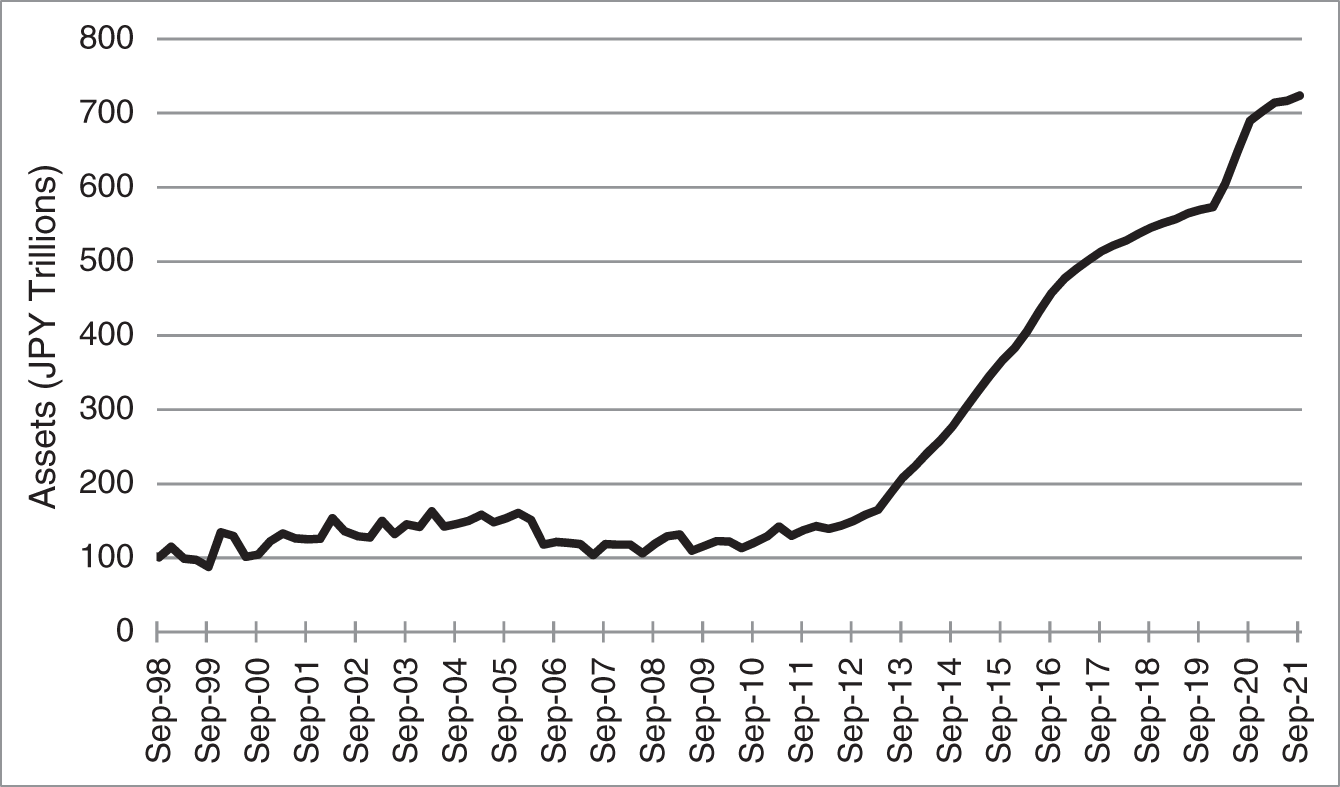
FIGURE 0.16 Assets of the Bank of Japan.
Source: Bank of Japan.
0.6 TRADING AND LIQUIDITY
An important feature of any market is liquidity, loosely defined as the extent to which a market participant can trade a desired volume of securities at close to a prevailing market price. This section begins with some definitions of liquidity and some summary statistics across fixed income markets. Several trends impacting liquidity are discussed next, including electronification; dealer regulation and risk taking; the growth of principal trading firms (PTFs); the growth of exchange‐traded funds (ETFs); and the growing concentration of asset managers. The section concludes with the implications of these trends with respect to liquidity and recent concerns about systemic fragility.
Because liquidity is hard to define precisely, there are many ways to measure it. The following are among the most common metrics:
- Bid–ask spread gives the difference between the higher ask price, at which a small amount of a security can be immediately purchased, and the lower bid price, at which a small amount of a security can be immediately sold. A market maker might expect to earn the bid–ask spread, on average, by buying securities from customers at the bid and selling to other customers at the ask. Equivalently, defining the mid price as the average of the bid and ask prices, and assuming the mid represents the fair market price, a customer can conceive of the cost of trading as half the bid–ask spread: buying at the ask instead of the mid and selling at the bid instead of the mid.
- Volume and turnover measure the amount of a security that trades over some time interval, as an absolute amount or as a percentage of the total outstanding amount of that security, respectively. A particular volume measure is average daily volume (ADV), which averages realized daily volumes over some observation period. Volume and turnover both give insight into the size of a trade being contemplated. For example, it should not be too difficult to sell $1 million face amount of a bond when its ADV is $500 million. On the other hand, it will likely be quite challenging to sell 10% of an outstanding bond issue when its daily turnover is 2%.
- Market depth is a measurement of liquidity used in connection with a central limit order book (CLOB). Through a CLOB, traders submit limit orders to buy a certain volume of a bond at a particular price (or less), or to sell a certain volume of a bond at a particular price (or more). Market depth is then defined in terms of the sum of the volumes of limit orders placed at prices from the mid to some level above or below the mid. For example, if the mid price is 100 and there are limit orders to buy $10 million face amount of bonds at prices of 99 or less, then a seller could immediately sell $10 million at 99. Unlike the bid–ask spread, therefore, market depth measures liquidity for orders of different sizes.
- Price impact or implementation shortfall. A buyer of a significant volume of a particular security can expect the market price to increase in the course of executing the purchases, as a seller of a significant volume can expect the market price to fall. Price impact measures the extent to which the market price can be expected to change as a result of a large transaction, and implementation shortfall measures the difference between the realized purchase or sale price on a large transaction relative to the market price before the transaction. Both price impact and implementation shortfall are typically estimated using data from past transactions. Asset managers and traders use the resulting models to estimate the transaction costs of their proposed trades. Dealers also use these models to quote prices at which they are willing to guarantee execution of large client orders.
The liquidity of fixed income securities varies dramatically across asset classes, across subclasses of those broader classes, and across individual securities within those subclasses. Using ADV, Table 0.5 illustrates the variation of liquidity across broad asset classes. The ADVs in the table range from over $650 billion for Treasuries and over $250 billion for agency MBS to about $9 billion for munis and even less for agency securities, asset‐backed securities, and non‐agency MBS. Variation of liquidity within these asset classes depends on the individual markets. In the Treasury market, for example, the most recently issued bonds in each maturity range are by far the most liquid (see, for example, Figure 11.1). In the corporate bond market, liquidity varies with age, credit quality, and issue size. Like Treasuries, the most recently issued corporates are the most liquid: one study reported that the monthly turnover of corporate bond issues declined from about 45% in the first month after issuance to about 13.5% in the second month and continues to decline thereafter. With respect to credit quality, investment‐grade bonds are more liquid than less creditworthy high‐yield bonds. In fact, 51.1% of the ADV of corporates in Table 0.5 is due to trading in investment‐grade bonds and only 17.5% to high‐yield bonds. (The remaining ADV is from private placements, 25.8%, and convertibles, 5.6%.) Finally, with respect to issue size, one study showed that larger issues traded on a greater number of days in a year than smaller issues. To cite a few statistics, investment‐grade bonds from issues greater than $1 billion trade, on average, on about 170 days a year. By contrast, investment‐grade bonds from issues less than $250 million trade, on average, on fewer than 20 days in a year. Note, by the way, that describing liquidity in terms of the number of days on which a particular bond trades at all indicates the illiquidity of corporate bonds, at least relative to Treasuries. As a final example, the liquidity of muni issues also declines rapidly with age. Over the whole of 2019, the volume of munis that traded within a month of their issuance was about $585 billion. But the volume of munis that traded between one and three months of their issuance was only $138 billion, and between three and six months only $77 billion, etc. Furthermore, the total 2019 trading volume of all munis that had been issued 10 or more years previously was only about $91 billion.35
TABLE 0.5 Average Daily Volumes (ADV) of Trading in Selected Markets, Fourth Quarter 2021, in $Billions.
| Market | ADV |
|---|---|
| Treasuries | 651.8 |
| Agency MBS | 251.2 |
| Corporates | 34.5 |
| Munis | 8.9 |
| Agencies | 2.4 |
| ABS | 1.3 |
| Non‐Agency MBS | 1.0 |
Source: SIFMA (2022), “SIFMA Research Quarterly – 4Q21: US Fixed Income Markets – Issuance & Trading,” January.
The text now turns to a discussion of trends affecting liquidity in fixed income markets.
Electronification
Equity and futures markets, which comprise relatively few distinct securities, migrated to electronic trading much more quickly than did bond markets, which comprise a vastly greater number of distinct issues. Traditionally, bonds were traded by voice. Customers traded with dealers, and dealers traded with each other, either directly or anonymously through interdealer brokers (IDBs). While a lot of bond trading is still by voice, electronic trading has been growing steadily. Dealer‐to‐customer (D2C) trades can take place on single‐dealer or multi‐dealer platforms, mostly through request‐for‐quotes (RFQ). In this process, a customer requests dealers to provide price quotes to trade a particular size of a particular security or portfolio of securities. The customer then chooses with which dealer to trade.36 A customer can also receive direct streams from dealers, through which dealers continuously send bid and offer prices for particular securities. The customer can then decide if and when to trade at the streamed prices. Dealer‐to‐dealer (D2D) trades can take place on interdealer electronic platforms, usually through a CLOB. Through a CLOB, traders submit limit orders to buy or sell a security, as described earlier, or they buy or sell that security immediately by lifting the offers or hitting the bids of other dealers who have submitted limit orders. PTFs have become more important in recent years and are discussed presently. PTFs often participate directly on interdealer platforms and also set up direct streams from individual dealers.
In the Treasury market, from February 2019 to May 2020, 65% of all trades were electronic. This percentage breaks up into 33% D2D trades, which nearly all trade electronically, and 67% DTC trades, of which 48% trade electronically. The electronic trades over this time period were 54% through CLOBs, 33% through RFQ, and 13% through streaming. In the corporate bond market, electronic trading of investment‐grade bonds increased from 10% in 2011, to 19% in 2017, and 31% in 2020, and reached 38% in December 2020. Lower but growing percentages of high‐yield bonds trade electronically, from 11% in 2017, to 21% in 2020, and to more than 25% in December 2020. Electronic trading of corporates is further ahead in Europe, growing from 39% of the market in 2017 to 47% in 2020.37
Dealer Regulation and Risk Taking
Dealers traditionally take risk in order to make markets. Customers can buy securities in significant size from dealers, because dealers are willing to bear the risks of buying and holding significant inventories in those securities. Customers can sell securities in significant size to dealers, because dealers are willing to bear the risks of holding and subsequently selling those securities. There are really two distinct risks here: market risk and execution risk. With respect to market risk, a dealer holding an inventory of corporate bonds can pretty easily hedge the risk of general interest rate changes, and even the risk of general changes to credit spreads, but hedging the unique credit risk of individual bonds can be difficult and expensive. With respect to execution risk, a dealer must typically “work out” of a large position. For example, after buying a large block of securities from a customer, the dealer cannot usually sell that whole block at once: the loss from the resulting price impact would likely wipe out any spread or fee that the dealer had charged the customer. Therefore, the dealer usually sells the larger position gradually, in smaller pieces, running the risk that other market participants happen to jump in to sell the same security at the same time, and also extending any idiosyncratic market risks of the position.
Dealers in banking entities were subjected to more stringent regulation after the financial crisis of 2007–2009. In particular, capital requirements were increased, both adjusted for risk and as a raw percentage of assets; liquidity requirements were formally added; and trading purely for the account of the bank, rather than for facilitating customer transactions, was – with the exception of Treasury bond trading – severely restricted by the Volcker rule. Because of this new regulatory regime, and perhaps also because of their own choices to reduce risk, banking entities are less willing to hold securities inventory and less willing to bear the risks of making markets. Figures 0.17 and 0.18 illustrate this point in the US Treasury and corporate bond markets, respectively.
Figure 0.17 shows that the amount of 10‐year Treasury notes sold at auction has been increasing steadily, and particularly rapidly in recent years, while, at the same time, dealers – who are mostly within banking entities – have been purchasing lower and lower percentages of those sales. Both the issue sizes and allotments to dealers, given in the figures by the very light gray lines, vary significantly from month to month, mostly because of the auction cycle of new and reopening sales described previously. To show the trend more clearly, therefore, the solid lines are centered seven‐month averages of the underlying series. In any case, in the last few month of the observation window, the allotment to dealers is well under 15%. Figure 0.18 shows that primary dealers are holding much smaller net positions in corporate bonds than before the crisis, while the total amount of corporate bonds outstanding has increased dramatically.38
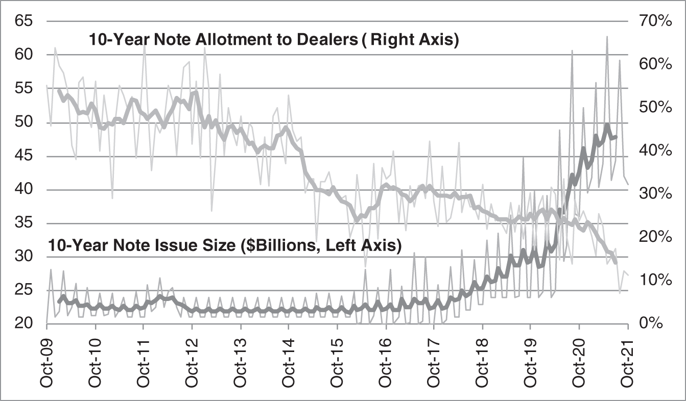
FIGURE 0.17 10‐Year Treasury Note Auction Size and Allotment to Dealers.
Sources: Investor Class Auction Allotments, US Department of the Treasury; and Author Calculations.
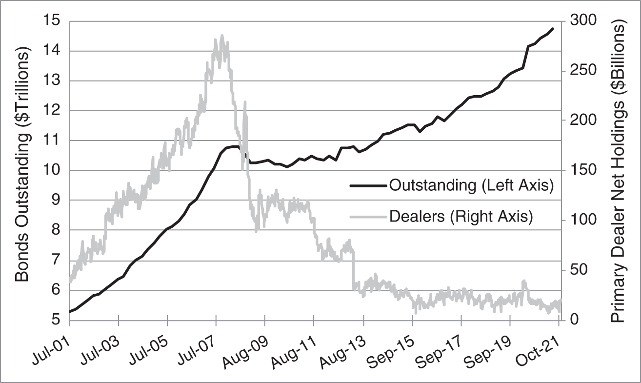
FIGURE 0.18 Primary Dealer Net Holdings of Corporate Bonds and Corporate Bonds Outstanding.
Sources: Primary Dealer Statistics, Federal Reserve Bank of New York; and Financial Accounts of the United States, Board of Governors of the Federal Reserve.
Growth of PTFs
In the Treasury market, the reduction of dealer market making has been made up, at least in part, by PTFs. These firms typically trade to make money on their accounts and try to make relatively small amounts of money on each of very many trades. They are often high‐frequency trading firms (HFTs) as well, but do not have to be. In any case, the PTF business model or trading style relies heavily on electronification, and the advance of electronification is in good part due to demand from PTFs. Market participants were shocked in 2015 by an inadvertent leak of the top 10 firms by trading volume on the largest platform for the electronic trading of Treasuries: only two were banks. Figure 0.19 uses more recent data to show how PTFs have grown in prominence in the Treasury market. Over the sample period, PTFs and dealers each comprised 48% of trading in the interdealer broker market (with buy‐side firms, like asset managers, comprising the remainder). Furthermore, true to their usual nature, about 93% of PTF trades were electronic, compared with 58% of dealer trades. Note, by contrast, that only 18% of buy‐side trades were electronic.
Growth of ETFs
Shares of an ETF represent fractional holdings of the fund's underlying portfolio and trade on an exchange. Authorized Participants (APs) of an ETF can create ETF shares by buying underlying assets, adding them to the fund's portfolio, and selling ETF shares against those additional assets. APs can also reduce the number of outstanding ETF shares by taking assets from the underlying portfolio, selling them, and purchasing existing ETF shares corresponding to the sold assets. An ETF has a NAV, usually expressed as a value per share, which is an estimate of the value of the underlying portfolio. However, investors buy or sell shares of an ETF on an exchange at a market‐determined price, which may be greater than, equal to, or less than the NAV. Unlike APs, investors cannot exchange their shares for securities in the underlying portfolio, nor can they deliver securities in exchange for new ETF shares.
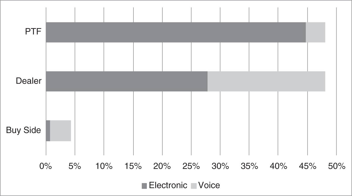
FIGURE 0.19 Percentages of Trading Volume in the Interdealer Broker Markets for Treasuries, by Participant Type and Trading Protocol, April to December 2019.
Source: Harkrader, J., and Puglia, M. (2020), “Principal Trading Firm Activity in Treasury Cash Markets,” FEDS Notes, Board of Governors of the Federal Reserve System, August 4.
ETFs in general, including fixed income ETFs, have experienced phenomenal growth. The first fixed income ETF was listed in 2002, and, by the end of 2020, assets under management in global bond ETFs exceeded $1.5 trillion.39 An important motivation for bond ETFs is the creation of liquid trading vehicles from relatively illiquid assets. As discussed earlier, in part because there are so many distinct corporate bond issues, individual corporate bonds are relatively illiquid, particularly as they age. By contrast, a small number of large and diversified portfolios, traded on exchanges and traded electronically in the form of ETFs, can be very liquid. Furthermore, growing liquidity and electronic trading in ETFs drive more electronic trading of corporate bonds, which further improves ETF liquidity, and so forth. In fact, a market has developed for trading portfolios comprising bonds that are all or mostly all held by ETFs.40 In any case, Figure 0.20 illustrates the liquidity advantages of ETFs. For each asset class shown, ETF assets under management (AUM) are a small fraction of total amounts outstanding. At the same time, however, ETF ADV is a large fraction of total ADV. For example, ETFs hold only 4.8% of high‐yield corporate bonds outstanding, but the ADVs of these ETFs comprise 24.3% of the ADV of all such bonds. In other words, high‐yield corporate bond ETFs are significantly more liquid than high‐yield corporate bonds.
Skeptics have argued that day‐to‐day ETF liquidity lulls investors into a false sense of security, in the sense that, under stressed market conditions, ETF liquidity will revert to the liquidity of the underlying bonds and essentially disappear. This theory was tested in March 2020, when markets roiled from the COVID pandemic and economic shutdowns. Underlying bond market liquidity did evaporate, with even primary issues of both investment‐grade and high‐yield bonds coming to a halt. Over the same time, however, ETF trading volumes increased dramatically. In other words, investors could not trade individual bonds, but could trade ETFs. The pricing of ETFs over the period, however, surprised some observers. As bond prices plummeted, ETFs traded at significant discounts from NAV; that is, the prices of the ETFs were very much below the estimated value of their underlying portfolios. Similarly, when bond prices rapidly recovered, ETFs traded at significant premiums to NAV, that is, at prices well above estimated portfolio values. Critics took this pricing behavior as evidence that ETFs were not working well, in the sense that investors could not trade shares at their true values. But by the definition of illiquidity during stress events, “true values” of individual bonds cannot be accurately determined at those times. It is most likely, therefore, that observed discounts from NAV resulted from stale bond prices: as prices swiftly fell with nearly no liquidity, bond prices recorded for the purposes of estimating NAV were stale, higher prices. Similarly, as prices rebounded quickly with little liquidity, NAV was estimated with stale, lower prices, making it seem that ETFs traded at a premium. Supporting this narrative was the fact that when prices were falling and ETFs were selling at a discount to NAV, investors were nevertheless giving bonds to APs to create new ETFs. Despite the apparent loss in value, investors could sell their bonds most efficiently by first exchanging them into ETFs.41
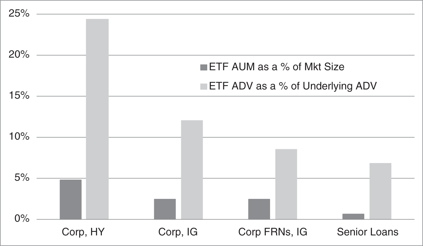
FIGURE 0.20 Exchange‐Traded Fund AUM and ADV as a Percentage of Market AUM and ADV.
Source: State Street Global Advisors (2020), “Fixed Income ETFs: Fact versus Fiction (Answers on Fund Structure, Liquidity, Trading and Performance),” June.
Growing Concentration of Asset Managers
Concentration in the asset management industry has been growing for some time. Assets under management at the top 20 global managers were 29% of total assets in 1995, 38% in 2000, and 43% in 2020. Furthermore, in 2020, the top 10 global managers managed 31% of total assets, and the top five, 21%. With respect to flows, a 2018 study found that 42% of asset management trading in investment‐grade corporate bonds came from the top five managers.42 Increasing concentration in asset management implies a growing demand in the market for larger trades or, equivalently, a growing amount of execution risk from having to break up large orders into smaller transactions.
Summary of Trends
The trends just presented can be combined into the following narrative. Dealers are allocating less risk to market making, while asset managers need to execute larger and larger trades. Therefore, dealers focus on their largest and best clients, pushing others to electronic platforms. The growth of PTFs makes up for some of the liquidity withdrawn by dealers, but by providing frequent liquidity on small trades rather than by assuming the execution risk of larger orders. The net results of these intersecting trends, therefore, are as follows:
- Liquidity has become plentiful for small trades in relatively liquid, electronic markets.
- Liquidity can still be challenging for larger trades, even in relatively liquid markets, and, of course, for trades in less liquid markets.
- More customers must bear the execution risk of their own trades, instead of paying dealers to assume this risk.
Liquidity and Fragility
The changing nature of liquidity in bond markets has raised the issue of market resilience or, its reverse, market fragility. In particular, some believe that liquidity provision by PTFs is less stable than by dealers. The argument is that PTFs will shut down in stress conditions, so as to avoid any losses on their own accounts, while dealers will continue to make markets for their clients, with whom they have ongoing and valuable business relationships. The “flash rally” in the Treasury market on October 15, 2014, provided a case study in which to examine this argument.
On that day, there was a release of retail sales data at 8:30am, but it is generally agreed that the news was not particularly surprising. Nevertheless, Treasury yields dropped relatively steeply over the next hour or so. Then, over the 12 minutes from 9:33am to 9:45am, the yield on the 10‐year Treasury fell by 16 basis points and then rose by 16 basis points (i.e., prices rose by a lot and then fell by a lot). This was an extremely large move for such a short time period – the daily standard deviation of the 10‐year yield was perhaps four or five basis points per day. Was any particular group of market participants to blame for this flash rally? Does the event forewarn of worse occurrences to come?
Subsequent analysis showed that over the 12 minutes in question, trading volume increased dramatically and market depth dropped precipitously. In other words, trading continued throughout the interval, and in large quantities, but through very many small orders and a consistent replenishment of limit orders. Market depth provided by both PTFs and dealers fell during the window. While market depth supplied by PTFs fell by a much larger percentage, PTFs supplied much more of the total throughout. Furthermore, PTFs did not change their bid–ask spreads by much, while dealers did at times. A joint study of regulators concluded that: “In very broad terms…PTFs, as a group, reacted…primarily by reducing limit order quantities, while the bank‐dealers reacted by widening bid–ask spreads and, for brief periods of time, removing their offers to sell securities.”43 Evidence from the flash rally, therefore, is consistent with the different nature of liquidity provision by PTFs and dealers; is not consistent with PTFs closing shop during a stress event; and is consistent with a liquidity regime that is shifting execution risk to the buy side.
There was a similar flash event on February 25, 2021, though this time Treasury prices fell significantly and then recovered in a short amount of time. The event was again characterized by sharply reduced market depth and sharply elevated trading volumes, that is, by rapid replenishment of limit orders.44 The extent to which markets are susceptible to similar and perhaps worse occurrences remains a topic of concern.
NOTES
- 1 The data sources are different, but the inclusion of nontraded instruments here is the main discrepancy between this $76.4 trillion total and the $48 trillion total of US debt securities in Figures 0.1 and 0.2. In particular, adding to that $48 trillion the $6.8 trillion of nonmarketable Treasury securities, $7.8 trillion of nonsecuritized mortgages, $9.0 trillion of loans and advances, and $4.3 trillion of consumer credit gives a total of about $76 trillion.
- 2 Over a period of deflation, TIPS principal amount may fall below original principal for the purposes of calculating interest, but, at maturity, TIPS return at least the original principal amount.
- 3 While there would seem to be no particular need to lock in longer‐term funding, because the US Treasury has never had a problem rolling over its short‐term borrowings, prudent debt management avoids scenarios in which too much debt matures and needs to be refinanced over a relatively short period of time.
- 4 A basis point is 0.01%. The difference between a rate of 1.01% and 1.00% is one basis point, and a rate of 1% might be referred to as a rate of 100 basis points. The spread of five basis points in the text, therefore, is a spread of 0.05%.
- 5 Historically, municipalities had been allowed to refinance existing tax‐exempt debt in advance of maturity or any call option with the proceeds of new, tax‐exempt debt, but this practice was outlawed in 2017. For a full treatment of this and other related issues, see Kalotay, A. (2021), Interest Rate Risk Management of Municipal Bonds, Andrew Kalotay Associates, Inc.
- 6 When a municipality defeases a tax‐exempt bond issue, it needs to purchase Treasury securities, but is prohibited – to prevent tax arbitrage at the expense of the federal government – from investing at a higher rate than the rate on the defeased, tax‐exempt issue. This problem is solved by purchasing SLUGs directly from the Treasury, which are mentioned earlier in the chapter. SLUGs are the same credit quality as other Treasuries but pay a lower interest rate to suit the needs of the particular defeasance.
- 7 See Gillers (2020), “Bond Insurance Returns to the Muni Market in a Big Way,” The Wall Street Journal, October 22; and Moran, D. (2020), “Municipal Bond Insurance Busier Than Ever After Decade‐Long Slump,” Insurance Journal, June 26.
- 8 Because many of the MBS issued by the Federal National Mortgage Association (FNMA) and the Federal Home Loan Mortgage Corporation (FHLMC) have been consolidated on to their balance sheets, the Financial Accounts of the United States include these as part of the debt of government‐sponsored enterprises (GSEs). Figure 0.4 and the numbers in this paragraph exclude these MBS from Agency/GSE debt so as not to double count the underlying mortgages.
- 9 The household sector, in this data set, includes private equity funds, domestic hedge funds, personal trusts, and nonprofits, with combined assets that could easily exceed $10 trillion. Their inclusion here results in some overstatement of the extent to which individuals invest directly in equity and debt markets.
- 10 Home equity loans are second liens, which are subordinate to first home mortgages with respect to creditor priority.
- 11 See, for example, Amir, E., Teslow, J., and Borders, C. (2021), “The MeasureOne Private Student Loan Report,” June 15.
- 12 With respect to competitiveness, note that concentration within the banking sector does not, on its own, account for competition with nonbanking entities, like money market funds, nonbank mortgage lenders, and some fintech firms.
- 13 Employee Benefits Security Administration (2021), “Private Pension Plan Bulletin Historical Tables and Graphs, 1975–2019,” September.
- 14 Wadia, Z., Perry, A., and Clark, C. (2021), “2021 Corporate Pension Study,” Milliman White Paper, April.
- 15 Reserve Primary Fund shareholders eventually received 99.1 cents per share.
- 16 As an aside, the Dodd‐Frank Act of 2010 forbade the Treasury's use of its Exchange Stabilization Fund to guarantee money market funds. In March 2020, Congress lifted this ban through the end of 2020. Dodd‐Frank also required that the Federal Reserve's emergency facilities for nonbanks have “broad‐based eligibility” and be approved by the Secretary of the Treasury.
- 17 See Sidley (2022), “SEC Proposes New Rule Amendments for Money Market Funds,” January 3.
- 18 The Federal Reserve System includes 12 Federal Reserve banks, spread around the country, and the Board of Governors, in Washington, D.C.
- 19 As mentioned earlier, a repo is a loan collateralized by a security. In the context of the text, repos with the Fed are all collateralized by government‐guaranteed securities.
- 20 Interview of Ben Bernanke by Liaquat Ahamed, “Central Banking after the Great Recession,” Brookings, January 16, 2014.
- 21 Chapter 12 describes the current, limited trading in the fed funds market.
- 22 The Fed recently substituted Interest on Excess Reserves (IOER) with IORB. Also, the system of setting rates described in the text is sometimes called a “floor” system, because reserves are so plentiful that, between the relatively high discount window rate at which banks can borrow from the Fed, and the relatively low IORB at which banks can lend to the Fed, the market interest rate equals the lower IORB. In a “corridor” system, by contrast, reserves would be calibrated such that the market interest rate settles between the discount window rate and the IORB.
- 23 In a reverse repo, a counterparty lends money and “reverses in” securities (see Chapter 10). Hence, the counterparties that are lending money to the Fed are doing reverse repo.
- 24 For a fuller discussion of monetary policy with abundant reserves and repo markets in September 2019, see Copeland A., Duffie, D., and Yang, Y. (2021), “Reserves Were Not So Ample After All,” Staff Report Number 974, Federal Reserve Bank of New York, July; and Nelson, B. (2022), “The Fed Is Stuck on the Floor: Here's How It Can Get Up,” Bank Policy Institute, January 11.
- 25 With respect to this episode, see, for example, Baer, J. (2020), “The Day Coronavirus Nearly Broke the Financial Markets,” The Wall Street Journal, May 20; and Duffie, D. (2020), “Still the World's Safe Haven?” Hutchins Center Working Paper #62, May.
- 26 And one of the reasons the Treasury has been holding greater cash balances is its wanting a cushion against the occasional political stalemates with respect to raising the debt ceiling, which, by limiting new borrowing, can leave the Treasury scrambling for cash.
- 27 In theory, an investor could buy a negative yielding bond by paying its face amount, paying a periodic coupon, and then receiving the face amount at maturity. It is not feasible, however, for a government or corporate issuer to track down individual investors to collect coupon payments. Therefore, bonds with negative yields are sold as described in the text, with an initial price above par, a coupon of zero, and a return of par.
- 28 See, for example, Flood, C. (2021), “In Charts: Bonds with Negative Yields Around the World,” Financial Times, September 27.
- 29 The ECB also sets a rate for borrowing through its marginal lending facility, which is the equivalent of the discount window at the Fed.
- 30 See, for example, Beauregard, R., and Spiegel, M. (2020), “Commercial Banks Under Persistent Negative Rates,” FRBSF Economic Letter 2020–29, Federal Reserve Bank of San Francisco, September 28; and Kowsmann, P. (2021), “Banks in Germany Tell Customers to Take Deposits Elsewhere,” The Wall Street Journal, March 1.
- 31 These include €318 billion held under the Commercial Sector Purchase Programme (CSPP), as of early February 2022, and €50 billion under the Pandemic Emergency Purchase Programme (PEPP), as of the end of November 2021.
- 32 “For purchases under the PEPP…the benchmark allocation…will be guided by the [capital] key[s]…A flexible approach to the composition of purchases…is nonetheless essential…” Source: Decision (EU) 2020/440 of the European Central Bank of 24 March 2020 on a temporary pandemic emergency purchase programme (ECB/2020/17), paragraph (5).
- 33 Ainger, J. (2020), “One of the World's Top Bond Markets Slowly Capitulating to QE,” December 9; Reuters (2021), “UPDATE‐1‐ECP Buys More Bonds Than Countries Sell to Cap Yields,” August 2.
- 34 The SURE bonds are “social bonds,” or an environmental, social, and governance (ESG) debt instrument, and €250 billion of the NextGenerationEU bonds will be green bonds, used to fund eligible projects. This issue of green bonds will make the EC the world's largest issuer of green bonds.
- 35 Statistics cited in this paragraph are from: Blackrock (2017), “The Next Generation Bond Market;” Theisen, S. (2018), “Developments in Credit Market Liquidity,” SEC FIMSAC Meeting, Citi, January 11; and MSRB (2019), “Municipal Securities Rulemaking Board 2019 Fact Book.”
- 36 Customers and dealers participating in RFQs have typically known each other's identities. Recently, however, anonymous RFQ platforms have gained traction.
- 37 Mackenzie, M. (2021), “Pandemic's Digital Push Shows Future of Bond Trading,” Financial Times, November 7; McPartland, K. (2021), “All‐to‐All Trading Takes Hold in Corporate Bonds,” Greenwich Associates, Second Quarter; McPartland, K., Monahan, K., and Swanson, S. (2020), “US Capital Markets Performance During COVID,” Greenwich Associates, December 22; Wiltermuth, J. (2021), “Electronic Trading in US Corporate Bonds Is Finally Taking Off,” MarketWatch, July 14; and Author Calculations.
- 38 Primary dealers commit to participate in Treasury auctions and are trading counterparties and market makers for the Fed.
- 39 iShares by Blackrock (2021), “By the Numbers: New Data Behind the Bond ETF Primary Process.”
- 40 Mackenzie, M. (2021), “Pandemic's Digital Push Shows Future of Bond Trading,” Financial Times, November 7.
- 41 For accounts of ETFs during March 2020, see, for example: Aramonte, S. and Avalos, F. (2020), “The recent distress in corporate bond markets: cues from ETFs,” BIS Bulletin No. 6, April 14; Levine, M. (2020), “Money Stuff: The Bull Market Caught a Virus,” Liquidity Illusion Illusion, Bloomberg, March 12; and S&P Global Ratings (2020), “Credit Trends: How ETFs Contributed to Liquidity and Price Discovery in the Recent Market Dislocation,” July 8.
- 42 McPartland, K. (2019), “The Challenge of Trading Corporate Bonds Electronically,” Greenwich Associates, Q2; Thinking Ahead Institute (2020), “Global Asset Manager AuM tops US$100 Trillion for the First Time,” Willis Towers Watson, October 19; and Author Calculations.
- 43 Joint Staff Report (2015), “The US Treasury Market on October 15, 2014,” p. 28.
- 44 Aronovich, A., Dobrev, D., and Meldrum, A. (2021), “The Treasury Market Flash Event of February 25, 2021,” FEDS Notes, Board of Governors of the Federal Reserve System, May 14.