Natural Detail
Many phenomena found in nature don’t conform well to simple geometric representations. Many of these objects, such a fire and smoke, have complex internal motions and indistinct borders. Others, such as a cloud layer and a lake surface, can have boundaries, but these boundaries are constantly changing and are complex in shape. This chapter focuses on these amorphous objects, extending OpenGL’s expressive power by harnessing techniques such as particle systems, procedural textures, and dynamic surface meshes.
Given the complexity in detail and behavior of the objects being modeled, tradeoffs between real-time performance and realism are often necessary. Because of this, performance issues will often be considered, and many of the techniques trade-off some realism in order to maintain interactivity. In many ways, these techniques are simply building blocks for creating realistic natural scenes. Producing extreme realism requires careful attention to every aspect of the scene. The costs, both in development time and application performance, must be managed. High realism is best applied where the viewer will focus the most attention. In many cases, it is most effective to settle for adequate but not spectacular detail and realism in regions of the scene that aren’t of central importance.
18.1 Particle Systems
A “particle system” is the label for a broad class of techniques where a set of graphics components is controlled as a group to create an object or environment effect. The components, called particles, are usually simple,—sometimes as simple as single pixels. Particle systems are used to represent a variety of objects, from rain, smoke, and fire to some very “unparticle-like” objects such as trees and plants.
Given the broad range of particle system applications, it’s risky to make definitive statements about how they should be implemented. Nevertheless, it’s still useful to describe some particle system techniques and guidelines, with the caveat that any rules on the proper use of particles will undoubtedly have exceptions.
A number of objects can be represented well with particles systems. Objects such as rain, snow, and smoke that are real-life systems of particles are a natural fit. Objects with dynamic boundaries and that lack rigid structure—such as fire, clouds, and water—also make good candidates.
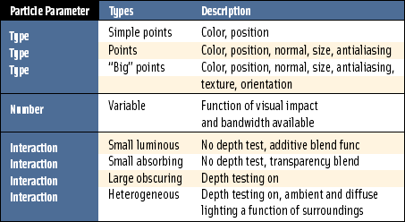
The appearance of a particle system is controlled by a number of factors: the number and appearance of the particles themselves, the particles’ individual behaviors, and how the component particles “interact.” Each factor can vary widely, which allows particle systems to represent a wide range of objects. Table 18.1 provides some examples on how particles systems can vary in their characteristics.
The ways parameters can be made to change over time is almost unlimited, and is a key component to particle systems’ expressive power. A fundamental technique for modifying particles’ behavior over time is parameterization. A particle’s position, color, and other characteristics are controlled by applying a small number of temporal or spatial parameters to simple functions. This makes it easier to orchestrate the combined behavior of particles and boosts performance. If the global behavior of the particle system is sufficiently constrained, difficult-to-calculate characteristics such as local particle density, can become a simple function of a position or distance parameter.
Particle interaction is controlled by how their attributes are orchestrated, and by rendering parameters. Luminous small particles (such as fire) can be approximated as transparent and luminous, and so can be rendered with depth testing off using an additive blend. Obscuring fine particles, such as dust, can also be rendered without depth (which helps performance), using a normal replace operation. More sophisticated lighting models are also possible. A particle deep inside a dense cloud of particles can be assumed to be lighted only with ambient light based on the color of the surrounding particles. Particles on the outside of a cloud, in a region of lower density, can be lighted by the environment, using diffuse or even specular components.
Despite their power, particle systems have significant limitations. Primary is the performance penalty from modifying and rendering a very large number of graphics primitives each frame. Many of the techniques used in particle systems focus on maximizing the efficiency of updating particle attributes and rendering them efficiently. Since both the updating and rendering steps must be performed efficiently to use a particle system effectively, both processes are described here.
18.1.1 Representing Particles
Individual particles can range from “small” ones represented with individual pixels rendered as points, to “big” once represented with textured billboard geometry, or even complete geometric objects, such as tetrahedrons. The parameters of an individual particle can be limited to position and color, or can incorporate lighting, texture, size, orientation, and transparency. The number of objects varies depending on the effect required and performance available. In general, the more internal variation and motion that has to be expressed the more particles are required. In some cases, a smaller number of big particles can be used, each big particle representing a group of smaller ones.
Big Particles
The choice of particle is often a function of the complexity of the object being represented. If the internal dynamics of an object vary slowly, and the object has a relatively well-defined boundary, a smaller number of “big” particles may represent the object more efficiently. A big particle represents a group of the objects being modeled. The particle is sized so that its rigidity doesn’t detract from adequately modeling the dynamics of the object.
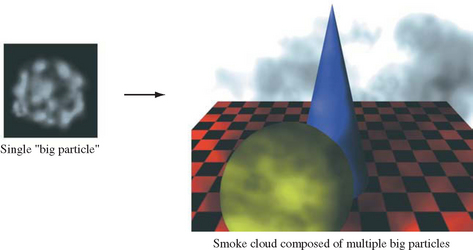
Sometimes big particles are a more realistic choice than small ones. Smoke, for example, consists of individual particles that are invisible to the viewer, even when close up. A big particle can contain an image that accurately represents the appearance of a puff of smoke, which would be expensive and difficult to do by controlling the properties of individual pixels. The key requirement is combining big particles and controlling their properties so that they combine seamlessly into the desired object.
Big particles are usually represented as textured and billboarded polygons, in order to minimize vertex count. Because they are composed of multiple vertices, the application can have a great deal of control over the particle’s appearance. Textures can be applied to the particles, and color and lighting can vary across their surfaces. The particle outlines can be stenciled into arbitrary shapes with alpha component textures, and the particles can be oriented appropriately.
Good examples of objects that can be modeled with big particles are vapor trails, clouds, and smoke. In these cases, the object can be decomposed into a small number of similar pieces, moving in an orchestrated pattern. The objects in these examples are assumed to have a low amount of turbulence, relatively high opacity, and fairly well-defined boundaries. Big particles become overlapping “patches” of the object, moving independently, as shown in Figure 18.1.
The geometry of big particles are simple polygons, usually quads, that are transformed using the billboard technique described in Section 13.5. The polygons are covered with a surface texture containing an alpha component. This makes it possible to vary the transparency of the polygon across its surface, and to create an arbitrary outline to the polygon without adding vertices, as described in Section 6.2.2.
Big particles can be controlled by varying a few important characteristics. Unifying and simplifying the potential parameters makes it possible to manage and update a large number of particles every frame. Fortunately, the particle system paradigm holds true: a few particle parameters, applied to a large number of particles, can yield significant expressive power. Table 18.2 shows a useful set of big-particle parameters. Note that the parameters are chosen so that they are inexpensive to apply. None of them, for example, requires changing the geometric description of the particle. Size and orientation can be changed by modifying the particle’s modeling transform. Binding textures to particles can be expensive, but the number of textures used is small (often one). A single texture map is often applied to large groups of particles, amortizing the cost. The textures themselves are also small, making it possible to keep them resident in texture memory.
Table 18.2
| Parameter | Description |
| Size | Scale factor of polygon |
| Orientation | Rotation around axis pointing to viewer |
| Current texture | Small number of textures shared by many particles |
| Color | All vertices same color; can modify texture (using modulate) |
| Lighting | Light enables and light position; shared by many particles material and normals usually held constant |
Current color can be changed for groups of particles, if there is no color associated with the particle geometry. Color is changed by updating the current color before rendering a group of particles. If the texture environment is set to combine texture and polygon color, such as GL_BLEND or GL_MODULATE, the current color can be used to globally modify the particle’s appearance. Lighting can be handled by changing the current state, as is done for color. Color material can also be used to vary material properties. Lights can be enabled or disabled, and lighting parameters changed, before rendering each group of particles. Geometric lighting attributes, such as vertex normals and colors, are supplied as current state, or are part of the per-vertex geometry and kept constant.
Small Particles
While big particles can model an important class of objects efficiently, approximating an object with a small number of large, complex primitives isn’t always acceptable. Some objects, particularly those with diffuse, highly chaotic boundaries, and complex internal motion, are better represented with a larger number of smaller particles. Such a system can model the internal dynamics of the object more finely, and makes the representation of very diffuse and turbulent object boundaries and internal structure possible. Small particles are a particularly attractive choice if the individual particles are large enough to be visible to the viewer, at least when they are nearby. Examples include swarms of bees, sparks, rain, and snow.
A good candidate primitive for simple particles is the OpenGL point. Single points can be thought of as very inexpensive billboards, since they are always oriented toward the viewer. Although simple particles are often small, it’s still useful to be able to provide visual cues about their distance by varying their size. This can be done with the OpenGL point size parameter. Changing size can become a challenge when trying to represent a particle smaller than a single pixel. Subpixel-size particles can be approximated using coverage or transparency. With OpenGL, this is done by modifying the alpha component of a point’s color and using the appropriate blending function.
Objects that are small compared to the size of a pixel can scintillate when moving slowly across the screen. Antialiasing, which controls pixel brightness as a function of coverage, mitigates this effect. OpenGL points can be antialiased; they are modeled as circles whose radius is controlled by point size. Changing point size, especially for antialiased points, can be an expensive operation for some implementations, however. In those cases, techniques can be used to amortize the cost over several particles, as discussed in Section 18.3.
If the ARB_point_parameters extension is available1, an application can set parameters that control point size and transparency as a function of distance from the viewer. A threshold size can be set, that automatically attenuates the alpha value of a point when it shrinks below the threshold size. This extension makes it easy to adjust size and transparency of small particles based on viewer distance.
Point parameters shouldn’t be considered a panacea for controlling point size, however. Depending on how the extension is implemented, the same performance overhead for point size change could be hidden within the implementation. The extension should be carefully benchmarked to determine if the implementation can process a set of points with unsorted distance values efficiently. If not, the methods for amortizing point size changes discussed in Section 18.3 can also be used here.
A more recent extension, GL_ARB_point_sprite, makes OpenGL points even more versatile for particle systems. It adds special point sprite texture coordinates that vary from zero to one across the point. Point sprites allow points to be used as billboard textures, blurring the distinction between big and small particles. A point sprite allows a particle to be specified with a single vertex, minimizing data transfer overhead while allowing the fragments in the point to index the entire set of texels in the texture map.
Antialiasing Small Particles
Particles, when represented as points, can be spatially antialiased by simply enabling GL_POINT_SMOOTH and setting the appropriate blending function. It can also be useful to temporally antialias small particles. A common method is to “stretch” them. The particle positions between two adjacent frames are used to orient an OpenGL line primitive centered at the particle’s current position. A motion blur effect (Section 10.7.1) is created by varying the line’s length and alpha as a function of current velocity. Lines are a useful particle primitive in their own right. Like points, they can be thought of a billboarded geometry. Their size can be controlled by adjusting their width and length, and they can be antialiased using GL_LINE_SMOOTH.
If high quality is critical and performance isn’t as important, or the implementation has accelerated accumulation buffer support, the accumulation buffer can be used to generate excellent particle antialiasing and motion blur. The particles for a given frame can be rendered repeatedly and accumulated. The particle positions can be jittered for spatial antialiasing, and the particle rerendered along its direction of motion to produce motion blur effects. For more information, see Section 10.2.2, and the accumulation buffer paper (Haeberli, 1990).
18.1.2 Number of Particles
After the proper particle type and characteristics are chosen, the next step in designing a particle system is to choose the number of particles to display. Two issues dominate this design decision: the performance limitations of the system, and the degree of complexity that needs to be modeled in the object. There are cases where fewer particles are called for, even if the implementation can support them. For example, if a particle system is being used to represent blowing dust, the number of particles should match the desired dust density. Too many particles can average together into a uniform block of color, destroying the desired effect.
Performance limitations are the simplest limitation to quantify. Benchmarking the application is key to determining the number of particles that can be budgeted without overwhelming the graphics system rendering them, and the CPU updating them. Often performance constraints will dictate the number of particles that can be rendered.
18.1.3 Modeling Particle Interactions
Independently positioning and adjusting the other parameters of each particle in isolation typically isn’t sufficient for realistic results. Controlling how particles visually interact is also important. Unless the particles are very sparse, they will tend to overlap each other. The color of particles may also be affected by the number of other particles there are in the immediate vicinity.
Choosing how particles interact is affected by the physical characteristics of the particles being modeled. Particles can be transparent or opaque, light absorbing or light emitting, heterogeneous or homogeneous. Fine particles are often assumed to be transparent, causing particles along the same line of sight to interact visually. Larger particles may block more distant ones. Transparent particles may emit light. In this case, any particles along the same line of sight will add their brightness. More absorbing particles along the same line of sight will obscure more of the scene behind the particles.
Some of these effects are shown in Figure 18.2. Three cubes of particles are drawn, each with the same colors, alpha values, and positions. The left cube draws them with no blending, representing lighted opaque particles that obscure each other. The center uses blending with the function GL_SRC_ALPHA, GL_ONE_MINUS_SRC_ALPHA, representing transparent particles. The right cube blends with GL_ONE, GL_ONE, representing glowing particles. Each cube is divided into four quadrants. The left side has a white background; the right side has a black one. The top half of each cube has a background with maximum depth values. The bottom half has background geometry closer to the eye, only one-quarter of the way from the front of the particle cube.
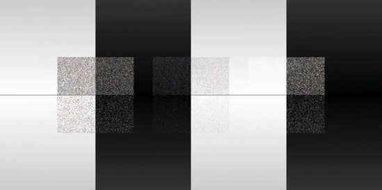
Although the particles are identical, they appear different depending on how they interact. The backgrounds are more visible with the transparent particles, with the center cube showing more background than the left one. The right cube, containing glowing particles, sums toward a constant value with areas of high particle density. The glowing particles stand out against the dark background and appear washed out when drawn in front of a white one.
Much of the visual interaction between particles can be controlled by using alpha components in their color and applying blend functions, or using depth buffering. Transparent luminous particles are rendered with an additive blend function and no depth updates. Absorbing particles are rendered with an appropriate alpha value, no depth updates, and with a blend function of GL_SRC_ALPHA and GL_ONE_MINUS_SRC_ALPHA. Larger, obscuring particles can be rendered with normal depth testing on and blending disabled. In cases where depth updates are disabled, the normal caveats discussed in Section 11.9 apply: the background geometry should be rendered first, with depth updates enabled.
Particles in a system may vary in appearance. For example, a dense cloud of particles may have different lighting characteristics depending on where they are in the cloud. Particles deep within the cloud will not have direct views of lights in the scene. They should be rendered almost entirely with an ambient light source modeling particle interreflections. Particles near the boundaries of the cloud will have a much lower, but still significant, ambient light contribution from other particles but will also be affected by lights in the scene that are visible to it.
Rendering particles with heterogeneous appearance requires accurately determining the proper lighting of each particle, and proper rendering techniques to display their colors. The first problem can be easy to solve if the particle system dynamics are well understood. For example, if a cloud’s boundaries are known at any given time the particle color can become a simple function of position and time. For a static, spherical object, the color could be a function of distance from the sphere’s center. Rendering heterogeneous particles properly is straightforward if depth buffering is enabled, since only the closest visible particles are rendered. If particles are transparent, the particle set must be sorted from back to front when a blend function, such as GL_SRC_ALPHA and GL_ONE_MINUS_SRC_ALPHA, is used, unless the particle colors are very similar.
18.1.4 Updating and Rendering Particles
Choosing the correct type and number of particles, their attributes, and their interactions is important for creating a realistic object, but that is only one part of the design phase. A particle system will only function correctly if the updates and rendering stages can be implemented efficiently enough to support the particle system at interactive rates.
An important bottleneck for particle systems is the bandwidth required to transfer the particle geometry to the graphics hardware. If simple particles suffice, OpenGL points have low overhead, since they require only a single vertex per point. The number of components and the data types of the components should also be minimized. Position resolution, rather than range, should be considered when choosing a coordinate type, since the transformation pipeline can be used to scale point position coordinates as necessary.
Reducing transfer bandwidth also demands an efficient method of representing the particle set. The fine-grain glBegin/glEnd command style requires too much function call overhead. Display lists are more efficient, but are usually a poor fit for the points that require individual attribute updates each frame. Vertex arrays are the preferred choice. They avoid the overhead of multiple function calls per-vertex, and have an additional advantage. The primitive data is already organized in array form. This is a common representation for particle attributes in a particle system update engine, allowing the particles to be operated on efficiently. Structuring the particle system so that attribute data can be passed directly to OpenGL avoids data conversion overhead.
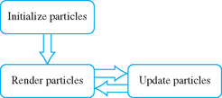
Particle system software has three basic components: initialization, rendering, and update (as shown in Figure 18.3). Particles in particle systems can be organized in tables, indexed by the particle, containing particle characteristics to be updated each frame (as shown in Table 18.3).
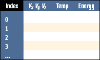
Using compact representations for both rendering and nonrendering parameters is important for performance reasons. A smaller array of parameters can be more easily held in the CPU cache during update, and can be transfered more efficiently to the graphics hardware. Using integer representations is helpful, as is factoring out parameters that are constant within a group of particles.
Parameters directly used for rendering, such as position and color, are best kept in tables separate from the nonrendering parameters, such as current velocity and energy. Many OpenGL implementations have faster transfer rates if the vertex arrays have small strides. Performance analysis and benchmarking are essential to determining which particle updating method is faster: using an incremental update algorithm and caching intermediate results (such as velocity) or performing a more computationally intensive direct computation that requires less stored data.
When choosing a vertex array representation, keep in mind that OpenGL implementations may achieve higher performance using interleaved arrays that are densely packed. The particle engine data structures may have to be adjusted to optimize for either rendering speed or particle update performance, depending on which part of the system is the performance bottleneck.
Sorting Particles
A bottleneck that can affect both transfer rate and rendering performance is OpenGL state changes. Changing transformation matrices, binding a new set of textures, or enabling, disabling, or changing other state parameters can use up transfer bandwidth, as well as add overhead to OpenGL rendering. In general, as many primitives should be rendered with the same state as possible.
One method to minimizing state changes is state sorting. Primitives that require the same OpenGL state are grouped and rendered consecutively. State sorting makes it possible to set an attribute, such as color, for a whole group of particles, instead of just one. Performance tuning methods are discussed in greater detail in Chapter 21.
As mentioned previously, an example of a state change that might require sorting is point size, since it can be a costly operation in OpenGL. The overhead can be minimized by sorting and grouping the particles by size before rendering to minimize the number of glPointSize calls. Sorting itself can lead to significant CPU overhead, and must be managed. It can be minimized in many cases by organizing the initial particle list, since their relative distances from the viewer may be known in advance.
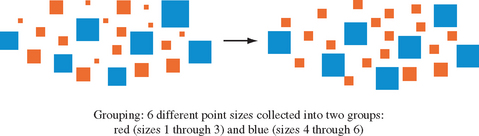
Sorting overhead can also be reduced by quantizing the parameter to be sorted. Rather than support the entire range of possible parameter values, find objects with similar parameter values and group them, representing them all with a single value. In Figure 18.4, a range of six different point sizes are combined into two groups, illustrated as “red” points (sizes 1 through 3) and “blue” points (sizes 4 through 6). In this example, the different red point sizes are collapsed into a single point size of 2, while the blue points are represented as points of size 5.
Quantizing simplifies sorting by reducing the number of possible different values. Point size changes may also be quantized to some degree. If particles are very small and of uniform size, bounding volumes can be chosen so that the particles within it are close together relative to their distance from the viewer. For a given bounding volume, an average point size can be computed, and all particles within the volume can be set to that size. The effectiveness of quantizing particle size this way will depend on the behavior of particles in a particular system. Particles moving rapidly toward or away from the viewer cannot be grouped effectively, since they will show size aliasing artifacts.
The sorting method used should match well with the particle system’s storage representation. Since the elements are in arrays, an in-line sorting method can be used to save space. An incremental sorting algorithm can be effective, since points usually move only a small distance from frame to frame. An algorithm that is efficient for sorting nearly sorted arrays is ideal, for example, insertion and shell sorts take linear time for nearly sorted input.
Because of their compact representation, many particle systems require a sort against key values that have a narrow range. In these cases, a radix-exchange sort may prove effective. Radix sort is attractive, since it uses n log n bit comparisons to sort n keys. The smaller the keys the better. The sort is guaranteed to use less than nb bit comparisons for n keys each with b bits.
In some cases, such as presorting to work around an inefficient implementation of glPointParameter, it may be possible to only partially sort particles and still get useful results. Partial sorting may be necessary if an interactive application can only spare a limited amount of time per frame. In this case, sorting can proceed until the time limit expires. However, it must be possible to interrupt the sorting algorithm gracefully for this approach to work. It is also important for the sort to monotonically improve the ordering of the particles as it proceeds. In the glPointParameter example, some sorting can improve rendering performance, even if the sort doesn’t have time to complete.
Vertex Programs
If the OpenGL implementation supports vertex programs, some or all particle updating can be done by the OpenGL implementation. A vertex program can be created that uses a global parameter value representing the current age of all particles. If each particle is rendered with a unique vertex attribute value, a vertex program can use the current parameter value and vertex attribute as inputs to a function that modifies the position, color, size, normal, and other characteristics of the particle. Since each particle starts with a different attribute, they will still have different characteristics. Each time the frame is rendered, the global parameter value is incremented, providing an age parameter for the vertex program.
Using vertex programs is desirable since updates are happening in the implementation. Depending on the implementation this work may be parallelized and accelerated in hardware. It also keeps the amount of data transferred with each particle to a minimum. The trade-off is less flexibility. Currently, vertex programs don’t support decision or looping constructs, and the operations supported, while powerful, aren’t as general as those available to the application on the CPU.
18.1.5 Applications
The following sections review some common particle system applications. These descriptions help illustrate the application of particle system principles in general, but also show some of the special problems particular to each application.
Precipitation
Precipitation effects such as rain and snow can be modeled and rendered using the basic particle rendering techniques described in the preceding section. Using snowflakes as an example, individual flakes can be rendered as white points, textured billboards, or as point sprites. Ideally, the particle size should be rendered correctly under perspective projection. Since the real-life particles are subject to the effects of gravity, wind, thermal convection, and so on, the modeled dynamics should include these effects. Much of the complexity, however, lies in the management of the particle lifetime. In the snow example, particle dynamics may cause particles to move from a region not visible to the viewer to a visible portion, or vice versa. To avoid artifacts at the edges of the screen, more than the visible frustum has to be simulated.
One of the more difficult problems with particle systems is managing the end of life of particles efficiently. Usually snowflakes accumulate to form a layer of snow over the objects upon which they fall. The straightforward approach is to terminate the particle dynamics when the particle strikes a surface (using a collision detection algorithm), but continue to draw it in its final position. But this solution has a problem: the number of particles that need to be drawn each frame will grow over time without bound.
Another way to solve this problem is to draw the surfaces upon which the particles are falling as textured surfaces. When a particle strikes the surface, it is removed from the system, but its final position is added to a dynamic texture map. The updated texture is reapplied to the snow-covered surface. This solution allows the number of particles in the system to reach a steady state, but creates a new problem: efficiently managing the texture maps for the collision surfaces.
One way to maintain these texture maps is to use the rendering pipeline to update them. At the beginning of a simulation the texture map for a surface is free of particles. At the end of each frame, the particles to be retired this frame are drawn with an orthographic projection onto the textured surface (choosing a viewpoint perpendicular to it) using the current version of the texture. The resulting image replaces the current texture map.
There is a problem transitioning from a particle resting on the surface (which is really a billboarded object facing the viewer) and the texture marked with the new snow spot. In general, the textured surface will be at an oblique angle with the viewer. Projecting the screen area onto the texture will lead to a smooth transition, but in general the updated texture area won’t look correct from any other viewing angle. A more robust solution is to transition from particle to texture spot using a multiframe fade operation. This will require introducing a new limbo state for managing particles during this transition period.
Using a texture map for snow particles on the surface provides an efficient mechanism for maintaining a constant number of particles in the system and works well for simulating the initial accumulation of precipitation on an uncovered surface. However, it does not serve as a realistic model for continued accumulation since it only simulates a 1D layer. To simulate continued accumulation, the model would have to be enhanced to simulate the increasing accumulation thickness. Modifying the surface with a dynamic mesh (as described in Section 18.2) is one possible solution.
When simulating rain instead of snow, some of the precipitation properties change. Rain particles are typically denser than snow particles and are thus affected differently by gravity and wind. Since heavy rain falls faster than snow, it may be better simulated using short antialiased line segments rather than points, to simulate motion blurring.
Simulating the initial accumulation of rain is similar to simulating snow. In the case of snow, an opaque accumulation is built up over time. For rain, the raindrops are semi-transparent; they affect the surface characteristics and thus the surface shading of the collision surface in a more subtle manner. One way to model this effect is to create a gloss map, as described in Section 15.7.1. The gloss map can be updated per particle, as was done in the snow example, increasing the area of specular reflection on the surface.
For any precipitation, another method to reduce the rendering workload and increase the performance of the simulation is to reduce the number of particles using a “Hollywood” technique. In this scheme, rather than rendering particles throughout the entire volume a “curtain” of particles is rendered in front of the viewer. The use of motion blurring and fog along with lighting to simulate an overcast sky can make the illusion more convincing. It is still possible to simulate simple accumulation of precipitation by choosing points on collision surfaces at random (within the parameterization of the simulation), rather than tracking particle collisions with the surfaces, and blending them into texture maps as described previously.
Smoke
Exactly modeling smoke requires some sophisticated physics, but surprisingly realistic images can be generated using fairly simple techniques. One such technique uses big particles; each particle is textured with a 2D cross section of a puff of smoke. To simplify manipulation, a texture containing only luminance and alpha channels can be used. If the GL_MODULATE texture environment is used, changing the color and alpha value of the particle geometry controls the color and transparency of the smoke. Controlling the appearance of the smoke with geometry attributes, such as vertex color, also makes it possible to simulate different types of smoke with the same texture. While smoke from an oil fire is dark and opaque, steam from a factory smoke stack is much lighter in color.
The size, position, orientation, and opacity of the particles can be varied as a function of time to simulate the puff of smoke enlarging, drifting, and dissipating over time (see Figure 18.5). Overlapping the smoke particles creates a smokey region of arbitrary shape, which can be modified dynamically over time by moving, rotating, scaling, and modifying the color and transparency of the component particles.
The smoke texture, used to represent a group of smoke particles, is a key building block for building smoke effects of this type. The texture image itself may vary. A single texture may be used for all particles. The texture used can vary with particle position, or might be animated over time, depending on the requirements of the application. The realism and accuracy of the texture image itself is important. There are a number of procedural techniques that can be used to synthesize both static and dynamic 2D textures, as described in Section 18.3. Some of the literature devoted to realistic clouds, as described in Section 18.6, can also be applied to producing smoke textures.
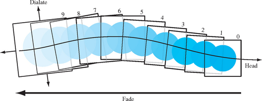
Vapor Trails
Vapor trails emanating from a jet or a missile can be modeled with a particle system, treating it as a special case of smoke. A circular, wispy 2D smoke texture applied on a big particle is used to generate the vapor pattern. The texture image can consist of only alpha components, modulating the transparency of the image, letting the particle geometry set the color. The trajectory of the vapor trail is painted using multiple overlapping particles, as shown in Figure 18.6. Over time the individual billboards gradually enlarge and fade. The program for rendering a trail is largely an exercise in maintaining an active list of the position, orientation, and time since creation for each particle used to paint the trail. As each particle exceeds a threshold transparency value it can be reused as a new particle, keeping the total number constant, and avoiding the overhead of allocating and freeing particles.
Fire
A constant fire can be modeled as a set of nearly stationary big particles mapped with procedural textures. The particles can be partially transparent and stacked to create the appearance of multiple layers of intermingling flames, adding depth to the fire.
A static image of fire can be constructed from a noise texture (Section 18.3 describes how to make a noise texture using OpenGL). The weights for different frequency components should be chosen to create a realistic spectral structure for the fire. Turbulent fire can be modeled in the texture image, or by warping the texture coordinates being applied to the particles. Texture coordinates may be distorted vertically to simulate the effect of flames rising and horizontally to mimic the effect of winds. These texture coordinate distortions can be applied with the texture transform matrix to avoid having to update the particle texture coordinates.
A progressive sequence of fire textures can be animated on the particles, as described in Section 14.12. Creating texture images that reflect the abrupt manner in which fire moves and changes intensity can be done using the same turbulence techniques used to create the fire texture itself. The speed of the animation playback, as well as the distortion applied to the texture coordinates of the billboard, can be controlled using a turbulent noise function.
Explosions
Explosion effects can be rendered with a heterogeneous particle system, combining the techniques used for smoke and fire. A set of big particles, textured with either a still or animated image of a fireball, is drawn centered in the middle of the explosion. It can be dilated, rotated, and faded over a short period of time. At the same time, a smoke system can produce a smoke cloud rising slowly from the center of the explosion. To increase realism, simple particles can spray from the explosion center at high speed on ballistic trajectories. Careful use of local light sources can improve the effect, creating a flash corresponding to the fireball.
Clouds
Individual clouds, like smoke, have an amorphous structure without well-defined surfaces and boundaries. In the literature, computationally intensive physical cloud modeling techniques have given way to simplified mathematical models that are both computationally tractable and aesthetically pleasing (Gardner, 1985; Ebert, 1994).
As with smoke systems, big particles using sophisticated textures can be combined to create clouds. The majority of the realism comes from the quality of the texture.
To get realism the texture image should be based on a fractal-based or spectral-based function we’ll call t. Gardner suggests a Fourier-like sum of sine waves with phase shifts:
with the relationships
Care must be taken using this technique to choose values to avoid a regular pattern in the texture. Alternatively, texture generation techniques described in Section 18.3 can also be used.
Another cloud texture generating method is stochastic, based on work by Fournier and Miller (Fournier, 1982; Miller, 1986). It uses a midpoint displacement technique called Diamond-Square for generating a set of random values on a uniform grid. These generated values are interpreted as opacity values and correspond to the cloud density at a given point. The algorithm is iterative; during each iteration two steps are executed. The first, the diamond step, takes four corners of a square and produces a new value at its center by averaging the values at the four corners and adding a random number in the range [−1, 1].
The second step, the square step, consists of taking the corners of the four diamonds that were generated in the diamond step (they share the center point of the diamond step) and generating a new center value for each diamond by averaging its four corners and adding a random number in the range [−1, 1]. During the square step, attention must be paid to diamonds at the edges of the grid as they will wrap around to the opposite side of the grid. During each iteration the number of squares processed is increased by a factor of four. To produce smooth variations in the generated values, the range of the random value added during the generation of center points is reduced by some fraction for each iteration. Seed values for the first few iterations of the algorithm may be used to control the overall shape of the final texture.
Light Points
The same procedures used for controlling the appearance of dynamic particles can also be used to realistically render small static light sources, such as stars, beacons, and runway lights. As with particles, to render realistic-looking small light sources it is necessary to change some combination of the size and brightness of the source as a function of distance from the eye.
If available, the implementation’s point parameter functionality can be used to modify the light points as a function of distance, as described in Section 18.1. If the point parameter feature is not available, the brightness attenuation a as a function of distance, d, can be approximated by using the same equation used in the OpenGL lighting equation:
Attenuation can be achieved by modulating the point size by the square root of the attenuation:
Subpixel size points are simulated by adjusting transparency, making the alpha value proportional to the ratio of the point area determined from the size attenuation computation to the area of the point being rendered:
More complex behavior—such as defocusing, perspective distortion, and directionality of light sources—can be achieved by using an image of the light lobe as a texture map on big particles. To effectively simulate distance attenuation it may be necessary to select different texture patterns based on the distance from the eye.
18.2 Dynamic Meshes
While particle systems can be a powerful modeling technique, they are also expensive. The biggest problem is that the geometry count per frame can rapidly get to a point where it impacts performance. In cases where an object has a distinct boundary that is smooth and continuous, representing the object with a textured mesh primitive can be more economical.
A dynamic mesh has two components: the mesh geometry, whose vertices and vertex attributes can be updated parametrically every frame, and the surface texture itself, which may also be dynamic. The mesh geometry can be represented in OpenGL with triangle or quad strips. The vertices and vertex attributes can be processed in a way very similar to particle systems, as described in Section 18.1.4. The vertex and attribute values are stored in arrays, and updated with parameterized functions each frame. They are rendered by sending them to the hardware as vertex arrays.
Figure 18.7 shows the components of a dynamic mesh; an array of vertices and their attributes that defines the mesh surface. The array structure makes it easy for an application to update the components efficiently. The data is organized so that it can be drawn efficiently as a vertex array, combined with a texture that is applied to the mesh surface. This texture can be modified by changing the texture coordinates of the mesh, or the color values if the texture is applied with the GL_MODULATE texture environment.
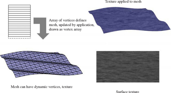
Much of the visible complexity of a mesh object is captured by a surface texture. The texture image may have a regular pattern, making it possible to repeat a small texture over the entire surface. Examples of surfaces with repeating patterns include clouds and water. It is often convenient to use a procedurally generated texture (see Section 18.3) in these cases. This is because the spatial frequency components of a procedural texture can be finely controlled, making it easy to create a texture that wraps across a surface without artifacts.
The texture may be updated dynamically in a number of ways. The direct method is to simply update the texture image itself using subimages. But image updates are expensive consumers of bandwidth. For many applications, lower-cost methods can create a dynamic texture without updating new images. In some cases, simply warping the texture on the surface is sufficient. The texture’s appearance can also be modified by changing the underlying vertex color, rendering with a texture environment such as GL_BLEND or GL_MODULATE. If the texture image itself must be modified, a procedural texture is a good choice for animation, since it is easy to create a series of slowly varying images by varying the input parameters of the generation functions.
We’ll describe dynamic meshes in more depth through a set of application examples. They illustrate the technique in more detail, showing how they can solve problems for particular application areas.
Water
A large body of research has focused on modeling, shading, and reproducing optical effects of water (Watt, 1990; Peachey, 1986; Fournier, 1986), yet most methods still present a large computational burden to achieve a realistic image. Nevertheless, it is possible to borrow from these approaches and achieve reasonable results while retaining interactive performance (Kass, 1990; Ebert, 1994).
Dynamic mesh techniques can provide good realism efficiently enough to maintain interactive frame rates. The dynamics of waves can be simulated using procedural models and rendered using meshes computed from height fields. The mesh vertices are positioned by modulating the height of the vertices with a sinusoid to simulate simple wave patterns, as shown in Figure 18.8. The frequency and amplitude of the waves can be varied to achieve different effects. The phase of the sinusoid can be varied over time to create wave motion.
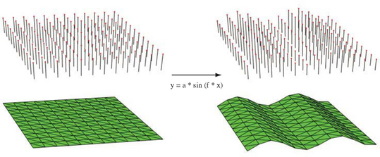
The mesh geometry can be textured using simple procedural texture images, producing a good simulation of water surfaces. Synthetic perturbations to the texture coordinates, as outlined in Section 18.3.7, can also be used to help animate the water surface.
If there is an adequate performance margin, the rendering technique can be further embellished. Multipass or multitexture rendering techniques can be used to layer additional effects such as surf. The reflective properties of the water surface can also be more accurately simulated. Environment mapping can be used to simulate basic reflections from the surface, such as sun smear. This specular reflection can be made more physically accurate using environment mapping that incorporates the Fresnel reflection model described in Section 15.9. The bump-mapping technique described in Section 15.10 can be used to create the illusion of ripples without having to model them in the mesh geometry. The bump maps can be updated dynamically to animate them.
Animating water surface effects also extends to underwater scenes. Optical effects such as caustics can be approximated using OpenGL, as described by Nishita and Nakamae (Nishita, 1994), but interactive frame rates are not likely to be achieved. A more efficient, if less accurate, technique to model such effects uses a caustic texture to modulate the intensity of any geometry that lies below the surface. Other below-surface effects can also be simulated. Movements of the water (surge) can be simulated by perturbing the vertex coordinates of submerged objects, again using sinusoids. Blueish-green fog can be used to simulate light attenuation in water.
Cloud Layers
Cloud layers, in many cases, can be modeled well with dynamic meshes. The best candidates are cloud layers that are continuous and that have distinct upper and lower boundaries. Clouds in general have complex and chaotic boundaries, yet when viewed from a distance or from a viewing angle other than edge-on to the layer boundary this visual complexity is less apparent. In these cases, the dynamic mesh can approximate the cloud layer boundary, with the surface texture supplying the visual complexity. In the simplest case, the dynamic mesh geometry can be simplified to a single quadrilateral covering the sky.
The procedural texture generation techniques described in Section 18.3 can be used to create cloud layer textures. The texture can be a simple luminance image, making it possible to model slowly varying color changes (such as the effect of atmospheric haze) by changing vertex colors in the dynamic mesh. Thin broken cloud layers can also be simulated well if the viewer is not too close to the cloud layer. A luminance cloud texture can be used to blend a white constant texture environment color into a blue sky polygon. If the view is from above the cloud layer, a texture with alpha can be used instead to provide transparency. Rendered with blending or alpha test, the texture can stencil appropriately shaped holes in the mesh polygon, showing the ground below.
Dynamic aspects of cloud layers can also be modeled. Cloud drift can be simulated by translating the textured particles across the sky, along with changes in the mesh geometry, as appropriate.
18.3 Procedural Texture Generation
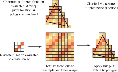
Although many textures are created from natural or synthetic images, textures can also be created by directly evaluating a procedure to generate texel colors. A function is chosen that generates colors as a function of texture coordinates: color = p(s, t, r, q). A procedural texture can be created by evaluating this function at every texel location in a texture image. There is a class of these procedures, known as filtered noise functions, that are particularly useful for generating images for natural features. The images created have similar features at different levels of spatial resolution. This result can be created directly using an appropriate function, or through a multistep process by creating a high-resolution image and then compositing it with scaled and filtered versions of itself. The resulting textures can simulate the appearance of such diverse phenomena as fire, smoke, clouds, and certain types of stone, such as marble. This class of procedural texture, and how it is used in RenderMan shaders, is described in Ebert (1994).
18.3.1 Filtered Noise Functions
Procedural textures can be generated “on the fly,” producing texture color values as needed during the filtering process. Texture images created this way are defined over a continuous range of texture coordinates (using floating-point representations of the input parameters). This method is very powerful, and is the basis for high-quality “shader-based” texturing approaches. It can be accelerated in hardware using fragment programs, but only if the shader hardware is powerful enough to implement the generating function’s algorithm.
Instead of this general method, we’ll use more limited but efficient approach. A pseudorandom image is created in software using a simpler generating function, and is then loaded into a texture map. Texturing is used to convolve and scale the image as necessary to produce the final filtered image. Since the generating function is only evaluated to create a discrete texture image, the generating function need only create valid values at texel locations. This makes it possible to create simpler, discrete versions of the randomizing algorithm, and to make use of a texture-mapping technique to efficiently resample the source images at multiple frequencies. It uses a combination of pseudorandom values, polygon rendering, and texture-filtering techniques to create filtered images.
To create a texture image, the generating function must create color and intensity values at every texel location. To do this efficiently with OpenGL, the algorithms use rectangular grids of values, represented as pixel images. Each 2D grid location is defined to be separated from its neighbors by one unit in each dimension. Both the input and output of the function are defined in terms of this grid. The input to the function is a grid with pseudorandom “noise” values placed in each location. The output is the same grid properly filtered, which can then be used as a component of the final texture image.
The characteristics and distribution of the input noise values, and the filtering method applied to them, determines the characteristics of the final noise function image. A procedural texture must always produce the same output at a given position in the texture, and must produce values limited to a given range. Both of these requirements are met by generating the image once, loading it into a texture map, and mapping it as many times as necessary onto the target geometry.
Another important criterion of procedurally generated textures is that they be band-limited to a maximum spatial frequency of about one. This limit ensures that the filtered image can be properly sampled on the texel grid without aliasing. Any initial set of pseudorandom noise values should therefore be filtered with a low-pass filter at this maximum spatial frequency before use in a texture.
Figure 18.9 illustrates the steps in producing a filtered noise function. The direct approach is simple: a continuous function is written that outputs filtered color values as a function of surface position. It is used during the rasterization phase to set the pixel colors of the polygon. The texture approach requires more steps. A discrete function is used to generate an unfiltered image. The image is filtered and resampled over one or more frequencies using texture mapping. The resulting image is then applied to the geometry as a texture.
The initial noise inputs need to be positioned in the image before filtering. Their distribution affects the appearance of the resulting image. One common method is to distribute the initial values in a uniform grid. Textures that start from a regular grid of noise values are called lattice noise functions. Lattice noise is simple to create, but can exhibit axis-aligned artifacts. The noise functions can also be distributed in a nonuniform stochastic pattern, avoiding this problem. In the literature, this technique is called a sparse convolution. Another method designed to avoid the artifact problem is called spot noise, described by van Wijk (1991). To use image-based filtering techniques, nonuniform spacing is allowed, but all random data must be placed on a grid point.
How the filtering step is applied to the input noise can vary (Ebert, 1994). Two common filters interpolate lattice noise values in quite different ways. In value noise, the filter function directly interpolates the value of the random noise data placed at all lattice points. In gradient noise, noise data is used to produce vector values at each lattice point, which are then interpolated to produce filtered values. A frequency analysis of gradient noise shows no contribution at a frequency of zero. This is useful because it makes it easy to composite multiple noise functions without introducing a bias term.
Simple noise functions are often combined to create more complex ones. A common case is a function composed of scaled versions of the output of the original function. The scaling is done so that the output frequency is lower by a power-of-two: 2, 4, 8, and so on. These lower-frequency derivative functions are called the octaves of the original function. The octaves are composited with the original version of the noise function. The compositing step scales the output of each function by a set of weighting factors, which can be varied to produce different effects. The result is a band-limited function that has the appearance of controlled randomness in each frequency band. This distribution of energy in the frequency domain is very similar to random phenomena found in nature, and accounts for the realism of these textures.
18.3.2 Generating Noise Functions
A discrete version of the generating function described previously can be created in the framebuffer using OpenGL. The generation algorithm must be able to start with a grid of random values, stretch them so that each covers a larger area (to create lower-frequency octaves), and apply low-pass filtering (essentially blending them).
One simple way to do this is to create a texture composed of random values at each texel, and then stretch and interpolate the values by rendering a textured rectangle. The rectangle could be textured using bilinear filtering, and drawn at an appropriate size to create the desired octave. Bilinear interpolation, however, is a poor filter for this application. This is especially true when creating lower-frequency octaves, where random values must be interpolated across a large area.
Some OpenGL implementations support better texture-filtering modes, such as bicubic filtering, which may produce results of acceptable quality. Some implementations of bicubic filtering may have limited subtexel precision, however, causing noticeable banding when creating lower-frequency octaves. Both bilinear and bicubic filters also have the limitation that they can only interpolate existing values. This limits the noise filter to produce only value noise; the approach isn’t flexible enough to work with gradient noise. A more powerful approach is to spread each value across the image using convolution techniques. Fortunately, this method can be made efficient with a clever application of texture mapping.
18.3.3 Filtering Using Texture Convolution
Instead of simply creating textures of random values and stretching them to create filtered octaves using built-in texture filtering, the octave images can be created using a convolution approach. A convolution filter can apply the appropriate filtering to each random value as needed. Filter kernels that cover a larger area can be used to create lower-frequency octaves. Convolution is discussed in Section 12.6. The approach shown here accelerates convolution by encoding the convolution filter into a texture image. A rectangle, whose color is the random value to be convolved, is rendered with the monochrome texture containing the convolution filter image applied to it.
To illustrate, consider a low-pass filtering operation on an image. The input image can be thought of as a grid of values. To low-pass filter the image, the values at each grid location must be blended with their neighbors. The number of neighboring values that are blended is called the filter’s extent or support (Section 4.3); it defines the width of the filter. Blending the value of location i, j with a neighbor at i + n, j + m can be expressed as valuei+n,j+m = valuei+n,j+m * filter + valuei,j * (1 − filter). The filter function controls the contribution location i, j makes to each of its neighbors. The extent of the filter and its values determine the filtering effect. In general, the wider the extent (i.e., the more neighbors affected), the lower the maximum frequency a low-pass filter can achieve and the more work required to apply the filtering (because it requires operating on more values).
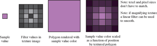
The convolution operation can be implemented using a combination of texturing and blending. A texture map is created that represents a convolution kernel, containing the desired filter weights for each texel neighbor. The size of the filter texels doesn’t have to be one-to-one with the destination pixels. The resolution of the texture filter is determined by the complexity of the filtering function. A simple linear filtering function can be represented with a small texture, since OpenGL’s linear magnification can be used to interpolate between filter values. The filter texels can modulate a sample value by using the filter texture to texture a rectangle colored with the sample. If the texture environment is GL_MODULATE, a single component GL_LUMINANCE texture containing the filter function will scale the base color by the texel values. The texture performs two functions: it spreads the sample value over the region of the rectangle and modulates the sample value at the resolution of the filter texture. Rendering the textured rectangle updates the values in the framebuffer with the filtered values for a single sample, as shown in Figure 18.10.
A straightforward filtering pass based on this idea reads each sample value and uses it to color a texture rectangle modulated by the filter texture. The process is repeated, shifting the textured rectangle and substituting a new sample value for the rectangle color for each iteration. The filtered results for each sample are combined using blending, or for higher color resolution using the accumulation buffer.
The following is a very simple example of this approach in more detail. It starts with a 512×512 grid of sample values and applies a 2×2 box filter. The filter spreads the sample, considered to be at the lower-left corner of the filter, over a 4×4 region.
1. Create a 2×2 luminance filter, each value containing the value .25.
2. Configure the transform pipeline so that object coordinates are in screen space.
3. Clear a 512×512 region of the framebuffer that will contain the filtered image to black.
4. Create a 512×512 grid of sample values to be filtered.
5. Enable blending, setting the blend function to GL_ONE, GL_ONE.
6. Set the texture environment to GL_MODULATE.
There are a number of parameters that need to be adjusted properly to get the desired filtering. The transformation pipeline should be configured so that the object coordinate system matches screen coordinates. The region of the framebuffer rendered should be large enough to create the filtered image at the desired resolution. The textured rectangle should be sized to cover all neighboring pixels needed to get the desired filtering effect. The resolution of the filter texture itself should be sufficient to represent the filter function accurately for the given rectangle size. The rectangle should be adjusted in x and y to match the grid sample being filtered. The filter marches across the image, one pixel at a time, until the filtering is completed. To avoid artifacts at the edges of the image, the filter function should extend beyond the bounds of the image, just as it does for normal convolution operations. The relationship between sample value and filter function will determine the details of how overlaps should be handled, either by clamping or by wrapping.
Although efficient, there are limitations to this approach. The most serious is the limited range of color values for both the filter texture and the framebuffer. Both the filter function and sample color are limited to the range [0, 1]. This makes it impossible to use filter kernels with negative elements without scaling and biasing the values to keep them within the supported range, as described in Section 14.13.1. Since the results of each filtering pass are accumulated, filters should be chosen that don’t cause pixel color overflow or underflow. Texturing and/or framebuffers with extended range can mitigate these restrictions.
18.3.4 Optimizing the Convolution Process
Although texture mapping efficiently applies the filtered values of a sample point over a large number of pixels, the filtering operation can become expensive since it has to be repeated for every sample in the target image. This process can be optimized, particularly for filters with a small extent, using the following observation. Since a texture map is used to apply a filter function, the filter’s extent can be represented as a rectangular region with a given width and height. Note that two sample values won’t blend with each other during filtering if they are as far apart as the filter’s extent. This independence can be used to reduce the number of passes required to filter an image. Instead of filtering only a single sample value per pass, and iterating over the entire image, the texture filter can be tiled over the entire image at once, reducing the number of passes. If a filter extent is of width w and height h, every w + 1th sample in the horizontal direction and every h + 1th sample in the vertical direction can be filtered at the same time, since they don’t interact with each other.
For a concrete illustration, consider the 2×2 filter with the 4×4 extent in the previous example. For any given sample at i, j, the samples at i + 4, j and i, j + 4 won’t be affected by the sample value at i, j. This means the samples at i + 4, j and i, j + 4 can be filtered at the same time that i, j is sampled by applying three nonoverlapping textured rectangles, each with a different one of the three sample values. Taking full advantage of this idea, the entire image can be tiled with texture rectangles, filtering the samples at i + 4 *n, j + 4 *m. With this technique, the entire image can be filtered in 16 passes. In general, the number of passes required will be equal to the extent of the filter. With this technique, that equals the number of pixels covered by the filter rectangle.
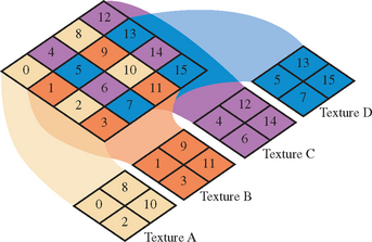
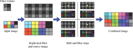
The implementation of this technique can be further streamlined. The tiled set of textured rectangles, each colored with a different sample value, is replaced with a single rectangle textured with two textures. The first texture is the filter texture, with the wrap parameter set to GL_REPEAT and texture coordinates set so that it tiles over the entire rectangle, creating filters of the same size as the original technique. The second texture contains the sample values themselves. It is composed of a subset of the grid sample points that satisfies the i + 4n, j + 4m equation, as illustrated in Figure 18.11. In a two-pass technique (or single pass if multitexturing is available), the sample-points texture can be modulated by the filter texture, creating a sparse grid of filtered values in a single texturing pass. The process can be repeated with the same filter texture, and offset sample textures, such as i + 1 + 4n, j + 4m and i + 4n, j + 1 + 4m. The large rectangle should be offset to match the offset sample values, as shown in Figure 18.12. The process is repeated until every sample in the filter’s extent has been computed.
The example steps that follow illustrate the technique in more detail. It assumes that multitexturing is available. Two textures are used: the filter texture, consisting a single component texture containing values that represent the desired filter function, and the sample texture, containing the sample values to be filtered.
1. Set a blending function to combine the results from rendering passes or configure the accumulation buffer.
2. Choose a rectangle size that covers the destination image.
3. Create the sample texture from a subset of the samples, as described previously. Bind it to the first texture unit.
4. Scale the texture coordinates of the sample texture so that each sample matches the desired extent of the filter.
5. Bind the second texture unit to the filter texture.
6. Set the wrap mode used on the filter texture to GL_REPEAT.
7. Scale the texture coordinates used on the filter texture so it has the desired extent.
8. Set the texture environment mode so that the filter texture scales the intensity of the sample texture’s texels.
9. Render the rectangle with the two textures enabled.
10. If using the accumulation buffer, accumulate the result.
11. This is one pass of the filtering operation. One sample has been filtered over the entire image. To filter the other samples:
(a) Shift the position of the rectangle by one pixel.
(b) Update the sample texture to represent the set of samples that matches the new rectangle position.
(c) Rerender the rectangle, blending with the old image, or if using the accumulation buffer make an accumulation pass.
(d) Repeat until each sample in the filter’s extent has been processed.
The subset of the sample grid can be efficiently selected by rendering a texture with the sample values, using GL_NEAREST for the minification filter. By rendering a rectangle the size of the reduced sample grid, and setting the texture coordinates to minify and bias the texture appropriately, the minification filter can be used to only render the samples desired.
The position of the rectangle, the way the filter and sample textures are positioned on the rectangle, and the grid samples used in each pass are determined by the relationship between the sample point and the filter. The filter is considered to have a sample position, which describes the position of the input sample relative to the filter. This position is needed to properly position the filter relative to the input samples as each subset of samples is filtered. Many filters assume that the input sample is at the center of the filter. This can’t always be done, as there is no center for a filter with a width and/or height that is even. To get the edges of the filtered image correct, the textured rectangle can overlap beyond the edge of the image.
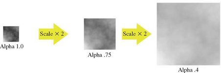
Creating Octaves
Once a filtered noise image is created, it is a simple matter to create lower octaves. The original image being filtered has a maximum spatial frequency component. Simply scaling the size of the textured rectangle, in the approach described previously, will change the filter extent and create a filtered image with different frequency components. Doubling the size of the textured rectangle, for example, will create an image with frequency components that are one-half the original. If the rectangle is to be increased in size, be sure that the filter texture has sufficient resolution to represent the filter accurately when spread over a larger number of pixels.
18.3.5 Spectral Synthesis
Using the previous algorithm, multiple octaves can be created and combined to create multispectral images. The process of rescaling the filter size can be streamlined by changing the texture coordinates in the texture transform matrix. The matrix also makes it easy to translate and scale texture coordinates. Translating texture coordinates by a random factor for each octave prevents the samples near the texture coordinate origin from aligning. Such alignment can lead to noticeable artifacts.
Natural phenomena often have a frequency spectrum where lower-frequency components are stronger. Often the amplitude of a particular frequency is proportional to ![]() . To replicate this phenomenon, the intensity of each octave’s filtered samples can be scaled. An easy way to do this is to apply a frequency-dependent scale factor when coloring the textured rectangles.
. To replicate this phenomenon, the intensity of each octave’s filtered samples can be scaled. An easy way to do this is to apply a frequency-dependent scale factor when coloring the textured rectangles.
Just as each filtered sample must be blended with its neighbors within the filter’s extent, so each scaled octave must be blended with the others to create a multispectral texture. As with the original filtering method, blending can be done in the framebuffer, or if more color precision is needed using the accumulation buffer. If desired, the weighting factors for each octave can be applied when the octaves are blended, instead of when the filter rectangle is shaded. The steps that follow use the technique for creating a filtered image mentioned previously to generate and combine octaves of that image to produce a multispectral texture map.
1. Create the original filtered image using the filtered noise technique described previously.
2. For each octave (halving the previous frequency):
(a) Create a sample texture with one quarter the samples of the previous level.
(b) Halve the texture coordinate scale used to texture the rectangle. This will quadruple the extent of each filtered sample.
(c) Draw textured rectangles to filter the image with both textures. The number of rendering steps must be quadrupled, since each filtered sample is covering four times as many pixels.
(d) Scale the intensity of the resulting image as needed.
(e) Combine the new octave with the previous one by blending or using the accumulation buffer.
Generalizing the Filtering Operation
Gradient noise can be also created using the previous method. Instead of an averaging filter, a gradient filter is used. Since a gradient filter has both positive and negative components, multiple passes are required, segmenting the filter into positive and negative components and changing the blend equation to create the operation desired.
Since texture coordinates are not restricted to integral values, the texture filter can be positioned arbitrarily. This makes it possible to generalize the previous technique to create noise that is not aligned on a lattice. To create nonaligned noise images, such as sparse convolution noise (Lewis, 1989) or spot noise (van Wijk, 1991), filter the sample values individually, randomly positioning the filter texture. Instead of drawing the entire point-sampled texture at once, draw one texel and one copy of the filter at a time for each random location. This is just a generalization of the initial texture approach described previously in Section 18.3.3.
18.3.6 Turbulence
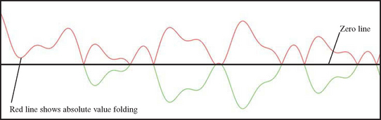
A variation of the process used to create noise textures can create images that suggest turbulent flow. To create this type of image, first-derivative (slope) discontinuities are introduced into the noise function. A convenient way to do this on a function that has both positive and negative components is to take its absolute value. Although OpenGL does not include an absolute value operator for framebuffer content in the fixed-function pipeline, the same effect can be achieved using the accumulation buffer.
The accumulation buffer can store signed values. Unsigned values from the framebuffer, in the range [0, 1], can be stretched to range [−1, 1] using GL_ADD and GL_MULT operations in the accumulation buffer. The absolute value of the stretched function can be obtained by reading back from the accumulation buffer; returned values are clamped to be positive. The negative values are returned using a scale factor of − 1. This flips the negative components to positive, which will survive clamping during the return. The result is the absolute value of the stretched image. The discontinuity will appear at the midway values, one-half of the original function (see Figure 18.13).
The following steps illustrate the details of this technique. They would be applied to a filtered image in the framebuffer.
1. Load the accumulation buffer using glAccum(GL_LOAD,1.0).
2. Bias the image in the buffer by 1/2 using glAccum(GL_ADD,-0.5), making it signed.
3. Scale the image by 2 using glAccum(GL_MULT,2.0), filling the [−1, 1] range.
4. Return the image using glAccum(GL_RETURN,1.0), implicitly clamping to positive values.
5. Save the image in the color buffer to a texture, application memory, or other color buffer.
6. Return the negative values by inverting them using glAccum(GL_RETURN,-1.0).
7. Set the blend function to GL_ONE for both source and destination.
8. Draw the saved image from step 5 onto the image returned from the accumulation buffer. The blend mode will combine them.
The color buffer needs to be saved after the first GL_RETURN because the second GL_RETURN will overwrite the color buffer. OpenGL does not define blending for accumulation buffer return operations. One way to implement this is using both the front and back color buffers in a double-buffered framebuffer.
18.3.7 Random Image Warping
A useful application for a 2D noise texture is to use the noise values to offset texture coordinates. Texture coordinates are applied with regular spacing to a triangle mesh. The noise values are used to displace each texture coordinate. If the grid and its texture coordinates are then textured with an image, the resulting image will be distorted, creating a somewhat painterly view of the image. A more severe distortion can be created by using the noise values directly as texture coordinates, rather than as offsets.
By setting the proper transforms, the process of using noise values as texture coordinates can be automated. Capturing the noise image into a vertex array as texture coordinates, and setting the texture transform matrix appropriately, makes it possible to render the texture with the noise image texture coordinates directly. A variation of this technique, where the noise values are used as vertex positions in the vertex array and then transformed by the appropriate modelview matrix, makes it possible to use noise values as vertex positions.
Another similar use of a 2D noise texture is to distort the reflection of an image. In OpenGL, reflections on a flat surface can be done by reflecting a scene across the surface. The results are copied from the framebuffer to texture memory, and in turn drawn with distorted texture coordinates. The shape and form of the distortion are controlled by modulating or attenuating the contents of the framebuffer after the noise texture is drawn but before it is copied to texture memory. This can produce interesting effects such as water ripples.
18.3.8 Generating 3D Noise
Noise images are not limited to two dimensions. 3D noise images can also be synthesized using the techniques described here. To do this correctly requires a 3D filter instead of a 2D one. In the 2D case, a 2D filter is created by converting a 2D filter function into a texture image, then using the texture to modulate an input color. For 3D filtering, the same apporach can be used. A discrete 3D filter is created from a 3D filter function, then stored in a 3D texture. Using a 3D texture filter to create a 3D noise image requires slicing the 3D block of pixels into 2D layers, a technique similar to the volume visualization techniques discussed in Section 20.5.8. As with volume visualization, 3D texturing is done using multiple textured 2D slices, building up a 3D volume one layer at a time. Like volume visualization, it also can be done using true 3D textures, or a series of 2D textures applied in layers instead.
As with 2D noise filtering, it can be clearer to consider the simple brute-force case for 3D. A 3D grid of random values is created with the desired resolution. A 3D filter texture is created, either as a single 3D texture or as a series of 2D textures, each representing a different r coordinate in the 3D texture. As with 2D textures, the 3D filter function has an extent, but this time it is measured in three dimensions. As with 2D, a rectangle is rendered, sized to match the extent of the texture filter and sized to cover the pixels that should be modified by the filter. Unlike the 2D case, a series of rectangles must be drawn, spanning the layers of the image covered by the filter’s extent. The rendering process is repeated, shifting the texture rectangles as necessary and iterating through the samples in the 3D sample grid. As with the 2D case, the rectangle is shifted to align the filter texture properly as each new grid value is filtered. In the 3D case, the image layers the rectangles are applied must also be shifted.
Since 3D framebuffers are not supported in OpenGL, one or more 2D framebuffers must be segmented into layers to provide rendering surfaces representing the layers in the 3D noise image. If there is sufficient space in a single framebuffer, the framebuffer can be split up into a grid of rectangular regions, each representing a different layer. The application managing the layers maps a different framebuffer region to each layer. Multiple framebuffers may be necessary to provide enough pixels to represent all of the layers in the noise image. Once the filtered image layers have all been rendered, the results can be copied into a single 3D noise texture, or loaded into a series of 2D textures, depending on the requirements of the application.
As with the 2D case, the procedure can be optimized, wrapping the filter texture in 3 dimensions, and filtering multiple samples (that aren’t under the same filter’s extent) at once. The samples themselves can be assembled into a 3D sample texture, or a series of 2D sample textures can be used. Like the 2D technique, the texture coordinates of the sample texture are scaled so that each sample matches the extent of its filter function. As before, the filter texture is used to spread and modulate the sample texture’s values onto the framebuffer regions. The 3D case requires this process to be applied to multiple layers.
To synthesize a 3D function with different frequencies, first create a 3D noise image for each frequency and composite a weighted set of frequencies, as was done in the 2D case. A large amount of memory is required to store the different 3D noise functions. Many implementations severely restrict the maximum size of 3D textures, so an application should query to see if the implementation’s available resolutions are sufficient for the application.
Generating 2D Noise to Simulate 3D Noise
Creating 3D noise function can be computationally expensive. The resulting textures are large consumers of texture and system memory. In some cases, clever use of 2D noise functions can sometimes successfully substitute for true 3D noise functions. To make 2D noise functions adequately approximate the appearance of a true 3D noise function, the 2D function should match the appearance of the 3D function when it is applied to the target surface. The texture image must be updated if the target geometry changes. This makes “pseudo-3D” noise textures less general.
Pseudo-3D noise textures are simple to implement if the original noise function uses spot noise (van Wijk, 1991). The pseudo-3D noise function is designed around the geometry it will texture. Spots are still created in 3D space, but only spots that are close enough to the geometry surface to make a contribution to the final 2D noise image are used. Once the proper spots are selected, they are rendered onto the 2D surface so that at each fragment the value of the spot is determined by the object-space distance from the center of the spot to that fragment.
Depending on the complexity of the geometry, it may be possible to make an acceptable approximation to the correct spot value by distorting a 2D spot texture. One possible way to improve the approximation is to compensate for a nonuniform mapping of the noise texture to the geometry. Van Wijk describes how he does this by nonuniformly scaling a spot. Approximating the correct spot value is most important when generating the lower octaves, where the spots are largest and errors are most noticeable.
Trade-offs Between True and Simulated 3D Noise
When choosing between a true 3D noise texture and a simulation of one, the most accurate approach is to use the 3D one. Per-frame overhead may also be lower for true 3D textures. They can be used with arbitrary geometry without reloading the texture image (assuming the OpenGL implementation supports 3D textures). 3D noise textures suffer the same drawbacks as any 3D texture technique. Generating a 3D noise texture requires a large amount of memory and a large number of passes, especially if the filter convolves a large number of input values at a time. If memory resources are constrained, the 2D approximation can work well on a useful class of geometry. The 2D texture doesn’t require nearly as many passes to create, but it does require knowledge of the geometry and additional computation in order to properly shape the spot.
18.4 Summary
This chapter described some classes of advanced techniques useful for simulating natural phenom ena. The ideas are general and serve as building blocks for modeling a variety of natural phenom ena. Reproducing the appearance of objects in nature continues to be an area of considerable activity. The addition of vertex and fragm ent programs to the OpenGL pipeline significantly increases the range of processes that can be modeled directly in the pipeline and will serve as a catalyst for numerous new techniques.
1Added as a core feature in OpenGL 1.4.