Topics can be useful on their own to build small vignettes with words that are in the previous screenshot. These visualizations could be used to navigate a large collection of documents and, in fact, they have been used in just this way.

However, topics are often just an intermediate tool to another end. Now that we have an estimate for each document about how much of that document comes from each topic, we can compare the documents in topic space. This simply means that instead of comparing word per word, we say that two documents are similar if they talk about the same topics.

This can be very powerful, as two text documents that share a few words may actually refer to the same topic. They may just refer to it using different constructions (for example, one may say the President of the United States while the other will use the name Barack Obama).

At this point, we can redo the exercise we performed in the previous chapter and look for the most similar post, but by using the topics. Whereas previously we compared two documents by comparing their word vectors, we can now compare two documents by comparing their topic vectors.

For this, we are going to project the documents to the topic space. That is, we want to have a vector of topics that summarizes the document. Since the number of topics (100) is smaller than the number of possible words, we have reduced dimensionality. How to perform these types of dimensionality reduction in general is an important task in itself, and we have a chapter entirely devoted to this task. One additional computational advantage is that it is much faster to compare 100 vectors of topic weights than vectors of the size of the vocabulary (which will contain thousands of terms).

Using gensim, we saw before how to compute the topics corresponding to all documents in the corpus:

  >>> topics = [model[c] for c in corpus]
  >>> print topics[0]
[(3, 0.023607255776894751),
  (13, 0.11679936618551275),
  (19, 0.075935855202707139),
  (92, 0.10781541687001292)]

We will store all these topic counts in NumPy arrays and compute all pairwise distances:

>>> dense = np.zeros( (len(topics), 100), float)
  >>> for ti,t in enumerate(topics):
  …    for tj,v in t:
  …      dense[ti,tj] = v

Now, dense is a matrix of topics. We can use the pdist function in SciPy to compute all pairwise distances. That is, with a single function call, we compute all the values of sum((dense[ti] – dense[tj])**2):

>>> from scipy.spatial import distance
>>> pairwise = distance.squareform(distance.pdist(dense))

Now we employ one last little trick; we set the diagonal elements of the distance matrix to a high value (it just needs to be larger than the other values in the matrix):

>>> largest = pairwise.max()
  >>> for ti in range(len(topics)):
    pairwise[ti,ti] = largest+1

And we are done! For each document, we can look up the closest element easily:

  >>> def closest_to(doc_id):
    return pairwise[doc_id].argmin()

For example, here is the second document in the collection (the first document is very uninteresting, as the system returns a post stating that it is the most similar):

From: [email protected] (Gordon Banks)
Subject: Re: request for information on "essential tremor" and Indrol?
In article <[email protected]> [email protected] writes:
Essential tremor is a progressive hereditary tremor that gets worse when the patient tries to use the effected member. All limbs, vocal cords, and head can be involved.  Inderal is a beta-blocker and is usually effective in diminishing the tremor. Alcohol and mysoline are also effective, but alcohol is too toxic to use as a treatment.
----------------------------------------------------------------Gordon Banks  N3JXP      | "Skepticism is the chastity of the intellect, and
[email protected]   |  it is shameful to surrender it too soon."
  ----------------------------------------------------------------

If we ask for the most similar document, closest_to(1), we receive the following document:

From: [email protected] (Gordon Banks)
Subject: Re: High Prolactin

In article <[email protected]> [email protected] (John E. Rodway) writes:
>Any comments on the use of the drug Parlodel for high prolactin in the blood?
>It can suppress secretion of prolactin.  Is useful in cases of galactorrhea. Some adenomas of the pituitary secret too much.
------------------------------------------------------------------
Gordon Banks  N3JXP      | "Skepticism is the chastity of the intellect, and [email protected]   |  it is shameful to surrender it too soon."
  ----------------------------------------------------------------

We received a post by the same author discussing medications.

Modeling the whole of Wikipedia

While the initial LDA implementations could be slow, modern systems can work with very large collections of data. Following the documentation of gensim, we are going to build a topic model for the whole of the English language Wikipedia. This takes hours, but can be done even with a machine that is not too powerful. With a cluster of machines, we could make it go much faster, but we will look at that sort of processing in a later chapter.

First we download the whole Wikipedia dump from http://dumps.wikimedia.org. This is a large file (currently just over 9 GB), so it may take a while, unless your Internet connection is very fast. Then, we will index it with a gensim tool:

python -m gensim.scripts.make_wiki enwiki-latest-pages-articles.xml.bz2 wiki_en_output

Run the previous command on the command line, not on the Python shell. After a few hours, the indexing will be finished. Finally, we can build the final topic model. This step looks exactly like what we did for the small AP dataset. We first import a few packages:

>>> import logging, gensim
>>> logging.basicConfig(
    format='%(asctime)s : %(levelname)s : %(message)s',
    level=logging.INFO)

Now, we load the data that has been preprocessed:

>>> id2word = gensim.corpora.Dictionary.load_from_text('wiki_en_output_wordids.txt')
>>> mm = gensim.corpora.MmCorpus('wiki_en_output_tfidf.mm')

Finally, we build the LDA model as before:

>>> model = gensim.models.ldamodel.LdaModel(
    corpus=mm,
    id2word=id2word,
    num_topics=100,
    update_every=1,
    chunksize=10000,
    passes=1)

This will again take a couple of hours (you will see the progress on your console, which can give you an indication of how long you still have to wait). Once it is done, you can save it to a file so you don't have to redo it all the time:

  >>> model.save('wiki_lda.pkl')

If you exit your session and come back later, you can load the model again with:

  >>> model = gensim.models.ldamodel.LdaModel.load('wiki_lda.pkl')

Let us explore some topics:

  >>> topics = []
  >>> for doc in mm:
      topics.append(model[doc])

We can see that this is still a sparse model even if we have many more documents than before (over 4 million as we are writing this):

  >>> import numpy as np
  >>> lens = np.array([len(t) for t in  topics])
  >>> print np.mean(lens)
  6.55842326445
  >>> print np.mean(lens <= 10)
  0.932382190219

So, the average document mentions 6.5 topics and 93 percent of them mention 10 or fewer.

Note

If you have not seen the idiom before, it may be odd to take the mean of a comparison, but it is a direct way to compute a fraction.

np.mean(lens <= 10) is taking the mean of an array of Booleans. The Booleans get interpreted as 0s and 1s in a numeric context. Therefore, the result is a number between 0 and 1, which is the fraction of ones. In this case, it is the fraction of elements of lens, which are less than or equal to 10.

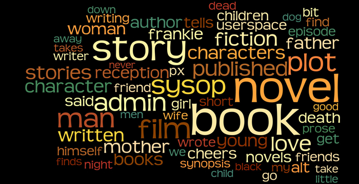
We can also ask what the most talked about topic in Wikipedia is. We first collect some statistics on topic usage:

  >>> counts = np.zeros(100)
  >>> for doc_top in topics:
  …    for ti,_ in doc_top:
  …      counts[ti] += 1
  >>> words = model.show_topic(counts.argmax(), 64)

Using the same tool as before to build up visualization, we can see that the most talked about topic is fiction and stories, both as books and movies. For variety, we chose a different color scheme. A full 25 percent of Wikipedia pages are partially related to this topic (or alternatively, 5 percent of the words come from this topic):

Note

These plots and numbers were obtained when the book was being written in early 2013. As Wikipedia keeps changing, your results will be different. We expect that the trends will be similar, but the details may vary. Particularly, the least relevant topic is subject to change, while a topic similar to the previous topic is likely to be still high on the list (even if not as the most important).

Alternatively, we can look at the least talked about topic:

  >>> words = model.show_topic(counts.argmin(), 64)

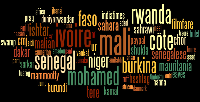
The least talked about are the former French colonies in Central Africa. Just 1.5 percent of documents touch upon it, and it represents 0.08 percent of the words. Probably if we had performed this exercise using the French Wikipedia, we would have obtained a very different result.