At its core, Naive Bayes classification is nothing more than keeping track of which feature gives evidence to which class. To ease our understanding, let us assume the following meanings for the variables that we will use to explain Naive Bayes:

Variable	Possible values	Meaning
	"pos", "neg"	Class of a tweet (positive or negative)
	Non-negative integers	Counting the occurrence of awesome in the tweet
	Non-negative integers	Counting the occurrence of crazy in the tweet

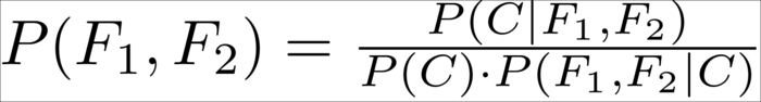
During training, we learn the Naive Bayes model, which is the probability for a class when we already know features and . This probability is written as .

Since we cannot estimate this directly, we apply a trick, which was found out by Bayes:

If we substitute with the probability of both features and occurring and think of as being our class , we arrive at the relationship that helps us to later retrieve the probability for the data instance belonging to the specified class:

This allows us to express by means of the other probabilities:

We could also say that:

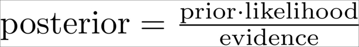
The prior and evidence values are easily determined:

From the probability theory, we also know the following relationship:

This alone, however, does not help much, since we treat one difficult problem (estimating ) with another one (estimating ).

However, if we naively assume that and are independent from each other, simplifies to and we can write it as follows:

Putting everything together, we get this quite manageable formula:

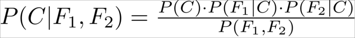
The interesting thing is that although it is not theoretically correct to simply tweak our assumptions when we are in the mood to do so, in this case it proves to work astonishingly well in real-world applications.

Given a new tweet, the only part left is to simply calculate the probabilities:

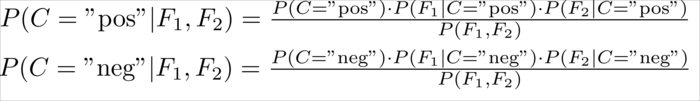
We also need to choose the class having the higher probability. As for both classes the denominator, , is the same, so we can simply ignore it without changing the winner class.

Note, however, that we don't calculate any real probabilities any more. Instead, we are estimating which class is more likely given the evidence. This is another reason why Naive Bayes is so robust: it is not so much interested in the real probabilities, but only in the information which class is more likely to. In short, we can write it as follows:

Here we are calculating the part after argmax for all classes of C ("pos" and "neg" in our case) and returning the class that results in the highest value.

But for the following example, let us stick to real probabilities and do some calculations to see how Naive Bayes works. For the sake of simplicity, we will assume that Twitter allows only for the two words mentioned earlier, awesome and crazy, and that we had already manually classified a handful of tweets:

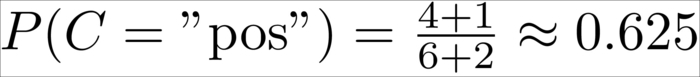
In this case, we have six total tweets, out of which four are positive and two negative, which results in the following priors:

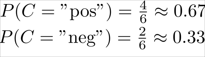
This means, without knowing anything about the tweet itself, we would be wise in assuming the tweet to be positive.

The piece that is still missing is the calculation of and , which are the probabilities for the two features and conditioned on class C.

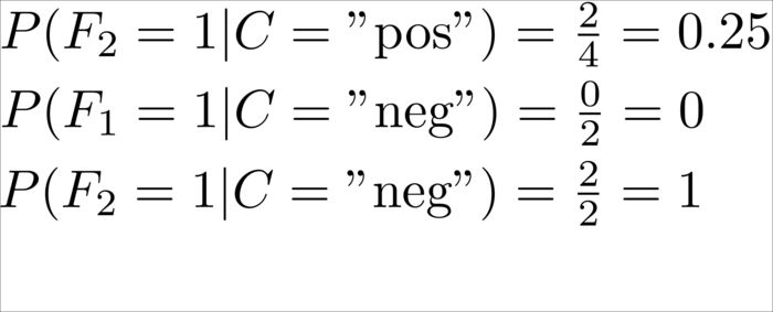
This is calculated as the number of tweets in which we have seen that the concrete feature is divided by the number of tweets that have been labeled with the class of . Let's say we want to know the probability of seeing awesome occurring once in a tweet knowing that its class is "positive"; we would have the following:

Since out of the four positive tweets three contained the word awesome, obviously the probability for not having awesome in a positive tweet is its inverse as we have seen only tweets with the counts 0 or 1:

Similarly for the rest (omitting the case that a word is not occurring in a tweet):

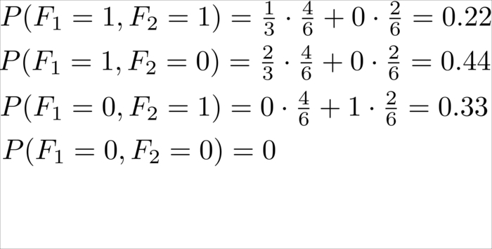
For the sake of completeness, we will also compute the evidence so that we can see real probabilities in the following example tweets. For two concrete values of and ,we can calculate the evidence as follows:

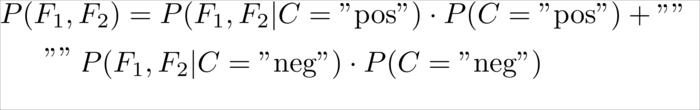
This denotation "" leads to the following values:

Now we have all the data to classify new tweets. The only work left is to parse the tweet and give features to it.

Tweet			Class probabilities	Classification
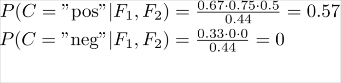
awesome	1	0		Positive
crazy	0	1		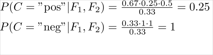Negative
awesome crazy	1	1		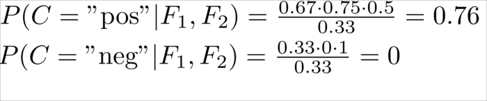Positive
awesome text	0	0		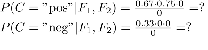Undefined, because we have never seen these words in this tweet before

So far, so good. The classification of trivial tweets makes sense except for the last one, which results in a division by zero. How can we handle that?

When we calculated the preceding probabilities, we actually cheated ourselves. We were not calculating the real probabilities, but only rough approximations by means of the fractions. We assumed that the training corpus would tell us the whole truth about the real probabilities. It did not. A corpus of only six tweets obviously cannot give us all the information about every tweet that has ever been written. For example, there certainly are tweets containing the word "text", it is just that we have never seen them. Apparently, our approximation is very rough, so we should account for that. This is often done in practice with "add-one smoothing".

It is a very simple technique, simply adding one to all counts. It has the underlying assumption that even if we have not seen a given word in the whole corpus, there is still a chance that our sample of tweets happened to not include that word. So, with add-one smoothing we pretend that we have seen every occurrence once more than we actually did. That means that instead of calculating the following:

We now calculate:

Why do we add 2 in the denominator? We have to make sure that the end result is again a probability. Therefore, we have to normalize the counts so that all probabilities sum up to one. As in our current dataset awesome, can occur either zero or one time, we have two cases. And indeed, we get 1 as the total probability:

Similarly, we do this for the prior probabilities:

There is yet another roadblock. In reality, we work with probabilities much smaller than the ones we have dealt with in the toy example. In reality, we also have more than two features, which we multiply with each other. This will quickly lead to the point where the accuracy provided by NumPy does not suffice anymore:

>>> import numpy as np
>>> np.set_printoptions(precision=20) # tell numpy to print out more digits (default is 8)
>>> np.array([2.48E-324])
array([ 4.94065645841246544177e-324]) 
>>> np.array([2.47E-324])
array([ 0.])

So, how probable is it that we will ever hit a number like 2.47E-324? To answer this, we just have to imagine a likelihood for the conditional probabilities of 0.0001 and then multiply 65 of them together (meaning that we have 65 low probable feature values) and you've been hit by the arithmetic underflow:

>>> x=0.00001
>>> x**64 # still fine
1e-320
>>> x**65 # ouch
0.0

A float in Python is typically implemented using double in C. To find out whether it is the case for your platform, you can check it as follows:

>>> import sys
>>> sys.float_info
sys.float_info(max=1.7976931348623157e+308, max_exp=1024, max_10_exp=308, min=2.2250738585072014e-308, min_exp=-1021, min_10_exp=-307, dig=15, mant_dig=53, epsilon=2.220446049250313e-16, radix=2, rounds=1)

To mitigate this, you could switch to math libraries such as mpmath (http://code.google.com/p/mpmath/) that allow arbitrary accuracy. However, they are not fast enough to work as a NumPy replacement.

Fortunately, there is a better way to take care of this, and it has to do with a nice relationship that we maybe still know from school:

If we apply it to our case, we get the following:

As the probabilities are in the interval between 0 and 1, the log of the probabilities lies in the interval -∞ and 0. Don't get irritated with that. Higher numbers are still a stronger indicator for the correct class—it is only that they are negative now.

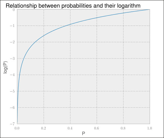
There is one caveat though: we actually don't have log in the formula's nominator (the part preceding the fraction). We only have the product of the probabilities. In our case, luckily we are not interested in the actual value of the probabilities. We simply want to know which class has the highest posterior probability. We are lucky because if we find this:

Then we also have the following:

A quick look at the previous graph shows that the curve never goes down when we go from left to right. In short, applying the logarithm does not change the highest value. So, let us stick this into the formula we used earlier:

We will use this to retrieve the formula for two features that will give us the best class for real-world data that we will see in practice:

Of course, we will not be very successful with only two features, so let us rewrite it to allow the arbitrary number of features:

There we are, ready to use our first classifier from the scikit-learn toolkit.