One of the interesting conclusions from the Netflix Challenge was one of those obvious-in-hindsight ideas: we can learn a lot about you just from knowing which movies you rated, even without looking at which rating was given! Even with a binary matrix where we have a rating of 1 where a user rated a movie and 0 where they did not, we can make useful predictions. In hindsight, this makes perfect sense; we do not choose movies to watch completely randomly, but instead pick those where we already have an expectation of liking them. We also do not make random choices of which movies to rate, but perhaps only rate those we feel most strongly about (naturally, there are exceptions, but on an average this is probably true).

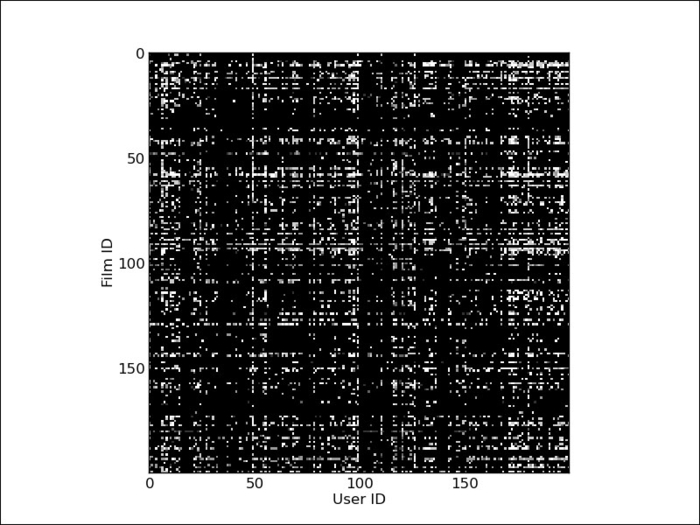
We can visualize the values of the matrix as an image where each rating is depicted as a little square. Black represents the absence of a rating and the grey levels represent the rating value. We can see that the matrix is sparse—most of the squares are black. We can also see that some users rate a lot more movies than others and that some movies are the target of many more ratings than others.

The code to visualize the data is very simple (you can adapt it to show a larger fraction of the matrix than is possible to show in this book), as follows:

from matplotlib import pyplot as plt
imagedata = reviews[:200, :200].todense()
plt.imshow(imagedata, interpolation='nearest')

The following screenshot is the output of this code:

We are now going to use this binary matrix to make predictions of movie ratings. The general algorithm will be (in pseudocode) as follows:

Implementing the code first, we are going to write a simple NumPy function. NumPy ships with np.corrcoeff, which computes correlations. This is a very generic function and computes n-dimensional correlations even when only a single, traditional correlation is needed. Therefore, to compute the correlation between two users, we need to call the following:

  corr_between_user1_and_user2 = np.corrcoef(user1, user2)[0,1]

In fact, we will be wishing to compute the correlation between a user and all the other users. This will be an operation we will use a few times, so we wrap it in a function named all_correlations:

import numpy as np
def all_correlations(bait, target):
    '''
    corrs = all_correlations(bait, target)

    corrs[i] is the correlation between bait and target[i]
    '''
    return np.array(
            [np.corrcoef(bait, c)[0,1]
                for c in target])

Now we can use this in several ways. A simple one is to select the nearest neighbors of each user. These are the users that most resemble it. We will use the measured correlation discussed earlier:

def estimate(user, rest):
  '''
   estimate movie ratings for 'user' based on the 'rest' of the universe.
  '''
  # binary version of user ratings
    bu = user > 0
  # binary version of rest ratings
    br = rest > 0
    ws = all_correlations(bu,br)
  # select 100 highest values
    selected = ws.argsort()[-100:]
  # estimate based on the mean:
    estimates = rest[selected].mean(0)
  # We need to correct estimates
  # based on the fact that some movies have more ratings than others:
    estimates /= (.1+br[selected].mean(0))

When compared to the estimate obtained over all the users in the dataset, this reduces the RMSE by 20 percent. As usual, when we look only at those users that have more predictions, we do better: there is a 25 percent error reduction if the user is in the top half of the rating activity.

In the previous section, we looked at the users that were most similar. We can also look at which movies are most similar. We will now build recommendations based on a nearest neighbor rule for movies: when predicting the rating of a movie M for a user U, the system will predict that U will rate M with the same points it gave to the movie most similar to M.

Therefore, we proceed with two steps: first, we compute a similarity matrix (a matrix that tells us which movies are most similar); second, we compute an estimate for each (user-movie) pair.

We use the NumPy zeros and ones functions to allocate arrays (initialized to zeros and ones respectively):

movie_likeness = np.zeros((nmovies,nmovies))
allms = np.ones(nmovies, bool)
cs = np.zeros(nmovies)

Now, we iterate over all the movies:

for i in range(nmovies):
    movie_likeness[i] = all_correlations(reviews[:,i], reviews.T)
    movie_likeness[i,i] = -1

We set the diagonal to -1; otherwise, the most similar movie to any movie is itself, which is true, but very unhelpful. This is the same trick we used in Chapter 2, Learning How to Classify with Real-world Examples, when we first introduced the nearest neighbor classification. Based on this matrix, we can easily write a function that estimates a rating:

def nn_movie(movie_likeness, reviews, uid, mid):
    likes = movie_likeness[mid].argsort()
  # reverse the sorting so that most alike are in
   # beginning
    likes = likes[::-1]
  # returns the rating for the most similar movie available
    for ell in likes:
        if reviews[u,ell] > 0:
            return reviews[u,ell]

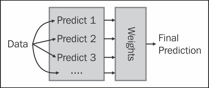
We can now combine the methods given in the earlier section into a single prediction. For example, we could average the predictions. This is normally good enough, but there is no reason to think that both predictions are similarly good and should thus have the exact same weight of 0.5. It might be that one is better.

We can try a weighted average, multiplying each prediction by a given weight before summing it all up. How do we find the best weights though? We learn them from the data of course!

Tip

Ensemble learning

We are using a general technique in machine learning called ensemble learning ; this is not only applicable in regression. We learn an ensemble (that is, a set) of predictors. Then, we combine them. What is interesting is that we can see each prediction as being a new feature, and we are now just combining features based on training data, which is what we have been doing all along. Note that we are doing so for regression here, but the same reasoning is applicable during classification: you learn how to create several classifiers and a master classifier, which takes the output of all of them and gives a final prediction. Different forms of ensemble learning differ on how you combine the base predictors. In our case, we reuse the training data that learned the predictors.

By having a flexible way to combine multiple methods, we can simply try any idea we wish by adding it into the mix of learners and letting the system give it a weight. We can also use the weights to discover which ideas are good: if they get a high weight, this means that it seems they are adding useful information. Ideas with very low weights can even be dropped for better performance.

The code for this is very simple, and is as follows:

  
  # We import the code we used in the previous examples:
  import similar_movie
  import corrneighbors
  import usermodel
  from sklearn.linear_model import LinearRegression

  es = [
    usermodel.estimate_all()
    corrneighbors.estimate_all(),
    similar_movie.estimate_all(),
  ]
  coefficients = []  
  # We are now going to run a leave-1-out cross-validation loop
  for u in xrange(reviews.shape[0]): # for all user ids
    es0 = np.delete(es,u,1) # all but user u
    r0 = np.delete(reviews, u, 0)
        P0,P1 = np.where(r0 > 0) # we only care about actual predictions
        X = es[:,P0,P1]
        y = r0[r0 > 0]
        reg.fit(X.T,y)
        coefficients.append(reg.coef_)
    prediction = reg.predict(es[:,u,reviews[u] > 0].T)
    # measure error as before

The result is an RMSE of almost exactly 1. We can also analyze the coefficients variable to find out how well our predictors fare:

  print coefficients.mean(0) # the mean value across all users

The values of the array are [ 0.25164062, 0.01258986, 0.60827019]. The estimate of the most similar movie has the highest weight (it was the best individual prediction, so it is not surprising), and we can drop the correlation-based method from the learning process as it has little influence on the final result.

What this setting does is it makes it easy to add a few extra ideas; for example, if the single most similar movie is a good predictor, how about we use the five most similar movies in the learning process as well? We can adapt the earlier code to generate the k-th most similar movie and then use the stacked learner to learn the weights:

es = [
    usermodel.estimate_all()
    similar_movie.estimate_all(k=1),
    similar_movie.estimate_all(k=2),
    similar_movie.estimate_all(k=3),
    similar_movie.estimate_all(k=4),
    similar_movie.estimate_all(k=5),
  ]
# the rest of the code remains as before!

We gained a lot of freedom in generating new machine learning systems. In this case, the final result is not better, but it was easy to test this new idea.

However, we do have to be careful to not overfit our dataset. In fact, if we randomly try too many things, some of them will work well on this dataset but will not generalize. Even though we are using cross-validation, we are not cross-validating our design decisions. In order to have a good estimate, and if data is plentiful, you should leave a portion of the data untouched until you have your final model that is about to go into production. Then, testing your model gives you an unbiased prediction of how well you should expect it to work in the real world.