Principal component analysis is often the first thing to try out if you want to cut down the number of features and do not know what feature extraction method to use. PCA is limited as it is a linear method, but chances are that it already goes far enough for your model to learn well enough. Add to that the strong mathematical properties it offers, the speed at which it finds the transformed feature space, and its ability to transform between the original and transformed features later, we can almost guarantee that it will also become one of your frequently used machine learning tools.

Summarizing it, given the original feature space, PCA finds a linear projection of it into a lower dimensional space that has the following properties:

As PCA simply transforms the input data, it can be applied both to classification and regression problems. In this section, we will use a classification task to discuss the method.

Applying PCA

Let us consider the following artificial dataset, which is visualized in the left plot as follows:

>>> x1 = np.arange(0, 10, .2)
>>> x2 = x1+np.random.normal(loc=0, scale=1, size=len(x1))
>>> X = np.c_[(x1, x2)]
>>> good = (x1>5) | (x2>5) # some arbitrary classes
>>> bad = ~good # to make the example look good

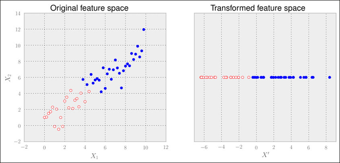
Scikit-learn provides the PCA class in its decomposition package. In this example, we can clearly see that one dimension should be enough to describe the data. We can specify that using the n_components parameter:

>>> from sklearn import linear_model, decomposition, datasets
>>> pca = decomposition.PCA(n_components=1)

Here we can also use PCA's fit() and transform() methods (or its fit_transform() combination) to analyze the data and project it into the transformed feature space:

>>> Xtrans = pca.fit_transform(X)

Xtrans contains only one dimension, as we have specified. You can see the result in the right graph. The outcome is even linearly separable in this case. We would not even need a complex classifier to distinguish between both classes.

To get an understanding of the reconstruction error, we can have a look at the variance of the data that we have retained in the transformation:

>>> print(pca.explained_variance_ratio_)
>>> [ 0.96393127]

This means that after going from two dimensions to one dimension, we are still left with 96 percent of the variance.

Of course, it is not always that simple. Often, we don't know what number of dimensions is advisable upfront. In that case, we leave the n_components parameter unspecified when initializing PCA to let it calculate the full transformation. After fitting the data, explained_variance_ratio_ contains an array of ratios in decreasing order. The first value is the ratio of the basis vector describing the direction of the highest variance, the second value is the ratio of the direction of the second highest variance, and so on. After plotting this array, we quickly get a feel of how many components we would need: the number of components immediately before the chart has its elbow is often a good guess.

Tip

Plots displaying the explained variance over the number of components is called a Scree plot. A nice example of combining a Scree plot with a grid search to find the best setting for the classification problem can be found at http://scikit-learn.sourceforge.net/stable/auto_examples/plot_digits_pipe.html.

Being a linear method, PCA has its limitations when we are faced with data that has non-linear relationships. We won't go into details here, but it will suffice to say that there are extensions of PCA, for example Kernel PCA, which introduce a non-linear transformation so that we can still use the PCA approach.

Another interesting weakness of PCA that we will cover here is when it is being applied to special classification problems.

Let us replace the following:

>>> good = (x1>5) | (x2>5)

with

>>> good = x1>x2

to simulate such a special case and we quickly see the problem.

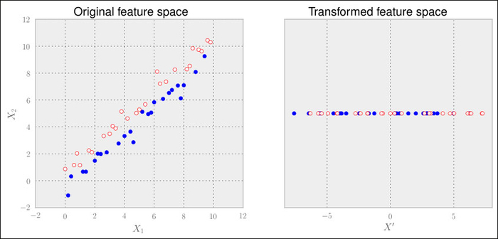
Here, the classes are not distributed according to the axis with the highest variance but the one with the second highest variance. Clearly, PCA falls flat on its face. As we don't provide PCA with any cues regarding the class labels, it cannot do any better.

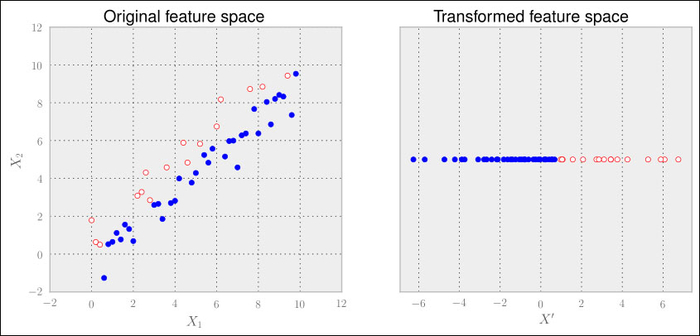
Linear Discriminant Analysis (LDA) comes to the rescue here. It is a method that tries to maximize the distance of points belonging to different classes while minimizing the distance of points of the same class. We won't give any more details regarding how the underlying theory works in particular, just a quick tutorial on how to use it:

>>> from sklearn import lda
>>> lda_inst = lda.LDA(n_components=1)
>>> Xtrans = lda_inst.fit_transform(X, good)

That's all. Note that in contrast to the previous PCA example, we provide the class labels to the fit_transform() method. Thus, whereas PCA is an unsupervised feature extraction method, LDA is a supervised one. The result looks as expected:

Then why to consider PCA in the first place and not use LDA only? Well, it is not that simple. With the increasing number of classes and less samples per class, LDA does not look that well any more. Also, PCA seems to be not as sensitive to different training sets as LDA. So when we have to advise which method to use, we can only suggest a clear "it depends".