
After applying performance testing on one web test at a time and after measuring the underlying system's metrics, Test Studio extends these possibilities by simulating multiples of this request and multiples of the user executing it. During such scenarios, a network of users will be created and managed so that they perform the anticipated activities. This is all achieved with Test Studio's ability to multithread sessions and to simulate a load on the tested server.
The following section starts by understanding various Test Studio load components architecture, communications, and responsibilities to prepare for the load plan illustrated and executed afterwards inside Test Studio.
This section describes Test Studio 2012 R2 Version architecture, and the way it works in order to achieve a correct simulation of real-life system usage in terms of users and application transactions. Nevertheless, Test Studio does not confine to this only since the simulation alone is certainly barely revealing anything. It is mostly about the underlying metric numbers. Hence it is critical to have access to the necessary KPIs and a calculated set of metrics in order to accurately interpret the results. Test Studio is internally equipped with adequate services, providing all the functionalities mentioned earlier, which we are going to see in detail.
Similar to other tests, Test Studio IDE is the workspace that presents the capabilities for constructing the load tests and designing their load strategy. It also serves as the portal that initiates test execution and communication with other remote Test Studio services. The Load Controller is the Test Studio load simulation manager. This component is responsible for closely managing the load execution and orchestrating all load agents. The Load Agent is the component that controls the virtual users that produce the load traffic. Depending on your load-testing plan, you might want to have more than one load agent distributed on different machines with different specifications to imitate a real-life environment. Finally, the Load Reporter is the component that records the load test. It connects to the Load Controller in order to retrieve statistics and save them in a SQL database. The last section of this chapter deals with external reports and will explain the tables of this database.
To be able to make use of the components mentioned earlier, they will have to be installed on the target machine first. The following link belongs to the Telerik online documentation for Test Studio and explains how to install Test Studio services: http://www.telerik.com/automated-testing-tools/support/documentation/user-guide/load-testing.aspx.
As with performance testing, in order to successfully run your tests, all Test Studio services must be running correctly. Launch Test Studio services configuration manager from the start menu by going to Start | All Programs | Telerik | Test Execution | Configure Load Test Services.
After the window opens, make sure all services are running and the Start button is disabled. For every service, you can optionally change the network interface and TCP/IP port number. Most likely, the different load components will not be present on the same machine. Therefore, you have the flexibility to change the hosting machine.
The configuration manager section for Load Controller is shown in the following screenshot:
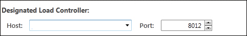
Configuring load controller
The following screenshot displays the section concerned with the Reporter service. This part of the window allows editing of the SQL database used by the Load Reporter. Note that in case the database name is changed, the newly provided database must contain all the tables used by the Reporter instance. This means that Test Studio will not create the missing database object, if any. Hence, in summary, there are two ways to guarantee a proper reporting database, either by letting Test Studio create one for you during installation or by downloading the relevant scripts from this link: http://www.telerik.com/automated-testing-tools/support/documentation/user-guide/load-testing/generating-reports-from-sql-database.aspx. Once the database is created, the final step is to pass the newly created database parameters to the configuration window, as shown in the following screenshot:
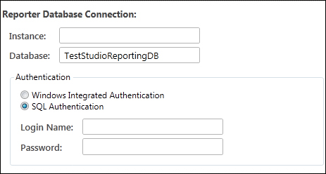
Configuring the reporting database
The last section of this window holds the properties for the logfile. This file is used by Test Studio to write down logs from the different load services. Optionally, logging can be enabled or disabled using the fields shown in following screenshot. This logfile can grow large rapidly, so it is preferable to enable the logging option only for troubleshooting purposes.
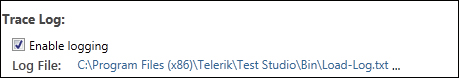
Configuring logging
In this section, we will see the structured load testing process, which begins by setting the expectations around the system usage in real life. Hence, before using Test Studio load capabilities, we are going to walk through a sample plan that was exercised on the BugNet application used in the previous chapter. After defining the KPIs that need to be monitored, the load characteristics for this plan will be implemented step by step.
As with any testing type, the load-testing process should be thoroughly planned in order to bring the testing work closer to the real usage of the application. This phase includes estimation of the different variables that parameterize load testing. The principle elements that are going to dominate our estimates for this section are the users and their types of activities.
Some goals were extracted based on the objectives and expectations drawn for the project when nonfunctional application performance was tackled. These goals help in assessing objectives and avoiding materialization of key concerns by keeping an open eye.
The first goal is related to response time, where no request is allowed to exceed 2.5 seconds for any type of transaction, since this will cause the user to abandon the operation. The second goal is related to HTTP errors, where we allow at most five errors per second. The third goal tackles the issue of efficiency in handling transactions by the server—we seek to achieve at least 50 transactions per second.
So how will the preceding goals behave when the system is exposed to certain loads?
These loads consist of numerous combinations of transactions coming from different user types. Hence, the purpose of the next section is to narrow down these combinations by designing user workloads.
Designing workloads starts firstly by estimating the projected number of users that are going to use BugNet.
Secondly, it proceeds by approximating the share that each transaction partakes of the overall usage of the system. Knowing also that transactions are categorized with the types of users (enumerated in the previous chapters), the estimated shares must also take into consideration the percentage of each user type of the overall number concluded in the previous step.
The estimates derived from the BugNet application are contained in the answers to the following series of questions:
- What is the projected number of users?
We are considering each project hosted on BugNet will have 100 members divided into membership groups, as appearing in the following table. On an average, we expect to have 10 projects for a deployed BugNet version.
The member distribution inside a group is as follows:
User types
Estimated numbers
Project Administrator
1
Quality Assurance
44
Developers
44
Reporters
11
- What is the percentage of concurrent users?
The estimated percentage of concurrent users are as follows:
User types
Estimated percentages
Project Administrator
5%
Quality Assurance
50%
Developers
35%
Reporters
10%
- What is the length of user sessions?
The estimates length of user sessions are as follows:
User types
Estimated session length (min)
Project Administrator
30
Quality Assurance
300
Developers
120
Reporters
60
- What is the percentage of each activity for each user type?
The estimated percentage of each activity for each user type is as shown in the following tables:
- Project Administrator:
Activity types
Estimated percentages
Logging in
20%
Configuring BugNet settings
10%
Creating and editing projects
50%
Creating user accounts
20%
- Quality Assurance Engineers:
Activity types
Estimated percentages
Logging in
20%
Posting incidents
30%
Updating incident details and commenting on an incident
45%
Performing queries
5%
- Developers:
Activity types
Estimated percentages
Logging in
20%
Commenting on incidents
70%
Performing queries
10%
- Reporters:
Activity types
Estimated percentages
Logging in
20%
Performing queries
80%
- Project Administrator:
After performing the calculations, the following total percentages are extracted for each activity:
|
Activity types |
Estimated percentages |
|---|---|
|
Logging in |
20% |
|
Configuring BugNet settings |
0.5% |
|
Creating and editing projects |
2.5% |
|
Creating user accounts |
1% |
|
Posting incidents |
15% |
|
Updating and commenting on incidents |
47.5% |
|
Performing queries |
13.5% |
The preceding estimation serves in deducing the baseline tests. In fact, the left column of the last table corresponds to the list of tests to be used further on in load testing. The operations of logging in, creating user accounts, posting incidents, and performing queries were already automated in the pervious chapter, and they map to Perf_Login, Perf-1_NewAccount, Perf-2_NewIssue, and Perf-3_PerformQuery respectively. In addition to these tests, the following sections are going to make use of other powerful capabilities available inside Test Studio in order to automate the remaining tests, such as updating and commenting BugNet incidents.
During implementation, we take the base tests and make sure they are present in an automated version inside Test Studio. Afterwards, we plug in all the estimated numbers in the test designs. For this purpose, we are going to discover next a new template made available by Test Studio in order to perform load testing.
Start first by creating the folder that is going to hold all the subsequent tests. Rename it as Load Tests. Under this folder, add a new test based on the Load Test template depicted in the following screenshot and call it Load-1:
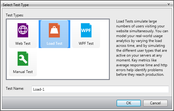
Creating a load test
Double-click on the added test to enter its edit mode. The first step starts by configuring the environment in which the test is going to run. This means we are going to specify the different Test Studio services that will handle and manage test execution. Subsequent to this, we reach the actual creation of the test requests and the specification of the planned load.
From the Steps ribbon, click on the Environment button appearing in the following screenshot:
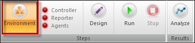
The Environment configuration button
This button opens the workspace that is shown in the following screenshot:
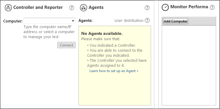
Load test workspace
We start from the first pane to the left, which is responsible for configuring the Controller and Reporter machines.
As mentioned earlier, the Controller will manage the test execution whereas the Reporter will handle the test results and their storage inside the database. The following screenshot shows the section related to specifying the machine hosting these services, where the connection to it was successful:
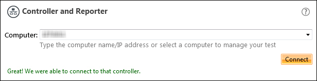
Configuring the machine hosting controller and reporter services
It is in the Computer field that the specification of the machine name or IP is entered. After filling it, the connection must be validated, so click on the Connect button. If the connection was successful, the label in green will be displayed as shown in the preceding screenshot. The connection has to be successful for us to proceed. Some reasons why the connection cannot be established are:
- Misspelling the machine name or IP
- The services are not started
- The services and Test Studio release versions are different
- Network settings problem
The Agents pane, which corresponds to the middle pane, displays the detected agents. During the execution of the load test, the Controller will evenly distribute the virtual users across the available Load Agents. The following screenshot is a sample of how Test Studio lists the test agents inside this section:
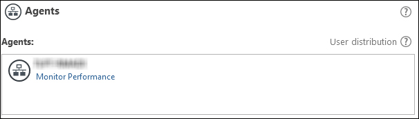
Load agents
As a result of our work, the ribbon has an indicator to relay to us whether all connections were successful. The green circles shown in the following screenshot signify that the services are reachable; on the other hand, a red circle suggests a failing configuration, which requires further investigation.
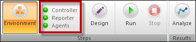
A successful connection to load services
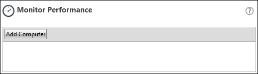
The last pane, the Monitor Performance pane, enables us to add the list of computers to be monitored. The Measurements section of this chapter has introduced some metrics calculated implicitly by Test Studio. Thus, after deriving the performance deficiency points, KPIs are then used for troubleshooting the results and identifying the root causes. So, as we did with performance testing, we are going to select the performance counters to be monitored throughout the test execution. The following screenshot shows the performance monitoring workspace:
Configuring computers for performance monitoring
Click on the Add Computer button appearing in the screenshot. Following this, the Monitor Performance window shown in the following screenshot is invoked:
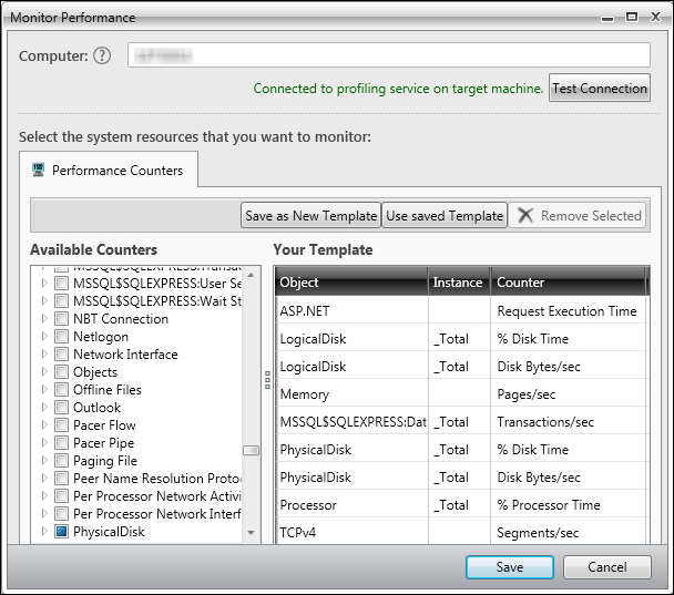
Choosing performance counters
To configure the computer, enter the name or IP of the machine to be monitored in the Computer field and then click on the Test Connection button to confirm that the target machine is reachable.
The next step is to add the counters that need to be monitored. The Performance Counters section shows a list that correspond to the Windows Performance Monitor counters that are native to Windows systems. We will select the same list of performance counters used in the previous chapter, which was saved in a template. So, browse for the BugNet template after clicking on the Use Saved Template button.
Click on the Save button and notice how an entry is added under the list of monitored computers.
With this, we have wrapped up the environment configuration.
The design stage comes after the test environment setup. We have arrived at the Design button of the Steps ribbon, shown in the following screenshot:
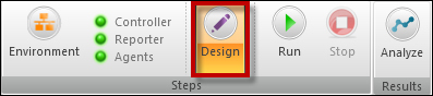
The Design button
This stage comprises of two main steps: defining user profiles and specifying the corresponding test settings. The left pane, titled Define User Profiles and Workload and shown in the following screenshot, will receive the user activities planned in the first phase. These activities will be saved in the form of HTTP requests and can be created or supplemented using four different ways, as we will see. Following the completion of these activities, we specify the Test Studio workload, which maps to the estimated percentage of users out of the overall targeted number of virtual users.
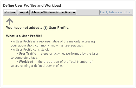
Profile and workload panel
To record a new test or to import an already created web test, click on the Capture button.

Capturing a new scenario
The Capture window is invoked and displays two options. Hence, to capture traffic for a new test, the Capture New button should be clicked. This will launch a new browser instance of our choosing and record the traffic for the requests initiated during the session. Alternatively, click on the Capture from existing Web Test button to import an existing test created using the web template.
On clicking on the Capture from existing Web Test button, the Select a test to capture section is enabled as shown in the preceding screenshot. This section will list the web tests created in the previous chapter. Select Perf-3_PerformQuery.
Knowing that browser types can also influence the performance of requests, this window offers a choice between multiple supported browsers. So choose the Internet Explorer icon from the Choose browser section.
Once a browser type is chosen, Test Studio will automatically execute the test steps in order to record the underlying HTTP traffic. An Edit User Profile window is invoked on the execution termination and has the Dynamic Targets window open directly on top of it. The latter window contains variables used by BugNet to generate information for the replayed requests. The dynamic targets are variables with assigned values sent from the server to the client. Subsequently, they will be used by the client, where it will generate further requests by passing these values as parameters. Test Studio automatically detects dynamic targets and displays them in a list as shown in the following window:
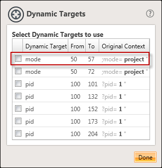
Selecting dynamic targets
In order to observe more closely how these variables work, we will take the example of the row highlighted in red.
The Dynamic Target column holds the name of the variable. The From column holds the request ID where the dynamic variable will be located in its response. The To column holds the request ID where the dynamic variable is used as a parameter. Finally, the Original Context column displays how this variable appears in the response. Before we see these column values inside the list of requests, we need to close the Dynamic Targets window. However, prior to this and in order to correctly replay the requests from the virtual users, we need to make sure these parameters are resent to the server; so select all variables displayed in the window and click on the Done button. While automating your tests, the best way to decide whether or not to include a target is to ask the developers. They will provide correct answers on the criticality of adding these variables as dynamic targets.
At this point, we have the Edit User Profile window enabled. The Name field carries the test name. The User Traffic panel to the left has the list of all the requests that were recorded during execution. The following screenshot shows a snippet of the requests list, where the 50th request is highlighted:
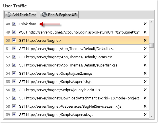
Load test user traffic
The Dynamic Targets window says that we should be able to find the value under the Original Context column in the response of the 50th request. The following screenshot shows the response, which is reachable by selecting the request and clicking on the Response tab inside the right-hand side pane that displays the details:

The Response tab having the dynamic target
The Response section contains outlined text that confirms the sought value. This value is passed as a parameter in request number 57, which is shown in the preceding screenshot.
The Edit User Profile window also offers another capability. Usually, when using an application in real time, there are certain delays on the client side that are not comprised in any time latency spent over the different application components. These delays correspond to the time taken by the user to think, which normally occur between UI operations performed against the screen. This inactivity at the client side represents the time taken by the user to analyze and prepare for the second action. Fortunately, Test Studio has a notion for this type of time and materializes it with think time steps. The previous screenshot for User Traffic contains this step and it is at position 48.
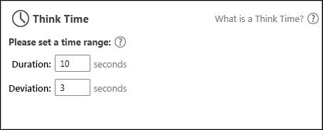
By default, Test Studio will insert the think time steps between the test steps. The think time details can be adjusted after selecting it. Again, the right-hand side pane will display the details as shown in the following screenshot. The Duration property stands for the idle time whereas Deviation is the factor of randomization added to the former property. This means that for the same Think Time step, the idle time can be any value between 7 and 13 seconds.
Setting the think time range
Click on the Save button to finish the creation of the user traffic that corresponds to performing a query web test. Repeat the same steps to import the following tests.
Perf-LoginPerf-1_NewAccountPerf-2_NewIssue
The second alternative for adding user profiles is through importing an already existing web test or previously recorded fiddler traffic in the SAZ files. This can all be performed through the Import button of the Define User Profiles and Workload panel. The following window opens after clicking on the Import button:
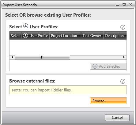
Importing external user scenarios
Click on the Browse button and attach the file called Updating and Commenting incidents.saz, which is produced from the fiddler after carrying out a test to edit the comment for an already posted bug on BugNet.
To sum up, we have now created five different activities for various BugNet users. The user profiles are not completed before we specify the corresponding workloads. Under the Workload column, adjust the slider for each test to comply with the following screenshot. The values were extracted from the User types table generated during the planning phase.
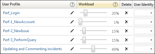
Specifying workloads for user profiles
The preceding screenshot also shows a User Identity column. When the scenario to be automated requires Windows authentication, you can create identities using the Manage Windows Authentication button and then assign them from the combobox. When the test executes, it will impersonate the user with the assigned Windows identity.
The final stage of the implementation phase is to set up the behavior of virtual user creation.
In some cases of load testing, you might want to test a full-blown scenario, where all users log in concurrently and start carrying out their tasks. Such cases appear in spike tests, which was explained near the chapter start. These situations could occur, for example, after restarting the web server in the middle of working hours. Once the application becomes available again, all the users that had open sessions will rush to log in in order to resume their work. However, this is not always the case. Normally, we will detect the sessions being incremented bit by bit until reaching a saturated number. In fact, this is useful to observe the application's nonfunctional behavior in handling a growing number of requests throughout its usage. We are going to see next how to make this happen inside Test Studio.
- The following screenshot shows the right-hand side panel of the Design work area:
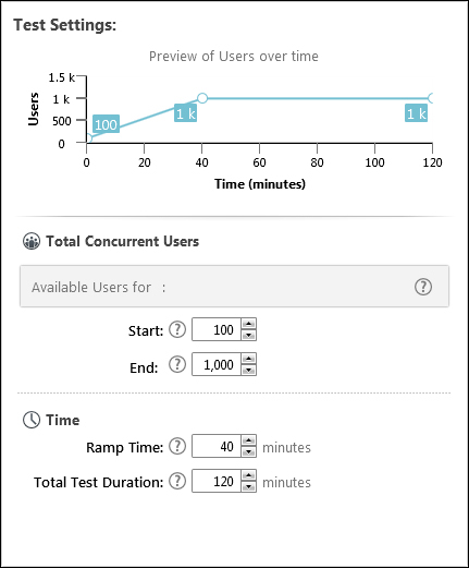
The first section of this panel is a dynamic chart line that automatically updates following the modification of the numbers appearing in the sections underneath. The Total Concurrent Users section has two variables. The Start field holds the number of parallel users that will start executing the user profiles as soon as the test is ready to start sending requests. The End field holds the maximum number of users that will be reached and maintained throughout the remaining time of the test. The period of time during which the number of users increases from start to end is ambiguous until now. It is specified in the Time section by setting the value for the Ramp Time field. This value represents the initial duration through which the creation of virtual users will grow from 100 to hit 1000 users. These numbers are extracted from the Designing workload section of this chapter, where they correspond to the number of estimated project members and the number of estimated project members multiplied by that of the estimated number of projects respectively. In our case, we need 40 minutes for the number of virtual users to be saturated, which is the estimated time required for employees (represented by virtual users) to log in to the BugNet in real life. Finally, the test will run for 120 minutes (two continuous hours of various BugNet activities), where each activity type will execute according to the designated percentages.
During this phase, additional test settings are specified at the level of the executing instance before we actually run the test. We will start by instructing Test Studio how frequently we wish to have our performance counters sampled. Afterwards, we proceed to the goals assignment.
This section is the last step in load test creation and execution. We are going to discover the last button in the Steps ribbon, shown in the following screenshot:
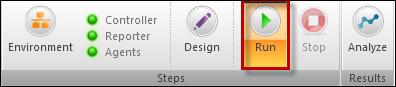
The Run button for load tests
Click on the Run button to enable and edit the run settings.
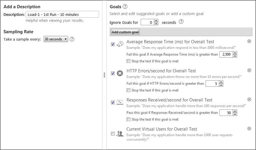
Execution settings for load tests
The left-hand side panel contains the Description property, which is a free input field allowing the user to enter information about the specific execution instance in text. The Sampling Rate dropdown allows the selection of the intervals at which the sampling is going to take place. In this example, the test will run for 10 continuous minutes, where performance data will be recorded every 30 seconds and saved for later analysis.
The right-hand side panel is responsible for specifying the goals, where four are originally displayed by Test Studio in an inactive state. They will not have any effect on the execution unless we check their corresponding checkboxes. Therefore, the preceding screenshot shows some entries that have been enabled to reflect the goals defined in the Defining goals section of this chapter. Based on these numbers, Test Studio will, by default, only alert the user and color the metrics that do not satisfy these thresholds in red. Optionally, we can choose to abort the test execution if any of the underlying rules is violated. This depends on how critical the goal is.
Other metric rules can be added on top of the default goals list by clicking on the Add custom goal button. The ensuing window will allow you to build your own verification expression and again choose whether there is a need to interrupt test execution in case it is not satisfied. The following screenshot shows the pool of goal operands that can be chosen:
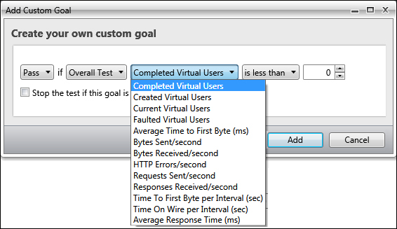
Adding custom goals
Click on the Run this test button and wait until the execution finishes.
We have now entered the analysis phase. The data gathered during execution will be available to use after clicking the Analyze button of the Results ribbon.
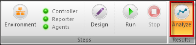
The Analyze result button for load tests
A built-in automatic reporting mechanism is available inside Test Studio under three contexts. The DASHBOARD view has a summary of the metrics seen in the Measurements section of this chapter. The following screenshot shows an example of a run result for this load test:
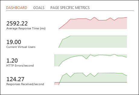
The Dashboard view of test results
Notice how the average response time is colored in red since it has surpassed the designated threshold. The curves corresponding to the other metrics are colored in green, which means that they lie in the targeted goal range.
The GOALS tab shown in the preceding screenshot holds a more detailed view of the assigned goals. It compares the actual numbers against the targeted ones for every goal. Finally, the PAGE SPECIFIC METRICS tab offers very important information at a page level. The total errors and the average response times are calculated for each URL and displayed in a grid view.
Other test result tabs are also available in case we want to further examine the relation between the average response time and the virtual users, investigate why there has been a steep rise in HTTP errors, or troubleshoot the sudden fall in responses received over the entire test execution duration. Additionally, we may want to see how the performance counters that were assigned in the test design stage are acting. We may also want these metrics to contribute to some complex charts. And finally, as executions are being re-run after performance adjustments, we would like to compare the resulting curves from each run on one graph. In these cases, we are looking for more advanced charts and Test Studio offers these capabilities through its custom charts.
While on the Analyze tab, the left-hand side pane has the list of test executions. Each execution entry holds the date and time of execution and two other buttons, as depicted in the following screenshot:
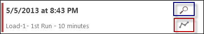
A test execution entry in the Analyze tab
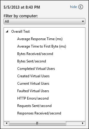
The magnifier (the top button in the preceding screenshot) contains the dashboard, goals, and page metrics for a single run, which have been described earlier. The chart line (also highlighted in the preceding screenshot) gives the ability to construct user-defined charts. Click on this button; a collapsible panel appears. It contains the list of metrics automatically measured with Test Studio in addition to the counters that were manually initially selected for monitoring purposes. For a more focused analysis, they can be filtered by any of the set of monitored machines through the Filter by computer combobox.
The performance metrics chart panel
The first chart that we are going to build draws the correlation between the response time and concurrent virtual users. Select Average Response Time, Current Virtual Users, and Created Virtual Users from the metrics panel to enable them. The resulting chart is shown in the following screenshot:
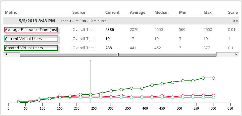
The response time with respect to virtual users
The horizontal axis corresponds to the time measured in seconds. It starts at 0 and ends at 600 seconds, which corresponds with the 10 minutes specified for the overall test execution duration. On this graph, we have three plotted curves. Each stands for a certain metric and is recognizable by its color.
At first, notice how it takes 2 minutes for the gradually increasing number of current users to reach its maximum—starting at second 30 and ending at second 150. The lowermost blue curve corresponds to the current virtual users, and it stabilizes after reaching the maximum number of intended users during the load test. This means that at any point greater than 150, the number of concurrent active users involved in application transactions corresponds to the maximum value. The purpose of this ramp-up behavior is to simulate the real-life usage of the system and study its capacity to process transactions from an incremental load injected users.
During the overall test execution, the created virtual users will deprecate after accomplishing their designated BugNet operations. Meanwhile, Test Studio will counter this user declination with the creation of additional ones to maintain the overall number of concurrent users throughout the test duration. This is where the created virtual users' line on the chart comes into the picture. This is the uppermost line colored in green and as expected it should be strictly incrementing from start to end to make up for the destroyed virtual users. Another hidden implication also lies behind the total created virtual users' line, where the greater the number of created users is, the faster the application will process transactions. This is because Test Studio will have to create more users to compensate for the destroyed ones.
Finally, the response time middle line in red represents the time spent on the client side while awaiting the receipt of the last byte of the response. Sudden spikes in the line could hint at overloaded situations, which require further investigation in order to isolate the component that is causing the bottleneck. Response time charts also help in finding the tipping point, over which the system will no longer be able to process requests. Moreover, the trend of these lines is useful in expressing the scalability, where the system is assumed to be more scalable if the line increases in a flat manner. Steps in the response time lines can signify dangerous behaviors since the number of users and response times are not regularly proportional.
We are going to dwell just a bit more on this chart to examine some statistics already calculated by Test Studio. Notice that the table has many headers related to some key statistical information: Average, Median, Min, and Max. They are intuitive metrics and provide useful information, as designated by their titles. For example, the response time average is 2079 milliseconds; its lowest value was 569 and its peak point reached 2650 milliseconds. The median is equal to 2650 milliseconds and it occurs at second 330. This point is found on the horizontal axis after summing the regular middle point to the warm up time at the beginning. The warm up time displays neither user creation nor request execution. Another handy column is Current. As we slide the vertical slice line over the horizontal axis, this column will be dynamically populated with changing values corresponding to the intersection of each curve with the bar. In the preceding chart, at approximately 240 seconds, the current virtual users had already reached its peak, the created virtual users that far was 288, and the response time for the executing request was 2386 milliseconds.
The second chart we are going to build represents the amount of responses received per second. To clear any line already present on the chart, either click on the corresponding metric again to deselect it or click on the x button at the end of the row in the chart table to remove it. Clear Created Virtual Users and Average Response Time and replace them with Response Received/second. The following chart shows the resultant graph after updating the metrics:
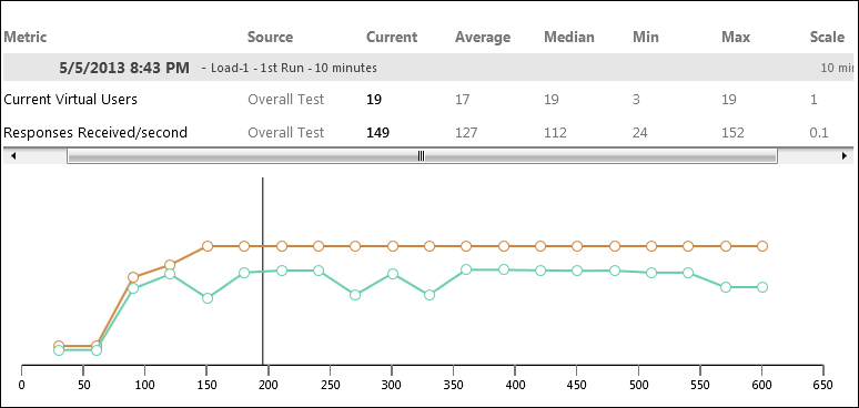
Responses per second with respect to the current virtual users
So far we have restricted our charts to results captured during one execution. Test Studio's great advantage in reporting is that it enables the ability to easily compare multiple runs against each other. This is why it will always keep the execution results for future reference.
So as the improvements are applied to the components causing bottlenecks, it is time to plot the repetitively captured KPIs generated from this component on one chart. For this purpose, we will use Test Studio custom charts once again.
Firstly, make a new run of the same test. The Analyze your results pane in the Analyze view now holds two entries sorted by ascending order based on the date value. Enable the metrics panel for any of the execution runs. Locate the node that represents the machine that was chosen for performance monitoring and select the metric corresponding to the total processor time. Repeat the same steps for the other run. This will cause both curves to be plotted on the same chart, as shown in the following screenshot:
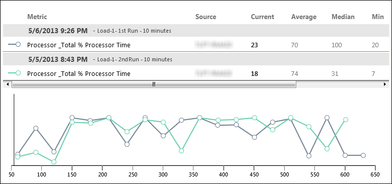
Comparing two executions
The upper section has the table displaying the lists of the runs that participate in the chart whereas the lower section contains the two lines corresponding to the processor time behavior in each run.
The customization and analysis of the load results is not limited in Test Studio since in addition to the user-defined charts that we have just seen, Test Studio extends its reporting power to SQL server too.
During the services configuration stage, a section was available to set up the SQL database that is going to be used by the reporting service in order to record the data indicators that are being captured. The following screenshot describes the reporting database:
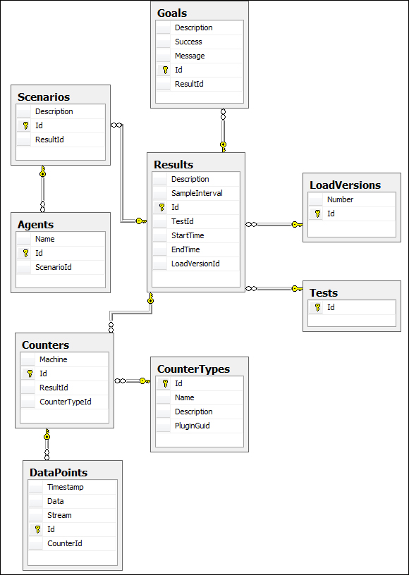
The reporting database diagram
The following list explains the usefulness of each type of data present inside the various tables:
- Tests: This table contains the list of tests created using the load template and are uniquely identified by their GUID
- LoadVersions: This table contains the Test Studio load versions managing load testing
- Results: This table contains the results for each execution instance (recognized by its
Descriptionfield, which maps theDescriptioncolumn in the table) and they mainly map to theTestsandLoadVersionsprimary keys - Goals: This table has the goals (recognized by their
Messagecolumn) that were assigned for each test at the design stage, and since they can vary per execution instance, they mainly link to the Results table primary key - Scenarios: This table contains the load testing scenarios
- Agents: This table has the list of Test-Studio-installed load agents
- CounterTypes: This table has the predefined list of performance counters (recognized by the
Namecolumn) that can be monitored during load execution and which were available while preparing the environment of a load test - Counters: This table has the list of counters that were effectively selected for performance monitoring throughout executions for all tests; since they can differ for every execution instance, they depend on the
Resultstable primary key - DataPoints: This table contains the actual values gathered for the counters in each executing test instance, so they depend on the
Countersprimary key
This pool of rich test results along with their distribution among the SQL tables provides the power to perform any suitable comparison in the context of our analysis. For example, the following chart represents the percentage of goals that has been met out of the original number of assigned goals. This percentage is applied for all the execution instances of a specific test.
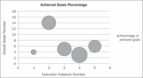
The percentage of achieved goals chart
Three types of variables are used to draw this chart. The horizontal axis represents a number increasing from one to six. It represents the number assigned for each load test execution instance. The vertical axis has the number of goals that was set for each of these instances. The Percentage of achieved goals calculates the number of goals that passed with respect to the overall number. They are represented on the charts by the blue bubbles. The size of the bubble helps to visually capture performance discrepancies between the multiple executing instances of the test.
Finally, the T-SQL(Transact-SQL) query that was used to retrieve the underlying chart table is as follows:
SELECT Results.Description,
COUNT(Goals.Description) AS NumGoals,
SUM(CONVERT(Decimal, Goals.Success))/COUNT(Goals.Description)*100 AS percentagePassed
FROM [TestStudioReportingDB].[dbo].[Results] INNER JOIN Tests ON Results.TestId = Tests.Id
INNER JOIN Goals ON Results.Id = Goals.ResultId
WHERE Tests.Id = '149C299B-E5D6-45B1-9F82-2FDA040D144E'
GROUP BY Results.Description