4.4. The Finite Field Discrete Logarithm Problem

The discrete logarithm problem (DLP) has attracted somewhat less attention of the research community than the IFP has done. Nonetheless, many algorithms exist to solve the DLP, most of which are direct adaptations of algorithms for solving the IFP. We start with the older algorithms collectively known as the square root methods, since the worst-case running time of each of these is for the field . The new family of algorithms based on the index calculus method provides subexponential solutions to the DLP and is described next. For the sake of simplicity, we assume in this section that we want to compute the discrete logarithm ind_g a of with respect to a primitive element g of . We concentrate only on the fields , p odd prime, and , , since non-prime fields of odd characteristics are only rarely used in cryptography.

4.4.1. Square Root Methods

Square root methods are applicable to any finite (cyclic) group. To avoid repetitions we provide here a generic description. That is, we assume that G is a multiplicatively written group of order n and . The identity of G is denoted as 1. It is not necessary to assume that G is cyclic or that g is a generator of G. However, these assumptions are expected to make the descriptions of the algorithms somewhat easier and hence we will stick to them. The necessary modifications for non-cyclic groups G or non-primitive elements g are rather easy and the reader is requested to fill out the details. We assume that each element of G can be represented by O(lg n) bits (so that the input size is taken to be lg n) and that multiplications, exponentiations and inverses in G can be computed in time polynomially bounded by this input size.

Shanks’ baby-step–giant-step method

Let us assume that the elements of G can be (totally) ordered in such a way that comparing two elements of G with respect to this order can be done in polynomial time of the input size. For example, a natural order on is the relation ≤ on . Note that k elements of G can be sorted (under the above order) using O(k log k) comparisons.

Let . Then d := ind_g a is uniquely determined by two (nonnegative) integers d₀, d₁ < m such that d = d₀ + d₁m (the base m representation of d). In Shanks’ baby-step–giant-step (BSGS) method, we compute d₀ and d₁ as follows. To start with we compute a list of pairs (d₀, g^d₀) for d₀ = 0, 1, . . . , m – 1 and store these pairs in a table sorted with respect to the second coordinate (the baby steps). Now, for each d₁ = 0, 1, . . . , m – 1, we compute g^–md₁ (the giant steps) and search if ag^–md₁ is the second coordinate of a pair (d₀, g^d₀) of some entry in the table mentioned above. If so, we have found the desired d₀ and d₁, otherwise we try with the next value of d₁. An optimized implementation of this strategy is given as Algorithm 4.6.

The computation of all the elements of T and sorting T can be done in time O^~(m). If we use a binary search algorithm (Exercise 4.15), then the search for h in T can be performed using O(lg m) comparisons in G. Therefore, the giant steps also take a total running time of O^~(m). Since , the BSGS method runs in time . The memory requirement of the BSGS (that is, of the table T) is . Thus this method becomes impractical, even when n contains as few as 30 decimal digits.

Pollard’s rho method

Pollard’s rho method for solving the DLP is similar in idea to the method with the same name for solving the IFP. Let be a random map and let us generate a sequence of tuples , , starting with a random (r₁, s₁) and subsequently computing (r_i+1, s_i+1) = f(r_i, s_i) for each i = 1, 2, . . . . The elements for i = 1, 2, . . . can then be thought of as randomly chosen ones from G. By the birthday paradox (Exercise 2.172), we expect to get a match b_i = b_j for some i ≠ j, after of the elements b₁, b₂, . . . are generated. But then we have a^r_i–r_j = g^{s_j –s_i}, that is, ind_g a ≡ (r_i – r_j)^–1(s_j – s_i) (mod n), provided that the inverse exists, that is, gcd(r_i – r_j, n) = 1. The expected running time of this algorithm is , the same as that of the BSGS method, but the storage requirement drops to only O(1) elements of G.

Algorithm 4.6. Shanks’ baby-step–giant-step method

Input: G, g and a as described above. Output: d = indg a. Steps: n : = ord(G), . /* Baby steps */ Initialize T to an empty table. Insert the pairs (0, 1) and (1, g) in T. h := g. for d0 = 2, . . . , m – 1 {     h := hg.     Insert (d0, h) in T. } sort T with respect to the second coordinate. /* Giant steps */ h := a. l := (g–1)m. for d1 = 0, . . . , m – 1 {     if T contains an entry (d0, h) { Return d := d0 + d1m. }     h := hl. }

The Pohlig–Hellman method

The Pohlig–Hellman (PH) method assumes that the prime factorization of n = ord is known. Since d := ind_g a is unique modulo n, we can easily compute d using the CRT from a knowledge of d modulo , j = 1, . . . , r. So assume that p is a prime dividing n and that . Let d₀ + d₁p + ··· + d_α–1p^α–1, , be the p-ary representation of d modulo p^α. The p-ary digits d₀, d₁, . . . , d_α–1 can be successively computed as follows.

Let H be the subgroup of G generated by h := g^n/p. We have ord H = p (Exercise 2.44). For the computation of d_i, , from the knowledge of d₀, . . . , d_i–1, consider the element

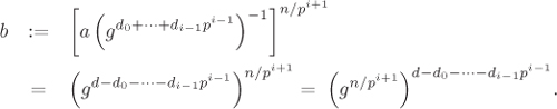
But ord(g^n/pi+1) = pⁱ⁺¹, so that

Thus, and d_i = ind_h b, that is, each d_i can be obtained by computing a discrete logarithm in the group H of order p (using the BSGS method or the rho method).

From the prime factorization of n, we see that the computations of d modulo for all j = 1, . . . , r can be done in time , q being the largest prime factor of n, since α_j and r are O(log n). Combining the values of d modulo by the CRT can be done in polynomial time (in log n). In the worst case, q = O(n) and the PH method takes time which is fully exponential in the input size log n. But if q (or, equivalently, all the prime divisors p₁, . . . , p_r of n) are small, then the PH method runs quite efficiently. In particular, if q = O((log p)^c) for some (small) constant c, then the PH method computes discrete logarithms in G in polynomial time. This fact has an important bearing on the selection of a group G for cryptographic applications, namely, n = ord G is required to have a suitably large prime divisor, so that the PH method cannot compute discrete logarithms in G in feasible time.

4.4.2. The Index Calculus Method

The index calculus method (ICM) is not applicable to all (cyclic) groups. But whenever it applies, it usually leads to the fastest algorithms to solve the DLP. Several variants of the ICM are used for prime finite fields and also for finite fields of characteristic 2. On such a field they achieve subexponential running times of the order of L(q, 1/2, c) = L[c] or L(q, 1/3, c) for positive constants c. We start with a generic description of the ICM. We assume that g is a primitive element of and want to compute d := ind_g a for some .

To start with we fix a suitable subset B = {b₁, . . . , b_t} of of small cardinality, so that a reasonably large fraction of the elements of can be expressed easily as products of elements of B. We call B a factor base. In the ICM, we search for relations of the form

Equation 4.5

for integers α, β, γ_i and δ_i. This gives us a linear congruence

Equation 4.6

The ICM proceeds in two^[4] stages. In the first stage, we compute d_i := ind_g b_i for each element b_i in the factor base B. For that, we collect Relation (4.5) with β = 0. When sufficiently many relations are available, the corresponding system of linear Congruences (4.6) is solved mod q – 1 for the unknowns d_i. In the second stage, a single relation with gcd(β, q – 1) = 1 is found. Substituting the values of d_i available from the first stage yields ind_g a.

^[4] Some authors prefer to say that the number of stages in the ICM in actually three, because they decouple the congruence-solving phase from the first stage. This is indeed justified, since implementations by several researchers reveal that for large fields this linear algebra part often demands running time comparable to that needed by the relation collection part. Our philosophy is to call the entire precomputation work the first stage. Now, although it hardly matters, it is up to the reader which camp she wants to join.

Note that as long as q (and g) are fixed, we don’t have to carry out the first stage every time the discrete logarithm of an element of is to be computed. If the values d_i, i = 1, . . . , t, are stored, then only the second stage needs to be carried out for computing the indices of any number of elements of . This is the reason why the first stage of the ICM is often called the precomputation stage.

In order to make the algorithm more concrete, we have to specify:

In the rest of this section, we describe variants of the ICM based on their strategies for selecting the factor base and for collecting relations. We discuss the third issue in Section 4.7.

4.4.3. Algorithms for Prime Fields

Let be a finite field of prime cardinality. For cryptographic applications, p should be quite large, say, of length around thousand bits or more, and so naturally p is odd. Elements of are canonically represented as integers between (and including) 0 and p–1. The equality x = y in means equality of two integers in the range 0, . . . , p–1, whereas x ≡ y (mod p) means that the two integers x and y may be different, but their equivalence classes in are the same.

The basic ICM

In the basic version of the ICM, we choose the factor base B to comprise the first t primes q₁, . . . , q_t, where t = L[ζ]. (The optimal value of ζ is determined below.) In the first stage, we choose random values of and compute g^α. Any integer representing g^α can be considered, but we think of as an integer in {1, . . . , p – 1}. We then try to factorize g^α using trial divisions by elements of the factor base B. If g^α is found to be B-smooth, then we get a desired relation for the first stage, namely,

If g^α is not B-smooth, we try another random α and proceed as above. After sufficiently many relations are available, we solve the resulting system of linear congruences modulo p – 1. This gives us d_i := ind_g q_i for i = 1, . . . , t.

In the second stage, we again choose random integers α and try to factorize ag^α completely over B. Once the factorization gets successful, that is, we have , we compute .

In order to optimize the running time, we note that the relation collection phase of the first stage is usually the bottleneck of the algorithm. If ζ (or equivalently t) is chosen to be too small, then finding B-smooth integers would be very difficult. On the other hand, if ζ is too large, then we have to collect too many relations to have a solvable linear system of congruences. More explicitly, since the integers g^α can be regarded as random integers of the order of p, the probability that g^α is B-smooth is (Corollary 4.1). Thus we expect to get each relation after random values of α are tried. Since for each α we need to carry out L[ζ] divisions by elements of the factor base B (the exponentiation g^α can be done in polynomial time and hence can be neglected for this analysis), each relation can be found in expected time . Now, in order to solve for d_i, i = 1, . . . , t, we must have (slightly more than) t = L[ζ] relations. Thus, the relation collection phase takes a total time of . It can be easily checked that is minimized for ζ = 1/2. This gives a running time of L[2] for the relation collection phase.

Since each g^α is a positive integer less than p, it is evident that it can have at most O(log p) prime divisors. In other words, the congruences collected are necessarily sparse. As we will see later, such a system can be solved in time O^~(t²), that is, in time L[1] for ζ = 1/2.

In the second stage, it is sufficient to have a single relation to compute d = ind_g a. As explained before, such a relation can be found in expected time . Thus the total running time of the basic ICM is L[2].

The second stage of the basic ICM is much faster than the first stage. In fact, this is a typical phenomenon associated with most variants of the ICM. Speeding up the first stage is, therefore, our primary concern.

Each step in the search for relations consists of an exponentiation (g^α) modulo p followed by trial divisions by q₁, . . . , q_t. Now, g^α may be non-smooth, but g^α + kp (integer sum) may be smooth for some . Once g^α is computed and found to be non-smooth, one can check for the smoothness of g^α + kp for k = ±1, ±2, . . ., before another α is tried. Since these integers are available by addition (or subtraction) only (which is much faster than exponentiation), this strategy tends to speed up the relation collection phase. Moreover, information about the divisibility of g^α + kp by q_i can be obtained from that of g^α + (k – 1)p by q_i. So using suitable tricks one might reduce the cost of trial divisions. Two such possibilities are explored in Exercise 4.18. Though these modifications lead to some speed-up in practice, they have the disadvantage that as |k| increases, the size of |g^α+kp| also increases, so that the chance of getting smooth candidates reduces, and therefore using high values of k does not effectively help.

There are other heuristic modification schemes that help us gain some speed-up in practice. For example, the large prime variation as discussed in connection with the QSM applies equally well here. Another trick is to use the early abort strategy. A random B-smooth integer has higher probability of having many small prime factors rather than a few large prime factors. This observation can be incorporated in the smoothness tests as follows. Let us assume that we do trial divisions by the small primes in the order q₁, q₂, . . . , q_t. After we do trial divisions of a candidate x by the first t′ < t primes (say, t′ ≈ t/2), we check how far we have been able to reduce x. If the reduction of x is already substantial, we continue with the trial divisions by the remaining primes q_t′+1, . . . , q_t. In the other case, we abort the smoothness test for x and try another candidate. Obviously, this strategy prematurely rejects some smooth candidates (which are anyway rather small in number), but since most candidates are expected to be non-smooth, it saves a lot of trial divisions in the long run. Determination of t′ and/or the quantization of “substantial” reduction actually depend on practical experiences. With suitable choices one may expect to get a speed-up of about 2. The drawback with the early abort strategy is that it often does not go well with sieving. Sieving, whenever applicable, should be given higher preference.

To sum up, the basic ICM and all its modifications can be used for computing discrete logarithms only in small fields, say, of size ≤ 80 bits. For bigger fields, we need newer ideas.

The linear sieve method

The linear sieve method (LSM) is a direct adaptation of the quadratic sieve method for factoring integers (Section 4.3.2). In the basic ICM just discussed, we try to find smooth integers from candidates that are on an average as large as O(p). The LSM, on the other hand, finds smooth ones from a pool of integers each of which is . As a result, we expect to have a higher density of smooth integers among the candidates tested in the LSM than those in the basic method. Furthermore, the LSM employs sieving techniques instead of trial divisions. All these help LSM achieve a running time of L[1], a definite improvement over the L[2] performance of the basic method.

Let and J := H² – p. Then . Let’s consider the congruence

Equation 4.7

For small integers c₁, c₂, the right side of the above congruence, henceforth denoted as

T(c₁, c₂) := J + (c₁ + c₂)H + c₁c₂,

is of the order of . If the integer T(c₁, c₂) is smooth with respect to the first t primes q₁, q₂, . . . , q_t, that is, if we have a factorization like , then we have a relation

For the linear sieve method, the factor base comprises primes less than L[1/2] (so that t = L[1/2] by the prime number theorem) and integers H + c for –M ≤ c ≤ M. The bound M on c is chosen to be of the order of L[1/2]. Each T(c₁, c₂), being in absolute value, has a probability of L[–1/2] for being q_t-smooth. Thus once we check the factorization of T(c₁, c₂) for all (that is, for a total of L[1]) values of the pair (c₁, c₂) with –M ≤ c₁ ≤ c₂ ≤ M, we expect to get L[1/2] Relations (4.7) involving the unknown indices of the factor base elements. If we further assume that the primitive element g is a small prime which itself is in the factor base, then we get a free relation ind_g g = 1. The resulting system is then solved to compute the discrete logarithms of elements in the factor base. This is the basic principle for the first stage of the LSM.

If we compute all T(c₁, c₂) and use trial divisions by q₁, . . . , q_t to separate out the smooth ones, we achieve a running time of L[1.5], as can be easily seen. Sieving is employed to reduce the running time to L[1]. First one fixes a and initializes to ln |T(c₁, c₂)| an array indexed by c₂ in the range c₁ ≤ c₂ ≤ M. One then computes for each prime power q^h, q being a small prime in the factor base and h a small positive exponent, a solution for c₂ of the congruence (H + c₁)c₂ + (J + c₁H) ≡ 0 (mod q^h).

If gcd(H + c₁, q) = 1, that is, if H + c₁ is not a multiple of q, then the solution is given by σ ≡ –(J + c₁H)(H + c₁)^–1 (mod q^h). The inverse in the last congruence can be calculated by running the extended gcd algorithm (Algorithm 3.8) on H + c₁ and q^h. Then for each value of c₂ (in the range c₁ ≤ c₂ ≤ M) that is congruent to σ (mod q^h), ln q is subtracted from the array location .

If q|(H + c₁), we find out h₁ := v_q(H + c₁) > 0 and h₂ := v_q(J + c₁H) ≥ 0. If h₁ > h₂, then for each value of c₂, the expression T(c₁, c₂) is divisible by q^h₂ and by no higher powers of q. So we subtract the quantity h₂ ln q from for all c₂. Finally, if h₁ ≤ h₂, then we subtract h₁ ln q from for all c₂ and for h > h₁ solve the congruence as .

Once the above procedure is carried out for each small prime q in the factor base and for each small exponent h, we check for which values of c₂, the value is equal (that is, sufficiently close) to 0. These are precisely the values of c₂ such that for the given c₁ the integer T(c₁, c₂) factors smoothly over the small primes in the factor base.

As in the QSM for integer factorization, it is sufficient to have some approximate representations of the logarithms (like ln q). Incomplete sieving and large prime variation can also be adopted as in the QSM.

Finally, we change c₁ and repeat the sieving process described above. It is easy to see that the sieving operations for all c₁ in the range –M ≤ c₁ ≤ M take time L[1] as announced earlier. Gaussian elimination involving sparse congruences in L[1/2] variables also meets the same running time bound.

The second stage of the LSM can be performed in L[1/2] time. Using a method similar to the second stage of the basic ICM leads to a huge running time (L[3/2]), because we have only L[1/2] small primes in the factor base. We instead do the following. We start with a random j and try to obtain a factorization of the form , where q runs over L[1/2] small primes in the factor base and u runs over medium-sized primes, that is, primes less than L[2]. One can use an integer factorization algorithm to this effect. Lenstra’s ECM is, in particular, recommended, since it can detect smooth integers fast. More specifically, about L[1/4] random values of j need to be tried, before we expect to get an integer with the desired factorization. Each attempt of factorization using the ECM takes time less than L[1/4].

Now, we have . The indices ind_g q are available from the first stage, whereas for each u (with w_u ≠ 0) the index ind_g u is calculated as follows. First we sieve in an interval of size L[1/2] around and collect integers y in this interval, which are smooth with respect to the L[1/2] primes in the factor base. A second sieve in an interval of size L[1/2] around H gives us a small integer c, such that (H + c)yu – p is smooth again with respect to the L[1/2] primes in the factor base. Since H + c is in the factor base, we get ind_g u. The reader can easily verify that computing individual logarithms ind_g a using this method takes time L[1/2] as claimed earlier.

There are some other L[1] methods (like the Gaussian integer method and the residue list sieve method) known for computing discrete logarithms in prime fields. We will not discuss these methods in this book. Interested readers may refer to Coppersmith et al. [59] to know about these L[1] methods. A faster method (running time L[0.816]), namely the cubic sieve method, is covered in Exercise 4.21. Now, we turn our attention to the best method known till date.

** The number field sieve method

The number field sieve method (NFSM) for solving the DLP in a prime field is a direct adaptation of the NFSM used to factor integers (Section 4.3.4). As before, we let g be a generator of and are interested in computing the index d = ind_g a for some .

We choose an irreducible polynomial with small integer coefficients and of degree d, and use the number field for some root of f. For the sake of simplicity, we consider the special case (SNFSM) that f is monic, is a PID, and . We also choose an integer m such that f(m) ≡ 0 (mod p) and define the ring homomorphism

Finally, we predetermine a bound and let be the set of (rational) primes , the set of prime ideals of of prime norms , a set of generators of the (principal) ideals and a set of generators of the group of units of .

We try to find coprime integers c, d of small absolute values such that both c + dα and Φ(c + dα) = c + dm are smooth with respect to and respectively, that is, we have factorizations of the forms and or equivalently, . But then , that is,

Equation 4.8

This motivates us to define the factor base as

We assume that so that we have the free relation ind_g g ≡ 1 (mod p – 1).

Trying sufficiently many pairs (c, d) we generate many Relations (4.8). The resulting sparse linear system is solved for the unknown indices of the elements of B. This completes the first stage of the SNFSM.

In the second stage, we bring a to the scene in the following manner. First assume that a is small such that either a is -smooth, that is,

or for some the ideal can be written as a product of prime ideals of , that is,

or, equivalently,

In both the cases, taking logarithms and substituting the indices of the elements of the factor base (available from the first stage) yields d = ind_g a.

However, a is not small, in general, and it is a non-trivial task to find a such that 〈γ〉 is -smooth. We instead write a as a product

Equation 4.9

where each a_i is small enough so that ind_g a_i can be computed using the method described above. This gives . In order to see how one can find a representation of a as a product of small integers as in Congruence (4.9), we refer the reader to Weber [300].

As in most variants of the ICM, the running time of the SNFSM is dominated by the first stage and under certain heuristic assumptions can be shown to be of the order of L(p, 1/3, (32/9)^1/3). Look at Section 4.3.4 to see how the different parameters can be set in order to achieve this running time. For the general NFS method (GNFSM), the running time is L(p, 1/3, (64/9)^1/3). The GNFSM has been implemented by Weber and Denny [301] for computing discrete logarithms modulo a particular prime having 129 decimal digits (see McCurley [189]).

4.4.4. Algorithms for Fields of Characteristic 2

We wish to compute the discrete logarithm ind_g a of an element , q = 2ⁿ, with respect to a primitive element g of . We work with the representation for some irreducible polynomial with deg f = n. For certain algorithms, we require f to be of special forms. This does not create enough difficulties, since it is easy to compute isomorphisms between two polynomial basis representations of (Exercise 3.38).

Recall that we have defined the smoothness of an integer x in terms of the magnitudes of the prime divisors of x. Now, we deal with polynomials (over ) and extend the definition of smoothness in the obvious way: that is, a polynomial is called smooth if it factors into irreducible polynomials of low degrees. The next theorem is an analog of Theorem 2.21 for polynomials. By an abuse of notation, we use ψ(·, ·) here also. The context should make it clear what we are talking about – smoothness of integers or of polynomials.

Theorem 4.1.

Let r, , r1/100 ≤ m ≤ r99/100, and let u := r/m. Then the number of polynomials , deg f = r, such that all irreducible factors of f have degrees ≤ m, equals 2ru–u+o(u) = 2re–[(1+o(1))u ln u] as u → ∞. In particular, the probability that the degrees of all irreducible factors of a randomly chosen polynomial in of degree r are ≤ m is asymptotically equal to ψ(r, m) := u–u+o(u) = e–[(1+o(1))u ln u].

The above expression for ψ(r, m), though valid asymptotically, gives good approximations for finite values of r and m. The condition r^1/100 ≤ m ≤ r^99/100 is met in most practical situations. The probability ψ(r, m) is a very sensitive function of u = r/m. For a fixed m, polynomials of smaller degrees have higher chances of being smooth (that is, of having all irreducible factors of degrees ≤ m).

Now, let us consider the field with q = 2ⁿ. The elements of are represented as polynomials of degrees ≤ n–1. For a given m, the probability that a randomly chosen element of has all irreducible factors of degrees ≤ m is then approximately given by , as n, m → ∞ with n^1/100 ≤ m ≤ n^99/100. We can, therefore, approximate by ψ(n, m).

For many algorithms that we will come across shortly, we have r ≈ n/α and for some positive α and β, so that and, consequently,

The basic ICM

The idea of the basic ICM for is analogous to that for prime fields. Now, the factor base B comprises all irreducible polynomials of having degrees ≤ m. We choose . (As in the case of the basic ICM for prime fields, this can be shown to be the optimal choice.) By Approximation (2.5) on p 84, we then have .

In the first stage, we choose random α, 1 ≤ α ≤ q – 2, compute g^α and check if g^α is B-smooth. If so, we get a relation. For a random α, the polynomial g^α is a random polynomial of degree < n and hence has a probability of nearly of being smooth. Note that unlike integers a polynomial over can be factored in probabilistic polynomial time (though for small m it may be preferable to do trial division by elements of B). Thus checking the smoothness of a random element of can be done in (probabilistic) polynomial time, and each relation is available in expected time . Since we need (slightly more than) relations for setting up the linear system, the relation collection stage runs in expected time . A sparse system with unknowns can also be solved in time .

In the second stage, we need a single smooth polynomial of the form g^αa. If α is randomly chosen, we expect to get this relation in time . Therefore, the second stage is again faster than the first and the basic method takes a total expected running time of . Recall that the basic method for requires time L[2]. The difference arises because polynomial factorization is much easier than integer factorization.

We now explain a modification of the basic method, proposed by Blake et al. [23]. Let : that is, a non-zero polynomial in of degree < n. If h is randomly chosen from (as in the case of g^α or g^αa for random α), then we expect the degree of h to be close to n. Let us write h ≡ h₁/h₂ (mod f) (f being the defining polynomial) with h₁ and h₂ each having degree ≈ n/2. Then the ratio of the probability that both h₁ and h₂ are smooth to the probability that h is smooth is ψ(n/2, m)²/ψ(n, m) ≈ 2^n/m (neglecting the o( ) terms). For practical values of n and m, this ratio of probabilities can be substantially large implying that it is easier to get relations by trying to factor both h₁ and h₂ instead of trying to factor h. This is the key observation behind the modification due to Blake et al. [23]. Simple calculations show that this modification does not affect the asymptotic behaviour of the basic method, but it leads to considerable speed-up in practice.

In order to complete the description of the modification of Blake et al. [23], we mention an efficient way to write h as h₁/h₂ (mod f). Since 0 ≤ deg h < n and since f is irreducible of degree n, we must have gcd(h, f) = 1. During the iteration of the extended gcd algorithm we actually compute a sequence of polynomials u_k, v_k, x_k such that u_kh + v_kf = x_k for all k = 0, 1, 2, . . . . At the start of the algorithm we have u₀ = 1, v₀ = 0 and x₀ = h. As the algorithm proceeds, the sequence deg u_k changes non-decreasingly, whereas the sequence deg x_k changes non-increasingly and at the end of the extended gcd algorithm we have x_k = 1 and the desired Bézout relation u_kh + v_kf = 1 with deg u_k ≤ n – 1. Instead of proceeding till the end of the gcd loop, we stop at the value k = k′ for which deg x_k′ is closest to n/2. We will then usually have deg u_k′ ≈ n/2, so that taking h₁ = x_k′ and h₂ = u_k′ serves our purpose.

The concept of large prime variation is applicable for the basic ICM. Moreover, if trial divisions are used for smoothness tests, one can employ the early abort strategy. Despite all these modifications the basic variant continues to be rather slow. Our hunt for faster algorithms continues.

The adaptation of the linear sieve method

The LSM for prime fields can be readily adapted to the fields , q = 2ⁿ. Let us assume that the defining polynomial f is of the special form f(X) = Xⁿ + f₁(X), where deg f₁ is small. The total number of choices for such f with deg f₁ < k is 2^k. Under the assumption that irreducible polynomials (over ) of degree n are randomly distributed among the set of polynomials of degree n, we expect to find an irreducible polynomial f = Xⁿ + f₁ for deg f₁ = O(lg n) (see Approximation (2.5) on p 84). In particular, we may assume that deg f₁ ≤ n/2.

Let k := ⌈n/2⌉ and . For polynomials h₁, of small degrees, we then have

(X^k + h₁)(X^k + h₂) ≡ X^σf₁ + (h₁ + h₂)X^k + h₁h₂ (mod f).

The right side of the congruence, namely,

T(h₁, h₂) := X^σf₁ + (h₁ + h₂)X^k + h₁h₂,

has degree slightly larger than n/2. This motivates the following algorithm.

We take and let the factor base B be the (disjoint) union of B₁ and B₂, where B₁ contains irreducible polynomials of degrees ≤ m, and where B₂ contains polynomials of the form X^k + h, deg h ≤ m. Both B₁ and B₂ (and hence B) contain L[1/2] elements. For each X^k + h₁, , we then check the smoothness of T(h₁, h₂) over B₁. Since deg T(h₁, h₂) ≈ n/2, the probability of finding a smooth candidate per trial is L[–1/2]. Therefore, trying L[1] values of the pair (h₁, h₂) is expected to give L[1/2] relations (in L[1/2] variables). Since factoring each T(h₁, h₂) can be performed in probabilistic polynomial time, the relation collection stage takes time L[1]. Gaussian elimination (with sparse congruences) can be done in the same time. As in the case of the LSM for prime fields, the second stage can be carried out in time L[1/2]. To sum up, the LSM for fields of characteristic 2 takes L[1] running time.

Note that the running time L[1] is achievable in this case without employing any sieving techniques. This is again because checking the smoothness of each T(h₁, h₂) can simply be performed in polynomial time. Application of polynomial sieving, though unable to improve upon the L[1] running time, often speeds up the method in practice. We will describe such a sieving procedure in connection with Coppersmith’s algorithm that we describe next.

Coppersmith’s algorithm

Coppersmith’s algorithm is the fastest algorithm known to compute discrete logarithms in finite fields of characteristic 2. Theoretically it achieves the (heuristic) running time L(q, 1/3, c) and is, therefore, subexponentially faster than the L[c′] = L(q, 1/2, c′) algorithms described so far. Gordon and McCurley have made aggressive attempts to compute discrete logarithms in fields as large as using Coppersmith’s algorithm in tandem with a polynomial sieving procedure and, thereby, established the practicality of the algorithm.

In the basic method, each trial during the search for relations involves checking the smoothness of a polynomial of degree nearly n. The modification due to Blake et al. [23] replaces this by checking the smoothness of two polynomials of degree ≈ n/2. For the adaptation of the LSM, on the other hand, we check the smoothness of a single polynomial of degree ≈ n/2. In Coppersmith’s algorithm, each trial consists of checking the smoothness of two polynomials of degrees ≈ n^2/3. This is the basic reason behind the improved performance of Coppersmith’s algorithm.

To start with we make the assumption that the defining polynomial f of is of the form f(X) = Xⁿ + f₁(X) with deg f₁ = O(lg n). We have argued earlier that an irreducible polynomial f of this special form is expected to be available. We now choose three integers m, M, k such that

m ≈ αn^1/3(ln n)^2/3, M ≈ βn^1/3(ln n)^2/3 and 2^k ≈ γn^1/3(ln n)^–1/3,

where the (positive real) constants α, β and γ are to be chosen appropriately to optimize the running time. The factor base B comprises irreducible polynomials (over ) of degrees ≤ m. Let

l := ⌊n/2^k⌋ + 1,

so that l ≈ (1/γ)n^2/3(ln n)^1/3. Choose relatively prime polynomials u₁(X) and u₂(X) (in ) of degrees ≤ M and let

h₁(X) := u₁(X)X^l + u₂(X) and h₂(X) := (h₁(X))^2k rem f(X).

But then, since ind_g h₂ ≡ 2^k ind_g h₁ (mod q – 1), we get a relation if both h₁ and h₂ are smooth over B. By choice, deg h₁ is clearly O^~(n^2/3), whereas

h₂(X)≡ u₁(X^2k)X^l2k + u₂(X^2k)≡ u₁(X^2k)X^l2k–nf₁(X) + u₂(X^2k)(mod f)

and, therefore, deg h₂ = O^~(n^2/3) too.

For each pair (u₁, u₂) of relatively prime polynomials of degrees ≤ M, we compute h₁ and h₂ as above and collect all the relations corresponding to the smooth values of both h₁ and h₂. This gives us the desired (sparse) system of linear congruences in the unknown indices of the elements of B, which is subsequently solved modulo q – 1.

The choice and γ = α^–1/2 gives the optimal running time of the first stage as

e^{[(2α ln 2)+o(1))n1/3(ln n)2/3]} = L(q, 1/3, 2α/(ln 2)^1/3) ≈ L(q, 1/3, 1.526).

The second stage of Coppersmith’s algorithm is somewhat involved. The factor base now contains only nearly L(q, 1/3, 0.763) elements. Therefore, finding a relation using a method similar to the second stage of the basic method requires time L(q, 2/3, c) for some c, which is much worse than even L[c′] = L(q, 1/2, c′). To work around this difficulty we start by finding a polynomial g^αa all of whose irreducible factors have degrees ≤ n^2/3(ln n)^1/3. This takes time of the order of L(q, 1/3, c₁) (where c₁ ≈ 0.377) and gives us , where v_i have degrees ≤ n^2/3(ln n)^1/3. Note that the number of v_i is less than n, since deg(g^αa) < n. We then have

All these v_i need not belong to the factor base, so we cannot simply substitute the values of ind_g v_i. We instead reduce the problem of computing each ind_g v_i to the problem of computing ind_g v_ii′ for several i′ with deg v_ii′ ≤ σ deg v_i for some constant 0 < σ < 1. Subsequently, computing each ind_g v_ii′ is reduced to computing ind_g v_ii′i″ for several i″ with deg v_ii′i″ < σ deg v_ii′. Repeating this process, we eventually end up with the polynomials in the factor base. Because reduction of a polynomial generates new polynomials with degrees reduced by at least the constant factor σ, it is clear that the recursion depth is O(ln n). Now, if for each i the number of i′ is ≤ n and for each i′ the number of i″ is ≤ n and so on, we have to carry out the reduction of ≤ n^{O(ln n)} = e^{O((ln n)2)} = L(q, 1/3, 0) polynomials. Therefore, if each reduction can be performed in time L(q, 1/3, c₂), the second stage will run in time L(q, 1/3, max(c₁, c₂)).

In order to explain how a polynomial v of degree ≤ d ≤ n^2/3(ln n)^1/3 can be reduced in the desired time, we choose such that , and let l := ⌊n/2^k⌋ + 1. As in the first stage, we fix a suitable bound M, choose relatively prime polynomials u₁(X), u₂(X) of degrees ≤ M and define

h₁(X) := u₁(X)X^l + u₂(X)

and

h₂(X) := (h₁(X))^2k rem f(X) = u₁(X^2k)X^l2k–nf₁(X) + u₂(X^2k).

The polynomials u₁ and u₂ should be so chosen that v|h₁. We see that h₁ and h₂ have low degrees and we try to factor h₁/v and h₂. Once we get a factorization of the form

with deg v_i, deg w_j < σ deg v, we have the desired reduction of v, namely,

that is, the reduction of computation of ind_g v to that of all ind_g v_i and ind_g w_j. With the choice M ≈ (n^1/3(ln n)^2/3(ln 2)^–1 + deg v)/2 and σ = 0.9, reduction of each polynomial can be shown to run in time L(q, 1/3, (ln 2)^–1/3) ≈ L(q, 1/3, 1.130). Thus the second stage of Coppersmith’s algorithm runs in time L(q, 1/3, 1.130) and is faster than the first stage.

Large prime variation is a useful strategy to speed up Coppersmith’s algorithm. In case of trial divisions for smoothness tests, early abort strategy can also be applied. However, a more efficient idea (though seemingly non-collaborative with the early abort strategy) is to use polynomial sieving as introduced by Gordon and McCurley.

Recall that in the first stage we take relatively prime polynomials u₁ and u₂ of degrees ≤ M and check the smoothness of both h₁(X) = u₁(X)X^l + u₂(X) and h₂(X) = h₁(X)^2k rem f(X). We now explain the (incomplete) sieving technique for filtering out the (non-)smooth values of h₁ = (h₁)_u1,u2 for the different values of u₁ and u₂. To start with we fix u₁ and let u₂ vary. We need an array indexed by u₂, a polynomial of degree ≤ M. Clearly, u₂ can assume 2^M+1 values and so must contain 2^M+1 elements. To be very concrete we will denote by the location , where u₂(2) ≥ 0 is the integer obtained canonically by substituting 2 for X in u₂(X) considered to be a polynomial in with coefficients 0 and 1. We initialize all the locations of to zero.

Let t = t(X) be a small irreducible polynomial in the factor base B (or a small power of such an irreducible polynomial) with δ := deg t. The values of u₂ for which t divides (h₁)_u1,u2 satisfy the polynomial congruence u₂(X) ≡ u₁(X)X^l (mod t). Let be the solution of this congruence with . If δ^* > M, then no value of u₂ corresponds to smooth (h₁)_u1,u2. So assume that δ^* ≤ M. If δ > M, then the only value of u₂ for which (h₁)_u1,u2 is smooth is . So we may also assume that δ ≤ M. Then the values of u₂ that makes (h₁)_u1,u2 smooth are given by for all polynomials v(X) of degrees ≤ M – δ. For each of these 2^M–δ+1 values of u₂, we add δ = deg t to the location .

When the process mentioned in the last paragraph is completed for all , we find out for which values of u₂ the array locations contain values close to deg(h₁)_u1,u2. These values of u₂ correspond to the smooth values of (h₁)_u1,u2 for the chosen u₁. Finally, we vary u₁ and repeat the sieving procedure again.

In each sieving process described above, we have to find out all the values as v runs through all polynomials of degrees ≤ M – δ. We may choose the different possibilities for v in any sequence, compute the products vt and then add these products to . While doing so serves our purpose, it is not very efficient, because computing each u₂ involves performing a polynomial multiplication vt. Gordon and McCurley’s trick steps through all the possibilities of v in a clever sequence that helps one get each value of u₂ from the previous one by a much reduced effort (compared to polynomial multiplication). The 2^M–δ+1 choices of v can be naturally mapped to the bit strings of length (exactly) M – δ + 1 (with the coefficients of lower powers of X appearing later in the sequence). This motivates using the following concept.

Definition 4.2.

Let . Then the (binary) gray code of dimension d is a sequence of all (that is, 2d) bit strings of length d defined inductively as follows. For d = 1, we define and , whereas for d > 1 we define where juxtaposition denotes string concatenation.

For example, the gray code of dimension 2 is 00, 01, 11, 10 and that of dimension 3 is 000, 001, 011, 010, 110, 111, 101, 100. Proposition 4.1 can be easily proved by induction on the dimension d.

Proposition 4.1.

Let and let be the gray code of dimension d. For any i, 1 ≤ i < 2d, the bit strings and differ in exactly one bit position b(i). This position is given by b(i) = v2(i), where v2(i) denotes the multiplicity of 2 in i.

Back to our sieving business! Let us agree to step through the values of v in the sequence v₁, v₂, . . . , v_{2^{M – δ+1}}, where v_i corresponds to the bit string for the (M – δ + 1)-dimensional gray code. Let us also call the corresponding values of u₂ as . Now, v₁ is 0 and the corresponding is available at the beginning. By Proposition 4.1 we have for 1 ≤ i < 2^M–δ+1 the equality v_i+1 = v_i + X^v₂(i), so that (u₂)_i+1 = (u₂)_i + X^v₂(i)t. Computing the product X^v₂(i)t involves shifting the coefficients of t and is done efficiently using bit operations only (assuming data structures introduced in Section 3.5). Thus (u₂)_i+1 is obtained from (u₂)_i by a shift followed by a polynomial addition. This is much faster than computing (u₂)_i+1 directly as .

We mentioned earlier that efficient implementations of Coppersmith’s algorithm allows one to compute, in feasible time, discrete logarithms in fields as large as . However, for much larger fields, say for n ≥ 1024, this algorithm is still not a practical breakthrough. The intractability of the DLP continues to remain cryptographically exploitable.

Exercise Set 4.4

4.15	Binary search Let ≤ be a total order on a set S (finite or infinite) and let a1 ≤ a2 ≤ ··· ≤ am be a given sequence of elements of S. Device an algorithm that, given an arbitrary element , determines using only O(lg m) comparisons in S whether a = ai for some i = 1, . . . , m and, if so, returns i. [H]
4.16	Show that any map can be represented uniquely as a polynomial of degree < q. [H] The set S of all maps is a ring under point-wise addition and multiplication. Prove the ring isomorphism .
4.17	Let p be a prime and g a primitive element of . For a , prove the explicit formula (mod p). What is the problem in using this formula for computing indices in ?
4.18	In the basic ICM for the prime field , we try to factor random powers gα over the factor base B = {q1, . . . , qt}. In addition to the canonical representative of gα in the set {1, . . . , p – 1}, one can also check for the smoothness of the integers gα + kp for –M ≤ k ≤ M, where M is a small positive integer (to be determined experimentally). Let ρk,i := (gα + kp) rem qi for i = 1, . . . , t and for –M ≤ k ≤ M. How can one compute these remainders ρk,i efficiently? Device an algorithm that checks the smoothness of all gα + kp using the values ρk,i. [H] Device an algorithm that uses a sieve over the interval –M ≤ k ≤ M. Explain how the above two strategies can be modified to work for the field .
4.19	Show that for the LSM over the average and the maximum Tmax of |T(c1, c2)| over all values of c1, c2 (that is, for –M ≤ c1 ≤ c2 ≤ M) are approximately HM and 2HM, respectively. [H] For real 0 ≤ η ≤ 1, let , |T(c1, c2)| ≤ ηTmax} and let . Show that t(η) ≈ η(2 – η). (This shows that the distribution of T(c1, c2) is not really random.)
4.20	Consider the following modification of the LSM for . Define for the integers and . Choose a small and repeat the linear sieve method for each r, 1 ≤ r ≤ s, that is, check the smoothness (over the first t = L[1] primes) of the integers Tr(c1, c2) := Jr + (c1 + c2)Hr + c1c2 for all 1 ≤ r ≤ s, –μ ≤ c1 ≤ c2 ≤ μ. Let be the average of |Tr(c1, c2)| over all choices of r, c1 and c2. Show that , where is as defined in Exercise 4.19. In particular, for both the choices: (1) and (2) μ = ⌊M/s⌋, that is, on an average we check smaller integers for smoothness under this modified strategy. Determine the size of the factor base and the total number of integers Tr(c1, c2) checked for smoothness for the two values of μ given above.
4.21	Cubic sieve method (CSM) for Let the integers x, y, z satisfy x3 ≡ y2z (mod p) with x3 ≠ y2z. Assume that each of x, y, z is O(pξ). Show that for integers a, b, c with a + b + c = 0 one has (x + ay)(x + by)(x + cy) ≡ y2T(a, b, c) (mod p), where T(a, b, c) := z + (ab + ac + bc)x + (abc)y = –b(b + c)(x + cy) + (z – c2x). Since x, y, z are O(pξ), we have T(a, b, c) = O(pξ) for small values of a, b, c. For the CSM, the factor base B comprises all primes q1, . . . , qt with together with the integers x + ay, –M ≤ a ≤ M, . If T(a, b, c) factors completely over q1, . . . , qt, we get a relation. Show that if we check the smoothness of T(a, b, c) for all –M ≤ a ≤ b ≤ c ≤ M with a + b + c = 0, we expect to get enough relations to compute the discrete logarithms of elements of B. In order to carry out sieving, fix c and let b vary. Specify the details of the sieving process. [H] Specify an algorithm for the second stage of the CSM. [H] Show that the expected running time of the CSM is . Therefore, if ξ < 1/2, the CSM is asymptotically faster than the LSM method, since the LSM runs in time L[1]. The best possible value ξ = 1/3 corresponds to a running time of the CSM.
4.22	The problem with the CSM is that it is not known how to efficiently compute a solution of the congruence Equation 4.10 subject to the condition that x3 ≠ y2z and x, y, z = O(pξ) for 1/3 ≤ ξ < 1/2. In this exercise, we estimate the number of solutions of Congruence (4.10). Show that the total number of solutions of Congruence (4.10) modulo p with x, y, is (p – 1)2 which is Θ(p2). Show that the total number of solutions of Congruence (4.10) modulo p with x, y, and x3 ≠ y2z is also Θ(p2). Under the heuristic assumption that the solutions (x, y, z) of Congruence (4.10) are randomly distributed in , deduce that the expected number of solutions of Congruence (4.10) modulo p with x, y, , x3 ≠ y2z, and 1 ≤ x, y, z ≤ pξ, 1/3 ≤ ξ ≤ 1, is nearly p3ξ–1. (Therefore, if ξ is slightly larger than 1/3, we expect to get a solution. It is not known how to compute such a solution in polynomial (or even subexponential) time. However, for certain values of p a solution is naturally available, for example, if p (or a small multiple of p) is close to an integer cube.)
4.23	Adaptation of CSM for Let be represented as , where the defining polynomial f is of the form f(X) = Xn + f1(X) with deg f1 ≤ n/3. Let k := ⌈n/3⌉. Show that for polynomials h1, of small degrees (Xk + h1(X))(Xk + h2(X))(Xk + h1(X) + h2(X)) rem f(X) is of degree slightly larger than n/3. Device an ICM for solving the DLP in based on this observation. What is the best running time of this method? [H]