*4.5. The Elliptic Curve Discrete Logarithm Problem (ECDLP)

Unlike the finite field DLP, there are no general-purpose subexponential algorithms to solve the ECDLP. Though good algorithms are known for certain specific types of elliptic curves, all known algorithms that apply to general curves take fully exponential time. The square root methods of Section 4.4 are the fastest known methods for solving the ECDLP over an arbitrary curve. As a result, elliptic curves are gaining popularity for building cryptosystems. The absence of subexponential algorithms implies that smaller fields can be chosen compared to those needed for cryptosystems based on the (finite field) DLP. This, in particular, results in smaller sizes of keys.

We start with Menezes, Okamoto and Vanstone’s (MOV) algorithm that reduces the ECDLP in a curve over to the DLP over the field for some suitable . Since, the DLP can be solved in subexponential time, the ECDLP is also solved in that time, provided that the extension degree is small. For supersingular curves, one can choose k ≤ 6. For non-supersingular curves, this k is quite large, in general, and the MOV reduction takes exponential time.

A linear-time algorithm is known to solve the ECDLP over anomalous curves (that is, curves with trace of Frobenius equal to 1). This algorithm is called the SmartASS method after its inventors Smart, Araki, Satoh and Semaev [257, 265, 282].

J. H. Silverman [277] has proposed an algorithm known as the xedni calculus method for solving the ECDLP over an arbitrary curve. Rigorous running times of this algorithm are not known, however heuristic analysis and experiments suggest that this algorithm is not really practical.

Let E be an elliptic curve over a finite field and let be of order m. We want to compute ind_P Q (if it exists) for a point . Unless it is necessary, we will not assume any specific defining equation for E or a specific value of q.

**4.5.1. The MOV Reduction

Let us first look at the structure of the group of m-torsion points on an elliptic curve defined over K. Here is the algebraic closure of K.

Theorem 4.2.

Let K be a field of characteristic , and E an elliptic curve defined over K. We consider two separate cases:[5] [5] For the MOV reduction, only the first case is important. If p = 0 or if p > 0 does not divide m, then . In particular, in this case. If p > 0, then either for all or for all .

Now, let E be an elliptic curve defined over a finite field K of characteristic p. Let with gcd(m, p) = 1. We use the shorthand notation E[m] for (and not for E_K[m]). We want to define a function

e_m : E[m] × E[m] → μ_m,

where is the group of m-th roots of unity (Exercise 4.24). This function e_m, known as the Weil pairing, helps us reduce the ECDLP in to the DLP in a suitable field . Let P, . The definition of e_m(P, R) calls for using divisors on E. Recall from Exercise 2.125 that a divisor belongs to (that is, is the divisor of a rational function on E) if and only if and . Since , there is a rational function such that . Now, as well and p  m². Hence, by Theorem 4.2 there exists a point R′ of order m² such that R = mR′. Since, #E[m] = m², it follows that and, therefore, there exists a rational function with . The functions f and g as introduced above are unique up to multiplication by elements of . One can show that we can choose f and g in such a manner that f ο λ_m = g^m, where is the multiplication map Q ↦ mQ. Then for and we have g^m(P + U) = f(mP + mU) = f(mU) = g^m(U). Since g has only finitely many poles and zeros (whereas is infinite), we can choose U such that both g(U) and g(P + U) are defined and non-zero. For such a point U, we then have and define

e_m(P, R) := g(P + U)/g(U).

The right side can be shown to be independent of the choice of U. The relevant properties of the Weil pairing e_m are now listed.

Proposition 4.2.

Let P, P′, R, and a, Then we have: Identity em(P, P) = 1. Alternation em(P, R) = em(R, P)–1. Bilinearity em(P + P′, R) = em(P, R)em(P′, R),   em(P, R + R′) = em(P, R)em(P, R′),   em(aP, bR) = (em(P, R))ab. Non-degeneracy em(P, ) = 1.   If em(P, T) = 1 for all , then .

The above definition of e_m is not computationally effective. We will see later how we can compute e_m(P, T) in probabilistic polynomial time using an alternative (but equivalent) definition.

Algorithm 4.7 shows how the MOV reduction algorithm makes use of Weil pairing. We now clarify the subtle details of this algorithm.

Algorithm 4.7. MOV reduction

Input: A point of order m, gcd(m, q) = 1, and a multiple Q of P. Output: The index indP Q, that is, an integer l with Q = lP. Steps: Choose the smallest  such that . while (1) {    Choose a random point .    α := em(P, R),   β := em(Q, R).  /* α,     l := indα β.   /* Discrete logarithm in  */    if (Q = lP) { Return l. } }

The correctness of the algorithm

From the bilinearity of the Weil pairing, it follows that if Q = lP, 0 ≤ l < m, then β = e_m(Q, R) = e_m(lP, R) = e_m(P, R)^l = α^l. Thus treating ind_α β as the least nonnegative integer modulo ord α we conclude that l = ind_α β if and only if ord α = m, that is, α is a primitive m-th root of unity. That α is an m-th root of unity for any is obvious from the definition of e_m. We now show that there exists some for which α = e_m(P, R) is primitive.

Lemma 4.1.

Let be of order m (so that P generates the subgroup 〈P〉 of order m in E[m]). Then for any R1, the cosets R1 + 〈P〉 and R2 + 〈P〉 are equal if and only if em(P, R1) = em(P, R2). Proof If R1 + 〈P〉 = R2 + 〈P〉, then R1 = R2 + rP for some integer r and so by bilinearity and identity of Weil pairing em(P, R1) = em(P, R2)em(P, P)r = em(P, R2). Conversely, let em(P, R1) = em(P, R2). By Theorem 4.2, is generated by two elements of order m. We can take one of these elements to be P, let P′ be the other element and write R1 – R2 = aP + a′P′ for some a, . Then em(P, R1) = em(P, R2 + aP + a′P′) = em(P, R2)em(P, P)aem(P, a′P′), whence it follows that em(P, a′P′) = 1. Finally, for an arbitrary , b, , we have em(a′P′, T) = em(a′P′, bP + b′P′) = em(a′P′, P)bem(P′, P′)a′b′ = em(P, a′P′)–b = 1. By the non-degeneracy property of em, it then follows that , that is, .

As an immediate corollary to Lemma 4.1, the desired result follows.

Proposition 4.3.

Let be of order m and let Then #S/#E[m] = φ(m)/m. In particular, S is non-empty. Proof There are m distinct cosets of 〈P〉 in E[m]. Now, as R ranges over all points of E[m], the coset R+〈P〉 ranges over all of these m possibilities and, accordingly by Lemma 4.1 the value em(P, R) ranges over m distinct values. Since μm is cyclic of order m and hence with φ(m) generators, the theorem follows.

By Theorem 3.1, one should try an expected number of O(ln ln m) random points before a primitive m-th root α = e_m(P, R) is found.

Choosing k

Since E[m] consists of finitely many (m²) points, it is obvious that there exist finite values of k such that . It can also be shown that if , then that is, for all P, . The computation of the discrete logarithm ind_α β is then carried out in . For Algorithm 4.7 to be efficient, one requires k to be rather small. However, for most curves, k is rather large implying that the MOV reduction is impractical for these curves. For the specific class of curves, the so-called supersingular curves, one can choose k to be rather small, namely k ≤ 6. We don’t go to the details of the choices for k for various cases of supersingular curves, but refer the reader to Menezes [192].

Computing e_m(P, R)

We start with an alternative definition of the Weil pairing for P, . First note that if is a divisor and if is a rational function on E such that for every pole or zero T of f one has m_T = 0 (that is, such that Div(f) and T have disjoint supports), then one can define

Choose points U, (where ) and consider the divisors D_P := [P + U] – [U] and D_R := [R + V] – [V]. Since ) is infinite, one can choose both P + U and U distinct from R + V and V. Since P, , it follows that mD_P and mD_R are principal, namely, there are rational functions f_P and f_R such that Div(f_P) = mD_P = m[P + U] – m[U] and Div(f_R) = mD_R = m[R + V] – m[V]. One can show that

Equation 4.11

independent of the choice of U and V as long as f_P (D_R) and f_R(D_P) are defined. Therefore, e_m(P, R) can be computed efficiently, if f_P and f_R can be computed efficiently. To this effect we now describe an algorithm for computing the rational function f of a principal divisor , where . Since deg , we can write . Suppose that we have an Algorithm A that, for a pair of reduced divisors

and

computes the sum (a reduced divisor)

Then, f can be computed by repeated application of Algorithm A as follows.

What remains is the description of Algorithm A that computes P₃ and f₃ from a knowledge of P₁, P₂, f₁ and f₂. Clearly, if , then we have P₃ = P₂ and f₃ = f₁f₂. Similar is the case for . So assume and . Let l₁ be the line passing through P₁ and P₂ and P′ := –(P₁ + P₂). First, assume that . By Exercise 2.125, we have . Let l₂ be the (vertical) line passing through P′ and –P′. Again by Exercise 2.125, we have . But then , that is, we take P₃ = –P′ = P₁+P₂ and f₃ = f₁f₂l₁/l₂. Finally, if , then and, therefore, . Thus, in this case too, we take and f₃ = f₁f₂l₁/l₂ with l₂ := 1.

Before we finish the description of the MOV reduction, some comments are in order. First note that if f₁, and P₁, , then both l₁ and l₂ are in K(E) and the computation of f₃ and P₃ can be carried out by working in K only.

Second, consider the (general) case . Since , the rational function f₃ has poles and is, therefore, undefined only at the points P₃ and . f₃ is certainly defined at –P₃, but l₂(–P₃) = 0 and, therefore, evaluating f₃(–P₃) as (f₁f₂l₁)(–P₃)/l₂(–P₃) fails. Of course, there is a rational function g such that both f₁f₂l₁g and l₂g are defined and non-zero at –P₃, but finding such a rational function is an added headache. So we choose to continue to have the representation f₃ = f₁f₂l₁/l₂ and agree not to evaluate f₃ at –P₃. Recall from Equation (4.11) that we want to evaluate f_P at D_R (that is, at R + V and V) and also f_R and D_P (that is, at P + U and U). Let us assume that we use the addition chain 1 = a₁, a₂, . . . , a_t = m for m. This means that we cannot evaluate f_P at the points ±a_i(P + U) and ±a_iU for all i = 1, . . . , t. Therefore, V should be chosen such that both R + V and V are not one of these points. Similar constraints dictate the choice of U. However, if m is sufficiently large (m ≥ 1024) and if we choose an addition chain of length t ≤ 2 ⌈lg m⌉, then it can be easily seen that for a random choice of (U, V) the evaluation of f_P (D_R) or f_R(D_P) fails with a probability of no more than 1/2. Therefore, few random choices of (U, V) are expected to make the algorithm work. This is the only place where a probabilistic behaviour of the algorithm creeps in. In practice, however, this is not a serious problem, since we have much larger values of m (than 1024) and accordingly the above probability of failure becomes negligibly small.

Finally, note that if we multiply the factors f₁, f₂ and l₁ in the numerator, then the coefficients of the numerator grow very rapidly, when the algorithm is applied repeatedly. Thus we prefer to keep the numerator in the factored form. The same applies to the denominator as well.

**4.5.2. The SmartASS Method

The SmartASS method, named after its inventors Smart [282], Satoh and Araki [257] and Semaev [265], is also called the anomalous attack to solve the ECDLP, since it is applicable to anomalous elliptic curves. Let be a finite field of odd prime cardinality p and E an elliptic curve defined over . We assume that E is anomalous: that is, the trace of Frobenius of E at p is 1; that is, . Since p is prime, the group is cyclic and, in particular, isomorphic to the additive group (, +). This isomorphism is effectively exploited by the SmartASS method to give a polynomial time algorithm for computing ECDLP in the group .

Before proceeding further we introduce some auxiliary results. Recall (Exercise 2.133) that a local PID is called a discrete valuation ring (DVR). Now, we see an equivalent definition of a DVR, that gives a justification to its name.

Definition 4.3.

A discrete valuation on a field K is a surjective group homomorphism such that for every a, we have v(a + b) ≥ min(v(a), v(b)). We extend the definition of v to a map by setting v(0) = +∞. The set is a ring called the valuation ring of v.

A DVR can be characterized as follows:

Proposition 4.4.

Let R be an integral domain and let K := Q(R) be the field of fractions of R. Then R is a DVR if and only if there exists a discrete valuation of K such that R is the valuation ring of v. Proof [if] By definition, . We have v(1) = v(1 · 1) = v(1) + v(1), so that v(1) = 0. If ab = 1 for some a, , then 0 = v(1) = v(ab) = v(a) + v(b). Since v(a), v(b) ≥ 0, it follows that v(a) = v(b) = 0. Conversely, let v(a) = 0 for some , a ≠ 0. Now, and we have 0 = v(1) = v(aa–1) = v(a) + v(a–1) = v(a–1): that is, . We conclude that is a unit if and only if v(a) = 0. Any proper ideal of R consists only of non-units and hence is contained in the set which is easily seen to be an ideal of R. Thus R is a local domain with maximal ideal . Let and define . Clearly, each is an ideal of R. For an arbitrary non-zero ideal of R, consider . If i = 0, then contains a unit, that is, . So assume i > 0. Clearly, . Conversely, let , so that v(a) ≥ i. Choose with v(b) = i. But then i ≤ v(a) = v(ab–1) + v(b) = v(ab–1) + i: that is, v(ab–1) ≥ 0; that is, ; that is, . Thus, . In other words, , , are the only non-zero ideals of R. These ideals form the (infinite) descending chain . By definition, is surjective. Let be such that v(x) = 1. The principal ideal 〈x〉 is not the unit ideal, satisfies and hence equals . One can likewise show that for all . Thus R is a PID. [only if] See Exercise 2.133.

Recall that the ring of p-adic integers (Definition 2.111) is a DVR. The field of fractions of is called the field of p-adic numbers. We now explicitly describe a valuation v on of which is the valuation ring. Let the p-adic expansion (Exercises 2.144 and 2.145) of a p-adic integer α be

Equation 4.12

A rational integer can be naturally viewed as a p-adic integer with finitely many nonzero terms, that is, one for which k_i = 0 except for finitely many . However, a p-adic integer with infinitely many non-zero k_i does not correspond to a rational integer. If in Expansion (4.12) we have k₁ = k₂ = ··· = k_r–1 = 0, we can write

α = p^r(k_r + k_r+1p + k_r+2p² + ···).

A p-adic integer is, in general, an infinite series and a representation with finite precision looks like

k₀ + k₁p + k₂p² + ··· + k_sp^s + O(p^s+1).

Arithmetic on p-adic numbers is done like integers written in base p, but from left to right. Thus, for example, if one wants to add two p-adic integers k₀ + k₁p + k₂p² + ... and , one may add the base-p integers ... k₂k₁k₀ and in the usual manner till the desired level of precision. A p-adic integer α = k₀ + k₁p k₂p² + ··· is invertible (in ) if and only if k₀ ≠ 0 (Proposition 2.52).

An element also has a p-adic expansion, but in this case one has to allow terms involving a finite number of negative exponents of p. That is to say, we have an expansion of the form

β = k_–tp^–t + k_–t+1p^–t+1 + ··· + k_–1p^–1 + k₀ + k₁p + k₂p² + ···

or

β = p^–t(k_–t + k_–t+1p + ··· + k_–1p^t–1 + k₀p^t + k₁p^t+1 + k₂p^t+2 + ···).

Of course, if k_–t = k_–t+1 = ··· = k_–1 = 0, then β is already in .

From the arguments above, it follows that any non-zero can be written uniquely as γ = p^δ(γ₀ + γ₁p + γ₂p² + ···) with and γ₀ ≠ 0. We then set v(γ) := δ. It is easy to see that v defines a discrete valuation on of which is the valuation ring. Moreover, since γ₀ + γ₁p + γ₂p² + ··· is a unit in , p = 0 + 1 · p + 0 · p² + ··· plays the role of a uniformizer of the DVR . As usual, we write v(0) = +∞.

Now, back to our ECDLP business. Let E be an elliptic curve defined over . Here we consider the case that E is anomalous. We can naturally think of E as a curve over the field as well and denote this curve by ε. The coordinate-wise application of the canonical surjection induces the reduction homomorphism . Now, we define the following subgroups of :

It can be shown that is a subgroup of and is a subgroup of . Furthermore, since E is anomalous, we have

Now, let and Q a point in the subgroup of generated by P. Our purpose is to find an integer l such that Q = lP. Let , be such that and . It is not difficult to find such points and . For example, if P = (a, b), we can take , where b₀ = b and b₁, b₂, . . . are successively obtained by Hensel lifting.

Since , the point and, therefore, . Now, if we take the so-called p-adic elliptic logarithm ψ_p on both sides, we get (mod p²), whence it follows that

provided that is invertible modulo p. The function ψ_p can be easily calculated. Therefore, this gives a very efficient probabilistic algorithm for computing discrete logarithms over anomalous elliptic curves. Here the most time-consuming step is the linear-time computation of the points p and p. For further details on the algorithm (like the computation of and from P and Q, and the definition of p-adic elliptic logarithms), see Blake et al. [24] and Silverman [275].

**4.5.3. The Xedni Calculus Method

Joseph Silverman’s xedni calculus method (XCM) is a recent algorithm for solving the ECDLP in an arbitrary elliptic curve over a finite field. The algorithm is based on some deep mathematical conjectures and heuristic ideas. However, its performance has been experimentally established to be poor. Here we give a sketchy description of the XCM. For simplicity, we concentrate on elliptic curves over prime fields only.

The basic idea of the XCM is to lift an elliptic curve E over to a curve ε over . In view of this, we start with a couple of important results regarding elliptic curves over (or, more generally, over a number field). See Silverman [275], for example, for the proofs.

Let ε be an elliptic curve defined over a number field K.

Theorem 4.3. Mordell–Weil theorem

The group ε(K) is finitely generated. The group structure of ε(K) is made explicit by the next theorem. Note that the elements of ε(K) of finite order form a subgroup εtors(K) of ε(K), called the torsion subgroup of ε(K) (Exercise 4.26).

Theorem 4.4.

for some . The non-negative integer ρ of Theorem 4.4 is called the rank of ε(K). Now, let E be an elliptic curve defined over a prime field , and Q a multiple of P. Our task is to compute an integer such that Q = lP. We assume that E is defined by a suitable Weierstrass equation. We consider the projective coordinates of points on . Let n denote the cardinality of . The basic idea of the XCM is to select r points 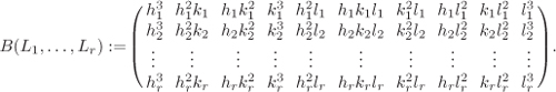, compute an elliptic curve ε defined over and points such that modulo p the curve ε reduces to E and the points S1, . . . , Sr to Rp,1, . . . , Rp,r. If the rank of ε is small, then the points S2, . . . , Sr are expected to be linearly dependent. Computing a non-trivial linear dependency among S2, . . . , Sr gives a linear dependency among Rp,1, . . . , Rp,r, which in turn yields indP Q with high probability. The details are now explained. For r points Li := [hi, ki, li], i = 1, . . . , r, we use the notation: [View full size image]

We start by fixing an integer r, 4 ≤ r ≤ 9. We then choose r random pairs (s_i, t_i) of integers and compute the points

We now apply a change of coordinates of the form

Equation 4.13

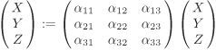
so that the first four of the points R_p,i become R_p,1 = [1, 0, 0], R_p,2 = [0, 1, 0], R_p,3 = [0, 0, 1] and R_p,4 = [1, 1, 1]. This change of coordinates fails if some three of the four points R_p,1, R_p,2, R_p,3 and R_p,4 sum to . But in that case the desired index ind_P Q can be computed with high probability. If, for example, , then we have (s₁ + s₂ + s₃)P = (t₁ + t₂ + t₃)Q and, therefore, if gcd(t₁ + t₂ + t₃, n) = 1, then ind_P Q ≡ (t₁ + t₂ + t₃)^–1(s₁ + s₂ + s₃) (mod n). On the other hand, if gcd(t₁ + t₂ + t₃, n) ≠ 1, we repeat with a different set of pairs (s_i, t_i).

Henceforth, we assume that the change of coordinates, as given in Equation (4.13), is successful. This transforms the equation for E to a general cubic equation:

C_p : u_p,1X³ + u_p,2X²Y + u_p,3XY² + u_p,4Y³ + u_p,5X²Z + u_p,6XY Z + u_p,7Y²Z + u_p,8XZ² + u_p,9Y Z² + u_p,10Z³ = 0.

Now, we carry out a step that heuristically ensures that the curve ε over (that we are going to construct) has a small rank. We choose a product M of small primes with p M, a cubic curve

C_M : u_M,1X³ + u_M,2X²Y + u_M,3XY² + u_M,4Y³ + u_M,5X²Z + u_M,6XYZ + u_M,7Y²Z + u_M,8XZ² + u_M,9Y Z² + u_M,10Z³ ≡ 0 (mod M)

over and points R_M,1, . . . , R_M,r on C_M and with coordinates in . The first four points should be R_M,1 = [1, 0, 0], R_M,2 = [0, 1, 0], R_M,3 = [0, 0, 1] and R_M,4 = [1, 1, 1]. We have to ensure also that for every prime divisor q of M, the matrix B(R_M,1, . . . , R_M,r) has maximal rank modulo q. In practice, it is easier to choose the points R_M,1, . . . , R_M,r first and then compute a curve C_M passing through these points by solving a set of linear equations in the coefficients u_M,1, . . . , u_M,10 of C_M. The curve C_M should be so chosen that it has the minimum possible number of solutions modulo M. This, in conjunction with some deep conjectures in the theory of elliptic curves, guarantees that the curve ε that we will construct shortly will have a rank less than the expected value.

We now combine the curves C_p and C_M as follows. Using the Chinese remainder theorem, we compute integers such that (mod p) and (mod M) for each i = 1, . . . , 10. Similarly, we compute points R₁, . . . , R_r with integer coefficients such that R_i ≡ R_p,i (mod p) and R_i ≡ R_M,i (mod M) for each i = 1, . . . , r, where congruence of points stands for coordinate-wise congruence. Here we have R₁ = [1, 0, 0], R₂ = [0, 1, 0], R₃ = [0, 0, 1] and R₄ = [1, 1, 1].

Clearly, the points R₁, . . . , R_r are lifts of the points R_p,1, . . . , R_p,r respectively, whereas the cubic curve

over is a lift of E. However, , treated as a curve over , need not pass through the points R₁, . . . , R_r. In order to ensure this last condition, we modify the coefficients of to the (small integer) coefficients u₁, . . . , u₁₀ by solving the system of linear equations

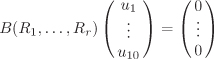
subject to the condition that (mod pM) for each i = 1, . . . , 10. The resulting cubic curve

C : u₁X³ + u₂X²Y + u₃XY² + u₄Y³ + u₅X²Z + u₆XYZ + u₇Y²Z + u₈XZ² + u₉Y Z² + u₁₀Z³ = 0

over evidently continues to be a lift of E.

Now, we apply a change of coordinates in order to transfer to the standard Weierstrass equation

ε : Y² + a₁XY + a₃Y = X³ + a₂X² + a₄X + a₆

with integer coefficients a_i. This transformation changes the points R₁, . . . , R_r to the points S₁, . . . , S_r. One should also ensure that .

Finally, we check if S₂, . . . , S_r are linearly dependent. If so, we determine a (non-trivial) relation with . This corresponds to the relation , where n₁ := –(n₂ + ··· + n_r), that is, sP = tQ with s := n₁s₁ + ··· + n_rs_r and t := n₁t₁ + ··· + n_rt_r. If gcd(t, n) = 1, we have ind_P Q ≡ t^–1s (mod n).

On the other hand, if S₂, . . . , S_r are linearly independent or if gcd(t, n) > 1, then the lifted data fail to compute ind_P Q. In that case, we repeat the entire process by selecting new pairs (s_i, t_i) and/or new points R_M,1, . . . , R_M,r.

This completes our description of the XCM. See Silverman [277] for further details. No rigorous or heuristic analysis of the running time of the XCM is available in the literature. Practical experience (reported in Jacobson et al. [139]) shows that the algorithm is rather impractical. The predominant cause for failure of a trial of the XCM is that the probability that the points S₂, . . . , S_r are linearly dependent is amazingly low. Suitable choices of the curve C_M help us to construct curves ε of low rank, but not low enough, in general, to render S₂, . . . , S_r linearly dependent. Larger values of r are expected to increase the probability of success in each trial, but it is not clear how to handle the values r > 9. Nevertheless, the XCM is a radically new idea to solve the ECDLP. As Joseph Silverman [277] says, “some of the ideas may prove useful in future work on ECDLP”.

Exercise Set 4.5

4.24	Let K be a field, and . Elements of μm are called the m-th roots of unity. Prove the following assertions. μm is a subgroup of (, ·). If char K = 0, then #μm = m. [H] If p := char K > 0, then #μm = m/pvp(m). [H] μm is cyclic. [H] The set is a subgroup of .
4.25	We use the notations of the last exercise and assume that #μm = m, that is, either char K = 0 or p := char K > 0 is coprime to m. In this case, a generator of μm is called a primitive m-th root of unity. If is a primitive m-th root of unity and ωr = 1 for some , then evidently m|r. In particular, m is the smallest of the exponents such that ωr = 1. The (monic) polynomial where the product runs over all primitive m-th roots of unity, is called the m-th cyclotomic polynomial (over K). Clearly, deg Φm(X) = φ(m) (where φ is Euler’s totient function). Show that . [H] Use the Möbius inversion formula to deduce that , where μ is the Möbius function. Conclude that . If m is a prime, show that Φm(X) = Xm–1 + ··· + X + 1. Let m ≠ 1 be odd and char K ≠ 2. Show that Φ2m(X) = Φm(–X). [H] Show that if , l is the (multiplicative) order of q modulo m and if ω is a primitive m-th root of unity, then [K(ω) : K] = l. [H] In particular, Φm is a product of φ(m)/l (distinct) irreducible polynomials each of degree l.
4.26	Let G be an (additive) Abelian group (not necessarily finite). Show that the subset is a subgroup of G. Gtors is called the torsion subgroup of G and the elements of Gtors are called torsion elements of G. An element is a torsion element of G if and only if a is of finite order. Let ε be an elliptic curve defined over a number field K. Show that the torsion subgroup εtors(K) of ε(K) is finite. [H] Let ε and K be as in Part (b). Show that is not finite. [H]