
Control Systems
Laplace transforms and the transfer function 13.2
Generally desirable and acceptable behaviour 13.5
Classification of system and static accuracy 13.7
Frequency-response methods 13.10
Some necessary mathematical preliminaries 13.13
The z transformation 13.13.1 13/25
Sampler and zero-order hold 13.14
Closed-loop systems 13.16 13/27
Stability 13.17 13/28
Example 13.18 13/28
Dead-beat response 13.19 13/30
Simulation 13.20 13/30
System models 13.20.1 13/30
Integration schemes 13.20.2 13/32
Organisation of problem input 13.20.3 13/32
Illustrative example 13.20.4 13/32
Multivariable control 13.21 13/33
Dealing with non-linear elements 13.22 13/35
Introduction 13.22.1 13/35
The describing function 13.22.2 13/35
State space and the phase plane 13.22.3 13/38
Disturbances 13.23 13/42
Ratio control 13.24 13/45
Transit delays 13.25 13/47
Introduction 13.25.1 13/47
The Smith predictor 13.25.2 13/48
Stability 13.26 13/48
Introduction 13.26.1 13/48
Definitions and performance criteria 13.26.2 13/48
Methods of stability analysis 13.26.3 13/51
Industrial controllers 13.27 13/52
Introduction 13.27.1 13/52
A commercial controller 13.27.2 13/52
Bumpless transfer 13.27.3 13/54
Integral windup and desaturation 13.27.4 13/54
Selectable derivative action 13.27.5 13/55
Variations on the PID algorithm 13.27.6 13/55
Incremental controllers 13.27.7 13/56
Scheduling controllers 13.27.8 13/56
Variable gain controllers 13.27.9 13/56
Inverse plant model 13.27.10 13/56
Digital control algorithms 13.28 13/57
Introduction 13.28.1 13/57
Shannon’s sampling theorem 13.28.2 13/58
Control algorithms 13.28.3 13/59
Auto-tuners 13.29 13/59
Practical tuning methods 13.30 13/60
Introduction 13.30.1 13/60
Ultimate cycle methods 13.30.2 13/61
Bang/bang oscillation test 13.30.3 13/61
Reaction curve test 13.30.4 13/61
A model building tuning method 13.30.5 13/62
General comments 13.30.6 13/63
13.1 Introduction
Examples of the conscious application of feedback control ideas have appeared in technology since very early times: certainly the float-regulator schemes of ancient Greece were notable examples of such ideas. Much later came the automatic direction-setting of windmills, the Watt governor, its derivatives, and so forth. The first third of the 1900s witnessed applications in areas such as automatic ship steering and process control in the chemical industry. Some of these later applications attracted considerable analytical effort aimed at attempting to account for the seemingly capricous dynamic behaviour that was sometimes found in practice.
However, it was not until during, and immediately after, World War II that the fundamentals of the above somewhat disjointed control studies were subsumed into a coherent body of knowledge which became recognised as a new engineering discipline. The great thrust in achieving this had its main antecedents in work done in the engineering electronics industry in the 1930s. Great theoretical strides were made and the concept of feedback was, for the first time, recognised as being all pervasive. The practical and theoretical developments emanating from this activity, constitute the classical approach to control which are explored in some detail in this chapter.
Since the late 1940s, tremendous efforts have been made to expand the boundaries of control engineering theory. For example, ideas from classical mechanics and the calculus of variations have been adapted and extended from a control-theoretic viewpoint. This work is based largely on the state-space description of systems (this description is briefly described in Section 13.11). However, it must be admitted that the practical uses and advantages of many of these developments have yet to be demonstrated. Most control system design work is still based on the classical work mentioned previously. Moreover, nowadays these applications rely, very heavily, on the use of computer techniques; indeed, computers are commonly used as elements in control loops.
Techniques from the ‘classical’ period of control engineering development is easily understood, wide-ranging in application and, perhaps most importantly, capable of coping with deficiencies in detailed knowledge about the system to be controlled.
These techniques are easily adapted for use in the computer-aided design of control systems, and have proved themselves capable of extension into the difficult area of multi-variable system control; however, this latter topic is beyond the scope of this chapter. So with the above comments in mind, a conventional basic approach to control theory is presented, with a short discussion of the state-space approach and a more extensive forage into sampled-data systems. These latter systems have become important owing to the incorporation of digital computers, particularly microcomputers, into the control loop. Fortunately, an elementary theory for sampled data can be established which nicely parallels the development of basic continuous control theory.
The topics covered in this introduction, and extensions of them, have stood practitioners in good stead for several decades now, and can be confidently expected to go on delivering good service for some decades to come.
13.2 Laplace transforms and the transfer function
In most engineering analysis it is usual to produce mathematical models (of varying precision) to predict the behaviour of physical systems. Often such models are manifested by a differential equation description. This appears to fit in with the causal behaviour of idealised components, e.g. Newton’s law relating the second derivative of displacement to the applied force. It is possible to model such behaviour in other ways (for example, using integral equations), although these are much less familiar to most engineers. All real systems are non-linear; however, it is fortuitous that most systems behave approximately like linear ones, with the implication that superposition holds true to some extent. We further restrict the coverage here in that we shall be concerned particularly with systems whose component values are not functions of time—at least over the time-scale of interest to us.
In mathematical terms this latter point implies that the resulting differential equations are not only linear, but also have constant coefficients, e.g. many systems behave approximately according to the equation
where x is the dependent variable (displacement, voltage, etc.), f(t) is a forcing function (force, voltage source, etc.), and ωn2 and ζ are constants the values of which depend on the size and interconnections of the individual physical components making up the system (spring-stiffness constant, inductance values, etc.).
Equations having the form of Equation (13.1) are called ‘linear constant coefficient ordinary differential equations’ (LCCDE) and may, of course, be of any order. There are several techniques available for solving such equations but the one of particular interest here is the method based on the Laplace transformation. This is treated in detail elsewhere, but it is useful to outline the specific properties of particular interest here.
13.2.1 Laplace transformation
Given a function f(t), then its Laplace transformation F(s) is defined as
where, in general, s is a complex variable and of such a magnitude that the above integral converges to a definite functional value.
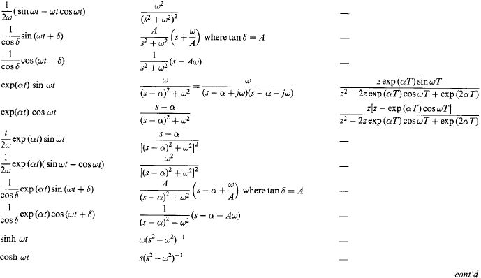
A list of Laplace transformation pairs is given in Table 13.1.
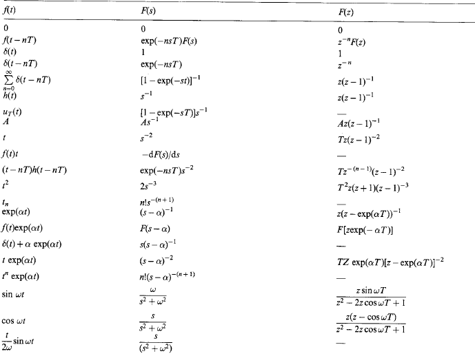
The essential usefulness of the Laplace transformation technique in control engineering studies is that it transforms LCCDE and integral equations into algebraic ones and, hence, makes for easier and standard manipulation.
13.2.2 The transfer function
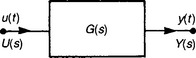
This is a central notion in control work and is, by definition, the Laplace transformation of the output of a system divided by the Laplace transformation of the input, with the tacit assumption that all initial conditions are at zero.
Thus, in Figure 13.1, where y(t) is the output of the system and u(t) is the input, then the transfer function G(s) is
Supposing that y(t) and u(t) are related by the general LCCDE
then, on Laplace transforming and ignoring initial conditions, we have (see later for properties of Laplace transformation)
There are a number of features to note about G(s).
(1) Invariably n>m for physical systems.
(2) It is a ratio of two polynomials which may be written
z1, …, zm are called the zeros and p1, …, pn are called the poles of the transfer function.
(3) It is not an explicit function of input or output, but depends entirely upon the nature of the system.
(4) The block diagram representation shown in Figure 13.1 may be extended so that the interaction of composite systems can be studied (provided that they do not load each other); see below.
(5) If u(t) is a delta function δ(t), then U(s) = 1, whence Y(s) = G(s) and y(t) = g(t), where g(t) is the impulse response (or weighting function) of the system.
(6) Although a particular system produces a particular transfer function, a particular transfer function does not imply a particular system, i.e. the transfer function specifies merely the input—output relationship between two variables and, in general, this relationship may be realised in an infinite number of ways.
(7) Although we might expect that all transfer functions will be ratios of finite polynomials, an important and common element which is an exception to this is the pure-delay element. An example of this is a loss-free transmission line in which any disturbance to the input of the line will appear at the output of the line without distortion, a finite time (say τ) later. Thus, if u(t) is the input, then the output y(t) = u(t − τ) and the transfer function Y(s)/U(s) = exp(−sτ). Hence, the occurrence of this term within a transfer function expression implies the presence of a pure delay; such terms are common in chemical plant and other fluid-flow processes.
Having performed any manipulations in the Laplace transformation domain, it is necessary for us to transform back to the time domain if the time behaviour is required. Since we are dealing normally with the ratio of polynomials, then by partial fraction techniques we can arrange Y(s) to be written in the following sequences:
and by so arranging Y(s) in this form the conversion to y(t) can be made by looking up these elemental forms in Table 13.1.
13.2.3 Certain theorems
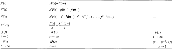
A number of useful transform theorems are quoted below, without proof.
If F(s) is the Laplace transformation of f(t), then
For example, if f(t) = exp(−bt), then
Repeated integration follows in a similar fashion.
If f(t) and f′(t) are Laplace transformable and if L[f(t)] = F(s), then if the limit of f(t) exists as t goes towards infinity, then
If f(t) and f′(t) are Laplace transformable and if L[f(t)] = F(s),
13.3 Block diagrams
It is conventional to represent individual transfer functions by boxes with an input and output (see note (4) in Section 13.2.2). Provided that the components represented by the transfer function do not load those represented by the transfer function in a connecting box, then simple manipulation of the transfer functions can be carried out. For example, suppose that there are two transfer functions in cascade (see Figure 13.2): then we may write X(s)/U(s) = G1(s) and Y(s)/X(s) = G2(s). Eliminating X(s) by multiplication, we have
which may be represented by a single block. This can obviously be generalised to any number of blocks in cascade.
Another important example of block representation is the prototype feedback arrangement shown in Figure 13.3. We see that Y(s) = G(s)E(s) and E(s) = U(s) − H(s) Y(s). Eliminating E(s) from these two equations results in
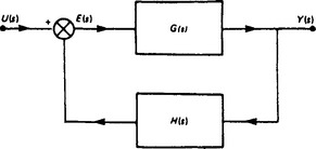
In block diagram form we have Figure 13.4. If we eliminate Y(s) from the above equations, we obtain
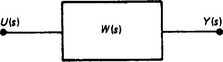
Figure 13.4 Reduction of the diagram shown in Figure 13.3 to a single block
13.4 Feedback
The last example is the basic feedback conceptual arrangement, and it is pertinent to investigate it further, as much effort in dealing with control systems is devoted to designing such feedback loops. The term ‘feedback’ is used to describe situations in which a portion of the output (and/or processed parts of it) are fed back to the input of the system. The appropriate application may be used, for example, to improve bandwidth, improve stability, improve accuracy, reduce effects of unwanted disturbances, compensate for uncertainty and reduce the sensitivity of the system to component value variation.
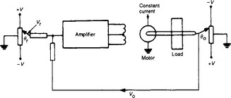
As a concrete example consider the system shown in Figure 13.5, which displays the arrangements for an angular position control system in which a desired position θr is indicated by tapping a voltage on a potentiometer. The actual position of the load being driven by the motor (usually via a gearbox) is monitored by θo, indicated, again electrically, by a potentiometer tapping. If we assume identical potentiometers energised from the same voltage supply, then the misalignment between the desired output and the actual output is indicated by the difference between the respective potentiometer voltages. This difference (proportional to error) is fed to an amplifier whose output, in turn, drives the motor. Thus, the arrangement seeks to drive the system until the output θo and input θr are coincident (i.e. the error is zero).
In the more general block diagram form, the above schematic will be transformed to that shown in Figure 13.6, where θr(s), θo(s) are the Laplace transforms of the input, output position: K1(s) and K2(s) are the potentiometer transfer functions (normally taken as straight gains); Vr(s) is the Laplace transform of the reference voltage; Vo(s) is the Laplace transform of the output voltage; Gm(s) is the motor transfer function; G1(s) is the load transfer function; and A(s) is the amplifier transfer function.
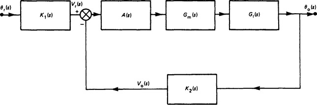
Figure 13.6 Block diagram of the system shown in Figure 13.5
Let us refer now to Figure 13.3 in which U(s) is identified as the transformed input (reference or demand) signal, Y(s) is the output signal and E(s) is the error (or actuating) signal. G(s) represents the forward transfer function and is the product of all the transfer functions in the forward loop, i.e. G(s) = A(s)Gm(s)G1(s) in the above example.
H(s) represents the feedback transfer function and is the product of all transfer functions in the feedback part of the loop.
We saw in Section 13.3 that we may write
i.e. we have related output to input and the error to the input.
The product H(s)G(s) is called the open-loop transfer function and G(s)/[1+H(s)G(s)] the closed-loop transfer function. The open-loop transfer function is most useful in studying the behaviour of the system, since it relates the error to the demand. Obviously it would seem desirable for this error to be zero at all times, but since we are normally considering systems containing energy storage components, total elimination of error at all times is impossible.
13.5 Generally desirable and acceptable behaviour
Although specific requirements will normally be drawn up for a particular control system, there are important general requirements applicable to the majority of systems. Usually an engineering system will be assembled from readily available components to perform some function, and the choice of these components will be restricted. An example of this would be a diesel engine–alternator set for delivering electrical power, in which normally the most convenient diesel engine–alternator combination will be chosen from those already manufactured.
Even if such a system were assembled from customer-designed components, it would be fortuitous if it performed in a satisfactory self-regulatory way without further consideration of its control dynamics. Hence, it is the control engineer’s task to take such a system and devise economical ways of making the overall system behave in a satisfactory manner under the expected operational conditions.
For example, a system may oscillate, i.e. it is unstable; or, although stable, it might tend to settle after a change in input demand to a value unacceptably far from this new demand, i.e. it lacks static accuracy. Again, it might settle to a satisfactory new steady state, but only after an unsatisfactory transient response. Alternatively, normal operational load disturbances on the system may cause unacceptably wide variation of the output variable, e.g. voltage and frequency of the engine—alternator system.
All these factors will normally be quantified in an actual design specification, and fortunately a range of techniques is available for improving the behaviour. But the application of a particular technique to improve the performance of one aspect of behaviour often has a deleterious effect on another, e.g. improved stability with improved static accuracy tends to be incompatible. Thus, a compromise is sought which gives the ‘best’ acceptable all-round performance. We now discuss some of these concepts and introduce certain techniques useful in examining and designing systems.
13.6 Stability
This is a fairly easy concept to appreciate for the types of system under consideration here. Equation (13.2) with the right-hand side made equal to zero governs the free (or unforced, or characteristic) behaviour of the system, and because of the nature of the governing LCCDE it is well known that the solution will be a linear combination of exponential terms, viz.
where the αi values are the roots of the so-called ‘characteristic equation’.
It will be noted that should any αi have a positive real part (in general, the roots will be complex), then any disturbance will grow in time. Thus, for stability, no roots must lie in the right-hand half of the complex plane or s plane. In a transfer function context this obviously translates to ‘the roots of the denominator must not lie in the right-hand half of the complex plane’.
For example, if W(s) = G(s)/[1+H(s)G(s)], then the roots referred to are those of the equation
In general, the determination of these roots is a non-trivial task and, as at this stage we are interested only in whether the system is stable or not, we can use certain results from the theory of polynomials to achieve this without the necessity for evaluating the roots.
A preliminary examination of the location of the roots may be made using the Descartes rule of signs, which states: if f(x) is a polynomial, the number of positive roots of the equation f(x) = 0 cannot exceed the number of changes of sign of the numerical coefficients of f(x), and the number of negative roots cannot exceed the number of changes of sign of the numerical coefficients of f(−x). ‘A change of sign’ occurs when a term with a positive coefficient is immediately followed by one with a negative coefficient, and vice versa.
Example Suppose that f(x) = x3+3x − 2 = 0; then there can be at most one positive root. Since f(−x) = −x3 − 3x − 2, the equation has no negative roots. Further, the equation is cubic and must have at least one real root (complex roots occur in conjugate pairs); therefore the equation has one positive-real root.
Although Descartes’ result is easily applied, it is often indefinite in establishing whether or not there is stability, and a more discriminating test is that due to Routh, which we give without proof.
Suppose that we have the polynomial
where all coefficients are positive, which is a necessary (but not sufficient) condition for the system to be stable, and we construct the following so-called ‘Routh array’:
This array will have n+1 rows.
If the array is complete and none of the elements in the first column vanishes, then a sufficient condition for the system to be stable (i.e. the characteristic equation has all its roots with negative-real parts) is for all these elements to be positive. Further, if these elements are not all positive, then the number of changes of sign in this first column indicates the number of roots with positive-real parts.
Example Determine whether the polynomial s4+2s3+6s2+7s+4 = 0 has any roots with positive-real parts. Construct the Routh array:
There are five rows with the first-column elements all positive, and so a system with this polynomial as its characteristic would be stable.
There are cases that arise which need a more delicate treatment.
(1) Zeros occur in the first column, while other elements in the row containing a zero in the first column are non-zero.
In this case the zero is replaced by a small positive number, ε, which is allowed to approach zero once the array is complete.
For example, consider the polynomial equation
Thus, α1 is a large negative number and we see that there are effectively two changes of sign and, hence, the equation has two roots which lie in the right-hand half of this plane.
(2) Zeros occur in the first column and other elements of the row containing the zero are also zero.
This situation occurs when the polynomial has roots that are symmetrically located about the origin of the s plane, i.e. it contains terms such as (s+jω)(s − jω) or (s+v)(s − v).
This difficulty is overcome by making use of the auxiliary equation which occurs in the row immediately before the zero entry in the array. Instead of the all-zero row the equation formed from the preceding row is differentiated and the resulting coefficients are used in place of the all-zero row.
For example, consider the polynomial s3+3s2+2s+6 = 0.
Differentiate the auxiliary equation giving 6s = 0, and compile a new array using the coefficients from this last equation, viz.
Since there are no changes of sign, the system will not have roots in the right-hand half of the s plane.
Although the Routh method allows a straightforward algorithmic approach to determining the stability, it gives very little clue as to what might be done if stability conditions are unsatisfactory. This consideration is taken up later.
13.7 Classification of system and static accuracy
The discussion in this section is restricted to unity-feedback systems (i.e. H(s) = 1) without seriously affecting generalities. We know that the open-loop system has a transfer function KG(s), where K is a constant and we may write
and for physical systems n ≥ m+1.
The order of the system is defined as the degree of the polynomial in s appearing in the denominator, i.e. n.
The rank of the system is defined as the difference in the degree of the denominator polynomial and the degree of the numerator polynomial, i.e. n − m ≥ 1.
The class (or type) is the degree of the s term appearing in the denominator (i.e. l), and is equal to the number of integrators in the system.
13.7.2 Static accuracy
When a demand has been made on the system, then it is generally desirable that after the transient conditions have decayed the output should be equal to the input. Whether or not this is so will depend both on the characteristics of the system and on the input demand. Any difference between the input and output will be indicated by the error term e(t) and we know that for the system under consideration
Let ess = limt-∞ e(t) (if it exists), and so ess will be the steady-state error. Now from the final-value theorem we have
13.7.2.1 Position-error coefficient Kp
Suppose that the input is a unit step, i.e. R(s) = 1/s; then
where Kp = lims→0[KG(s)] and this is called the position-error coefficient.
Therefore Kp = K(b0/a0) and ess = 1/(1+Kp).
It will be noted that, after the application of a step, there will always be a finite steady-state error between the input and the output, but this will decrease as the gain K of the system is increased.
i.e. there is no steady-state error in this case and we see that this is due to the presence of the integrator term 1/s. This is an important practical result, since it implies that steady-state errors can be eliminated by use of integral terms.
13.7.2.2 Velocity-error coefficient, Kv
Let us suppose that the input demand is a unit ramp, i.e. u(t) = t, so U(s) = 1/s2. Then
where Kv = lims→0[sKG(s)] is called the velocity-error coefficient.
Examples For a type-0 system Kv = 0, whence ess → ∞.
For a type-1 system Kv = K(b0/a0) and so this system can follow but with a finite error.
whence ess → 0 and so the system can follow in the steady state without error.
13.7.2.3 Acceleration-error coefficient Ka
In this case we assume that u(t) = t2/2, so U(s) = 1/s3 and so
where Ka = lims→0[s2 KG(s)] is called the acceleration-error coefficient and similar analyses to the above may be performed.
These error-coefficient terms are often used in design specifications of equipment and indicate the minimum order of the system that one must aim to design.
13.7.3 Steady-state errors due to disturbances
The prototype unity-feedback closed-loop system is shown in Figure 13.7 modified by the intrusion of a disturbance D(s) being allowed to affect the loop. For example, the loop might represent a speed-control system and D(s) might represent the effect of changing the load. Now, since linear systems are under discussion, in order to evaluate the effects of this disturbance on Y(s) (denoted by YD(s)), we may tacitly assume U(s) = 0 (i.e. invoke the superposition principle)
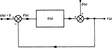
Now ED(s) = −YD(s) = −D(s)/[1+KG(s)], and so the steady-state error, essD due to the application of the disturbance, may be evaluated by use of the final-value theorem as
Obviously the disturbance may enter the loop at other places but its effect may be established by similar analysis.
13.8 Transient behaviour
Having developed a means of assessing stability and steady-state behaviour, we turn our attention to the transient behaviour of the system.
13.8.1 First-order system
It is instructive to examine first the behaviour of a first-order system (a first-order lag with a time constant T) to a unit-step input (Figure 13.8).
note also that dy/dt = (1/T) exp(−t/T).
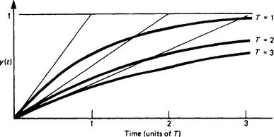
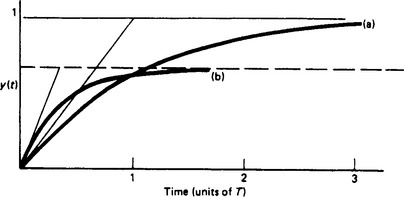
Figure 13.8 shows this time response for different values of T where it will be noted that the corresponding trajectories have slopes of 1/T at time t = 0 and reach approximately 63% of their final values after T.
Suppose now that such a system is included in a unity-feedback arrangement together with an amplifier of gain K (Figure 13.9); therefore
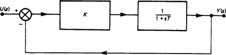
For a unit-step input the time response will be
This expression has the same form as that obtained for the open loop but the effective time constant is modified by the gain and so is the steady-state condition (Figure 13.10). Such an arrangement provides the ability to control the effective time constant by altering the gain of an amplifier, the original physical system being left unchanged.
13.8.2 Second-order system
The behaviour characteristics of second-order systems are probably the most important of all, since many systems of seemingly greater complexity may often be approximated by a second-order system because certain poles of their transfer function dominate the observed behaviour. This has led to system specifications often being expressed in terms of second-order system behavioural characteristics.
In Section 13.2 the importance of the second-order behaviour of a generator was mentioned, and this subject is now taken further by considering the system shown in Figure 13.11.
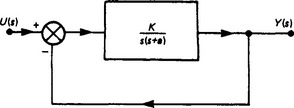
The closed-loop transfer function for this system is given by
and this may be rewritten in general second-order terms in the form
where ![]() and
and ![]() . The unit-step response is given by
. The unit-step response is given by
where ![]() . This assumes, of course, that ζ, < 1, so giving an oscillating response decaying with time.
. This assumes, of course, that ζ, < 1, so giving an oscillating response decaying with time.
The rise time tr will be defined as the time to reach the first overshoot (note that other definitions are used and it is important to establish which particular definition is being used in a particular specification):
i.e. the rise time decreases as the gain K is increased.
The percentage overshoot is defined as:
i.e. the percentage overshoot increases as the gain K increases.
The frequency of oscillation ωr is immediately seen to be
i.e. the frequency of oscillation increases as the gain K increases.
The predominant time constant is the time constant associated with the envelope of the response (Figure 13.12) which is given by exp(–ζωnt) and thus the predominant time constant is 1/ζωn:
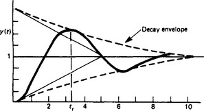
Figure 13.12 Step response of the system shown in Figure 13.11. The rise time tr is the time taken to reach maximum overshoot. The predominant time constant is indicated by the tangents to the envelope curve
Note that this time constant is unaffected by the gain K and is associated with the ‘plant parameter a’, which will normally be unalterable, and so other means must be found to alter the predominant time constant should this prove necessary.
The settling time ts is variously defined as the time taken for the system to reach 2–5% (depending on specification) of its final steady state and is approximately equal to four times the predominant time constant.
It should be obvious from the above that characteristics desired in plant dynamical behaviour may be conflicting (e.g. fast rise time with small overshoot) and it is up to the skill of the designer to achieve the best compromise. Overspecification can be expensive.
A number of the above items can be directly affected by the gain K and it may be that a suitable gain setting can be found to satisfy the design with no further attention. Unfortunately, the design is unlikely to be as simple as this, in view of the fact that the predominant time constant cannot be influenced by K. A particularly important method for influencing this term is the incorporation of so-called velocity feedback.
13.8.3 Velocity feedback
Given the prototype system shown in Figure 13.11, suppose that this is augmented by measuring the output y(t), differentiating to form ![]() , and feeding back in parallel with the normal feedback a signal proportional to
, and feeding back in parallel with the normal feedback a signal proportional to ![]() : say
: say ![]() . The schematic of this arrangement is shown in Figure 13.13. Then, by simple manipulation, the modified transfer function becomes
. The schematic of this arrangement is shown in Figure 13.13. Then, by simple manipulation, the modified transfer function becomes
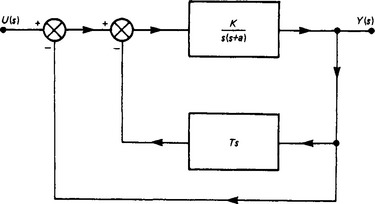
whence the modified predominant time constant is given by 2/(a+TK). The designer effectively has another string to his bow in that manipulation of K and T is normally very much in his command.
A similar effect may be obtained by the incorporation of a derivative term to act on the error signal (Figure 13.14) and in this case the transfer function becomes
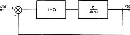
It may be demonstrated that this derivative term when correctly adjusted can both stabilise the system and increase the speed of response. The control shown in Figure 13.14 is referred to as proportional-plus-derivative control and is very important.
13.8.4 Incorporation of integral control
Mention has previously been made of the effect of using integrators within the loop to reduce steady-state errors; a particular study with reference to input/output effects was given. In this section consideration is given to the effects of disturbances injected into the loop, and we consider again the simple second-order system shown in Figure 13.11 but with a disturbance occurring between the amplifier and the plant dynamics. Appealing to superposition we can, without loss of generality, put U(s) = 0 and the transfer function between the output and the disturbance is then given by
Assuming that d(t) is a unit step, D(s) = 1/s, and using the final-value theorem, limt→∞y(t) is obtained from
and so the effect of this disturbance will always be present. By incorporating an integral control as shown in Figure 13.15, the output will, in the steady state, be unaffected by the disturbance, viz.
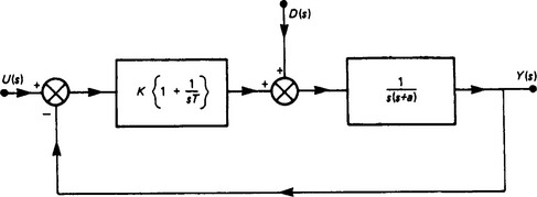
This controller is called a proportional-plus-integral controller.
An unfortunate side-effect of incorporating integral control is that it tends to destabilise the system, but this can be minimised by careful choice of T. In a particular case it might be that proportional-plus-integral-plus-derivative (PID) control may be called for, the amount of each particular control type being carefully proportioned.
In the foregoing discussions we have seen, albeit by using specific simple examples, how the behaviour of a plant might be modified by use of certain techniques. It is hoped that this will leave the reader with some sort of feeling for what might be done before embarking on more general tools, which tend to appear rather rarefied and isolated unless a basic physical feeling for system behaviour is present.
13.9 Root-locus method
The root locus is merely a graphical display of the variation of the poles of the closed-loop system when some parameter, often the gain, is varied. The method is useful since the loci may be obtained, at least approximately, by straightforward application of simple rules, and possible modification to reshape the locus can be assessed.
Considering once again the unity-feedback system with the open-loop transfer function KG(s) = Kb(s)/a(s), where b(s) and a(s) represent m th- and n th-order polynomials, respectively, and n>m, then the closed-loop transfer function may be written as
Note that the system is n th order and the zeros of the closed loop and the open loop are identical for unity feedback. The characteristic behaviour is determined by the roots of 1+KG(s) = 0 or a(s)+Kb(s) = 0. Thus, G(s) = −(1/K) or b(s)/a(s) = −(1/K).
Let sr be a root of this equation; then
where n may take any integer value, including n = 0. Let z1, …, zm be the roots of the polynomial b(s) = 0, and p1, …, pn be the roots of the polynomial a(s) = 0. Then
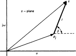
Now, given a complex number pj, the determination of the complex number (s − pj), where s is some point in the complex plane, is illustrated in Figure 13.16, where the mod(s − pj) and phase (s − pj) are also illustrated. The determination of the magnitudes and phase angles for all the factors in the transfer function, for any s, can therefore be done graphically.
The complete set of all values of s, constituting the root locus may be constructed using the angle condition alone; once found, the gain K giving particular values of sr may be easily determined from the magnitude condition.
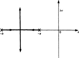
Example Suppose that G(s) = K/[(s+a)(s+b)], then it is fairly quickly established that the only sets of points satisfying the angle condition
are on the line joining −a to −b and the perpendicular bisector of this line (Figure 13.17).
13.9.1 Rules for construction of the root locus
(1) The angle condition must be obeyed.
(2) The magnitude condition enables calibration of the locus to be carried out.
(3) The root locus on the real axis must be in sections to the left of an odd number of poles and zeros. This follows immediately from the angle condition.
(4) The root locus must be symmetrical with respect to the horizontal real axis. This follows because complex roots must appear as complex conjugate pairs.
(5) Root loci always emanate from the poles of the open-loop transfer function where K = 0. Consider a(s)+Kb(s) = 0; then a(s) = 0 when K = 0 and the roots of this polynomial are the poles of the open-loop transfer function. Note that this implies that there will be n branches of the root locus.
(6) m of the branches will terminate at the zeros for K→∞. Consider a(s)+Kb(s) = 0, or (1/K)a(s)+b(s) = 0, whence as K→∞, b(s)→0 and, since this polynomial has m roots, these are where m of the branches terminate. The remaining n − m branches terminate at infinity (in general, complex infinity).
(7) These n − m branches go to infinity along asymptotes inclined at angles φi to the real axis, where
Consider a root sr approaching infinity, (sr − a) → sr for all finite values of a. Thus, if φi is the phase sr, then each pole and each zero term of the transfer function term will contribute approximately φi and − φi, respectively. Thus,
(8) The centre of these asymptotes is called the ‘asymptote centre’ and is (with good accuracy) given by
This can be shown by the following argument. For very large values of s we can consider that all the poles and zeros are situated at the point σA on the real axis. Then the characteristic equation (for large values of s) may be written as
or approximately, by using the binomial theorem,
Also, the characteristic equation may be written as
Expanding this for the first two terms results in
(9) When a locus breaks away from the real axis, it does so at the point where K is a local maximum. Consider the characteristic equation 1+K[b(s)/a(s)] = 0; then we can write K = p(s), where p(s) = −[a(s)/b(s)]. Now, where two poles approach each other along the real axis they will both be real and become equal when K has the maximum value that will enable them both to be real and, of course, coincident. Thus, an evaluation of K around the breakaway point will rapidly reveal the breakaway point itself.
Example Draw the root locus for
Procedure (Figure 13.18):
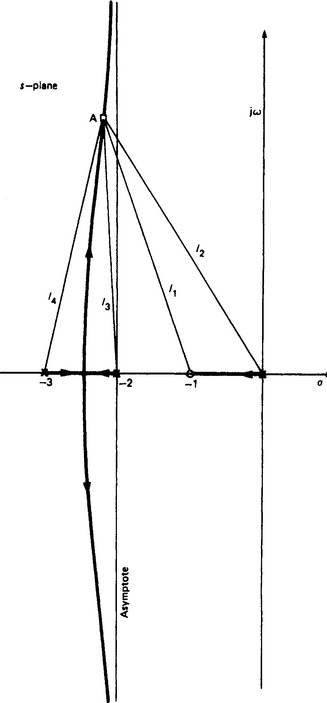
(1) Plot the poles of the open-loop system (i.e. at s = 0, s = −2, s = −3).
(2) Plot the zeros of the system (i.e. at z = −1).
(3) Determine the sections on the real axis at which closed-loop poles can exist. Obviously these are between 0 and −1 (this root travels along the real axis between these values as K goes from 0 → ∞), and between −2 and −3 (two roots are moving towards each other as K increases and, of course, will break away).
(7) Modulus. For a typical root situated at, for example, point A, the gain is given by K = l2l3l4/l1.
After a little practice the root locus can be drawn very rapidly and compensators can be designed by pole-zero placement in strategic positions. A careful study of the examples given in the table will reveal the trends obtainable for various pole-zero placements.
13.10 Frequency-response methods
Frequency-response characterisation of systems has led to some of the most fruitful analysis and design methods in the whole of control system studies. Consider the situation of a linear, autonomous, stable system, having a transfer function G(s), and being subjected to a unit-magnitude sinusoidal input signal of the form exp (jωt), starting at t = 0. The Laplace transformation of the resulting output of the system is
and the time domain solution will be
Since a stable system has been assumed, then the effects of the terms in the parentheses will decay away with time and so, after a sufficient lapse of time, the steady-state solution will be given by
The term G(jω), obtained by merely substituting jω for s in the transfer function form, is termed the frequency-response function, and may be written
where |G(jω)| = mod G(jω) and ∠G(jω) = phase G(jω). This implies that the output of the system is also sinusoidal in magnitude |G(jω)| with a phase-shift of ∠G(jω) with reference to the input signal.
Example Consider the equation of motion
where φ = arctan bω/(k − mω2).
Within the area of frequency-response characterisation of systems three graphical techniques have been found to be particularly useful for examining systems and are easily seen to be related to each other. These techniques are based upon:
(1) The Nyquist plot, which is the locus of the frequency-response function plotted in the complex plane using ω as a parameter. It enables stability, in the closed-loop condition, to be assessed and also gives an indication of how the locus might be altered to improve the behaviour of the system.
(2) The Bode diagram, which comprises two plots, one showing the amplitude of the output frequency response (plotted in decibels) against the frequency ω (plotted logarithmically) and the other of phase angle θ of the output frequency response plotted against the same abscissa.
(3) The Nichols chart, a direct plot of amplitude of the frequency response (again in decibels) against the phase angle, with frequency ω as a parameter, but further enables the closed-loop frequency response to be read directly from the chart.
In each of these cases it is the open-loop steady-state frequency response, i.e. G(jω), which is plotted on the diagrams.
13.10.1 Nyquist plot
The closed-loop transfer function is given by
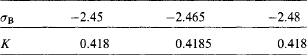
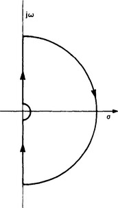
and the stability is determined by the location of the roots of 1+H(s)G(s) = 0, i.e. for stability no roots must have positive-real parts and so must not lie on the positive-real half of the complex plane. Assume that the open-loop transfer function H(s)G(s) is stable and consider the contour C, the so-called ‘Nyquist contour’ shown in Figure 13.19, which consists of the imaginary axis plus a semicircle of large enough radius in the right half of the s plane such that any zeros of 1+H(s)G(s) will be contained within this contour. This contour Cn is mapped via 1+H(s)G(s) into another curve γ into the complex plane s′. It follows immediately from complex variable theory that the closed loop will be stable if the curve γ does not encircle the origin in the s′ plane and unstable if it encircles the origin or passes through the origin. This result is the basis of the celebrated Nyquist stability criterion. It is rather more usual to map not 1+H(s)G(s) but H(s)G(s); in effect this is merely a change of origin from (0, 0) to (−1, 0), i.e. we consider curve γ′n.
Figure 13.19 Illustration of Nyquist mapping: (a) mapping contour on the s plane; (b) resulting mapping of 1+H(s)G(s) = 0 and the shift of the origin
The statement of the stability criterion is that the closed-loop system will be stable if the mapping of the contour Cn by the open-loop frequency-response function H(jω)G(jω) does not enclose the so-called critical point (−1, 0). Actually further simplification is normally possible, for:
(1) |H(s)G(s)| → 0 as |s| → ∞, so that the very large semicircular boundary maps to the origin in the s; plane.
(2) H(−jω)G(−jω) is the complex conjugate of H(jω)G(jω) and so the mapping of H(−jω)G(−jω) is merely the mirror image of H(jω)G(jω) in the real axis.
(3) Note: H(jω)G(jω) is merely the frequency-response function of the open loop and may even be directly measurable from experiments. Normally we are mostly interested in how this behaves in the vicinity of the (−1, 0) point and, therefore, only a limited frequency range is required for assessment of stability.
The mathematical mapping ideas stated above are perhaps better appreciated practically by the so-called left-hand rule for an open-loop stable system, which reads as follows: if the open-loop sinusoidal response is traced out going from low frequencies towards higher frequencies, the closed loop will be stable if the critical point (-1, 0) lies on the left of all points on H(jω)G(jω). If this plot passes through the critical point, or if the critical point lies on the right-hand side of H(jω)G(jω), the closed loop will be unstable.
If the open loop has poles that actually lie on the imaginary axis, e.g. integrator 1/s, then the contour is indented as shown in Figure 13.20 and the above rule still applies to this modification.
13.10.1.1 Relative stability criteria
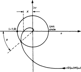
Obviously the closer the H(jω)G(jω) locus approaches the critical point, the more critical is the consideration of stability, i.e. we have an indication of relative stability, given a measure by the gain and phase margins of the system.
If the modulus of H(jω)G(jω) = X with a phase shift of 180°, then the gain margin is defined as
The gain margin is usually specified in decibels, where we have
Gain margin (dB) = 20 log(1/X) = −20 log X
The phase margin is the angle which the line joining the origin to the point on the open-loop response locus corresponding to unit modulus of gain makes with the negative-real axis. These margins are probably best appreciated diagrammatically (Figure 13.21). They are useful, since a rough working rule for reasonable system damping and stability is to shape the locus so that a gain margin of at least 6 dB is achieved and a phase margin of about 40°.
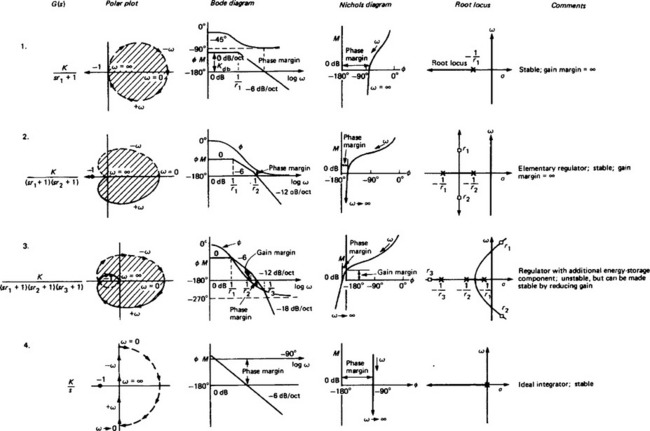
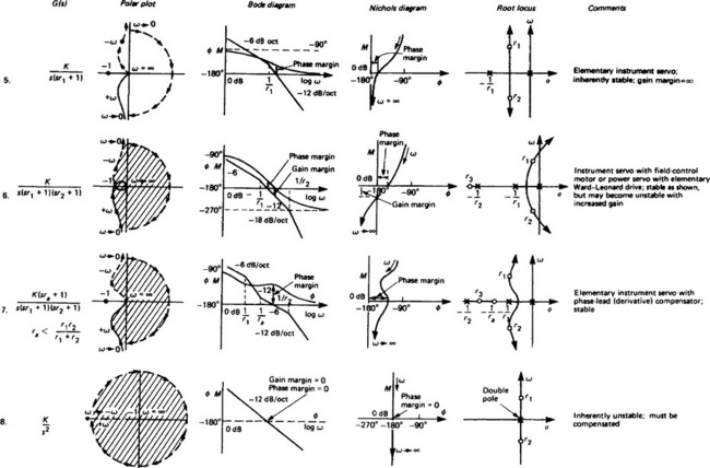
Examples of the Nyquist plot are shown in Figure 13.22. Although from such plots the modifications necessary to achieve more satisfactory performance can be easily appreciated, precise compensation arrangements are not easily determined, since complex multiplication is involved and an appeal to the Bode diagram can be more valuable.
13.10.2 Bode diagram
As mentioned above, the Bode diagram is a logarithmic presentation of the frequency response and has the advantage over the Nyquist diagram that individual factor terms may be added rather than multiplied, the diagram can usually be quickly sketched using asymptotic approximations and several decades of frequency may be easily considered.
i.e. the composite transfer function may be thought of as being composed of a number of simpler transfer functions multiplied together, so
This is merely each individual factor (in decibels) being added algebraically to a grand total. Further,
i.e. the individual phase shift at a particular frequency may be added algebraically to give the total phase shift.
It is possible to construct Bode diagrams from elemental terms including gain (K), differentiators and integrators (s and 1/s), lead and lag terms ((as+1) and (1+as)−1), quadratic lead and lag terms ((bs2+cs+1) and (bs2+cs+1)−1), and we consider the individual effects of their presence in a transfer function on the shape of the Bode diagram.
(a) Gain term, K The gain in decibels is simply 20 log K and is frequency independent; it merely raises (or lowers) the combined curve 20 log K dB.
(b) Integrating term, 1/s Now |G(jω)| = 1/ω and ∠G(jω) = −90° (a constant) and so the gain in decibels is given by 20 log(1/ω) = −20 log ω. On the Bode diagram this corresponds to a straight line with slope −20 dB/decade (or −6 dB/octave) of frequency and passes through 0 dB at ω = 1 (see plot 4 in Figure 13.22).
(c) Differentiating term, s Now |G(jω)| = ω and ∠G(jω) = 90° (a constant) and so the gain in decibels is given by 20 log ω. On the Bode diagram this corresponds to a straight line with slope 20 dB/decade of frequency and passes through 0 dB at ω = 1.
(d) First-order lag term, (1+Sτ)−1 The gain in decibels is given by
and the phase angle is given by ∠G(jω) = −tan−1 ωτ. When ω2τ2 is small compared with unity, the gain will be approximately 0 dB, and when ω2τ2 is large compared with unity, the gain will be −20 log ωτ. With logarithmic plotting this specifies a straight line having a slope of −20 dB/decade of frequency (6 dB/octave) intersecting the 0 dB line at ω = 1/τ. The actual gain at ω = 1/τ is −3 dB and so the plot has the form shown in plot 1 of Figure 13.22. The frequency at which ω = 1/τ is called the corner or break frequency. The two straight lines, i.e. those with 0 dB and −20 dB/decade, are called the ‘asymptotic approximations’ to the Bode plot. These approximations are often good enough for not too demanding design purposes.
The phase plot will lag a few degrees at low frequencies and fall to −90° at high frequency, passing through −45° at the break frequency.
(e) First-order lead term, 1+ωτ The lead term properties may be argued in a similar way to the above, but the gain, instead of falling, rises at high frequencies at 20 dB/decade and the phase, instead of lagging, leads by nearly 90° at high frequencies.
(f) Quadratic-lag term, 1/(1+2τζs+τ2s2) The gain for the quadratic lag is given by
where τ = 1/ωn. At low frequencies the gain is approximately 0 dB and at high frequencies falls at −40 dB/decade. At the break frequency ω = 1/τ the actual gain is 20 log (1/2ζ). For low damping (say ζ < 0.5) an asymptotic plot can be in considerable error around the break frequency and more careful evaluation may be required around this frequency. The phase goes from minus a few degrees at low frequencies towards −180° at high frequencies, being −90° at ω = 1/τ.
(g) Quadratic lead term, 1 +2τζs+τ2s2 This is argued in a similar way to the lag term with the gain curves inscribed and the phase going from plus a few degrees to 180° in this case.
Example Plot the Bode diagram of the open-loop frequency-response function
and determine the gain and phase margins (see Figure 13.23). Note: Figure 13.22 shows a large number of examples and also illustrates the gain and phase margins.
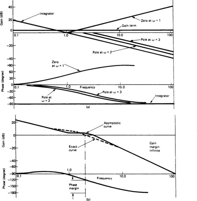
Figure 13.23 (a) Gain and phase curves for individual factors (see Figure 13.18); (b) Composite gain and phase curves. Note that the phase margin is about 60°, and the gain margin is infinite because the phase tends asymptotically to −180°
13.10.3 Nichols chart
This is a graph with the open-loop gain in decibels as co-ordinate and the phase as abscissa. The open-loop frequency response is for a particular system and is plotted with frequency ω as parameter. Now the closed-loop frequency response is given by
and corresponding lines of constant magnitude and constant phase of W(jω) are plotted on the Nichols chart as shown in Figure 13.24.
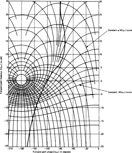
Figure 13.24 Nichols chart and plot of the system shown in Figure 13.23. Orthogonal families of curves represent constant W(jω) and constant ∠W(jω)
When the open-loop frequency response of a system has been plotted on such a chart, the closed-loop frequency response may be immediately deduced from the contours of W(jω).
13.11 State-space description
Usually in engineering, when analysing time-varying physical systems, the resulting mathematical models are in differential equation form. Indeed, the introduction of the Laplace transformation, and similar techniques, leading to the whole edifice of transfer-function-type analysis and design methods are, essentially, techniques for solving, or manipulating to advantage, differential equation models. In the state-space description of systems, which is the concern of this section, the models are left in the differential equation form, but rearranged into the form of a set of first-order simultaneous differential equations. There is nothing unique to systems analysis in doing this, since this is precisely the required form that differential equations are placed in if they are to be integrated by means of many common numerical techniques, e.g. the Runge–Kutta methods. Most of the interest in the state-space form of studying control systems stems from the 1950s, and intensive research work in this area has continued since then; however, much of it is of a highly theoretical nature. It is arguable that these methods have yet to fulfill the hopes and aspirations of the research workers who developed them. The early expectation was that they would quickly supersede classical techniques. This has been very far from true, but they do have a part to play, particularly if there are good mathematical models of the plant available and the real plant is well instrumentated.
Consider a system governed by the n th order linear constant-coefficient differential equation
where y is the dependent variable and u(t) is a time-variable forcing function.
From the governing differential equation we can write
i.e. the n th order differential equation has been transformed into n first-order equations. These can be arranged into matrix form:
which may be written in matrix notation as
where x = [x1, …., xn]T and is called the ‘state vector’, b = [0, 0, …, k]T and A is the n × n matrix pre-multiplying x on the right-hand side of Equation (13.3).
It can be shown that the eigenvalues of A are equal to the characteristic roots of the governing differential equation which are also equal to the poles of the transfer function Y(s)/U(s). Thus the time behaviour of the matrix model is essentially governed by the position of the eigenvalues of the A matrix (in the complex plane) in precisely the same manner as the poles govern the transfer function behaviour. Hence, if these eigenvalues do not lie in acceptable positions in this plane, the design process is to somehow modify the A matrix so that the corresponding eigenvalues do have acceptable positions (cf. the placement of closed-loop poles in the s plane).
Example Consider a system governed by the general second-order linear differential equation
The eigenvalues of the A matrix are given by the solution to the equation ![]() , i.e.
, i.e.
Now let u = r − k1x1 − k2x2 where r is an arbitrary, or reference, value or input, and k1 and k2 are constants. Note this is a feedback arrangement, since u has become a linear function of the state variables which, in a dynamic system, might be position and velocity. Substituting for u in equation (13.3), gives
The eigenvalues of the A matrix are given by the roots of ![]() and, by choosing suitable values for k1 and k2 (the feedback factors), the eigenvalues can be made to lie in acceptable positions in the complex plane. Note that, in this case, k1 alters the effective undamped natural frequency, and k2 alters the effective damping of the second-order system.
and, by choosing suitable values for k1 and k2 (the feedback factors), the eigenvalues can be made to lie in acceptable positions in the complex plane. Note that, in this case, k1 alters the effective undamped natural frequency, and k2 alters the effective damping of the second-order system.
If the governing differential equation has derivatives on the right-hand side, then the derivation of the first-order set involves a complication. Overcoming this is easily illustrated by an example. Suppose that
Note that care may be necessary in interpreting the x derivatives in a physical sense.
The state-space description is also a convenient way of dealing with multi-input/multi-output systems. A simple example is shown in Figure 13.25, where U1(s) and U2(s) are the inputs and Y1(s) and Y2(s) are the corresponding outputs, and so
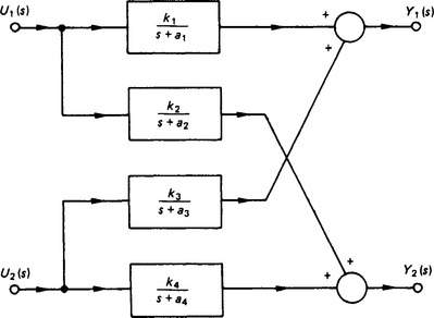
The first of these two equations may be written as
Similarly, for the second of the two equations, writing
Whence the entire set may be written as
The problem is now how to specify u1 and u2 (e.g. a linear combination of state variables similar to the simple second-order system above), so as to make the plant behave in an acceptable manner. It must be pointed out that the theory of linear matrix-differential equations is an extremely well developed mathematical topic and has been extensively plundered in the development of state-space methods. Thus a vast literature exists, and this is not confined to linear systems. Such work has, among other things, discovered a number of fundamental properties of systems (for example, controllability and observability); these are well beyond the scope of the present treatment. The treatment given here is a very short introduction to the fundamental ideas of the state-space description.
13.12 Sampled-data systems
Sampled-data systems are ones in which signals within the control-loop are sampled at one or more places. Some sort of sampling action may be inherent in the very mode of operation of some of the very components comprising the plant, e.g. thyristor systems, pulsed-radar systems and reciprocating internal combustion engines. Moreover, sampling is inevitable if a digital computer is used to implement the control laws, and/or used in condition monitoring operations. Nowadays, digital computers are routinely used in control-system operation for reasons of cheapness and versatility, e.g. they may be used not only to implement the control laws, which can be changed by software alterations alone, but also for sequencing control and interlocking in, say, the start up and safe operation of complex plant. Whatever the cause, sampling complicates the mathematical analysis and design of systems.
Normally most of the components, comprising the system to be controlled, will act in a continuous (analogue) manner, and hence their associated signals will be continuous. With the introduction of a digital computer it is necessary to digitise the signal, by an analogue-to-digital converter before the signal enters the computer. The computer processes this digital sequence, and then outputs another digital sequence which, in turn, passes to a digital-to-analogue converter. This process is shown schematically in Figure 13.26.
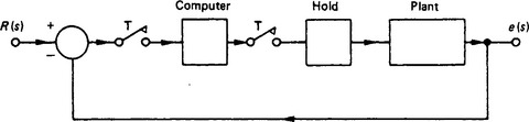
In this diagram the sampling process is represented by the periodic switch (period T), which at each sampling instant is closed for what is regarded as an infinitesimal time. The digital-to-analogue process is represented by the hold block. Thus the complete system is a hybrid one, made up of an interconnection of continuous and discrete devices. The most obvious way of representing the system mathematically is by a mixed difference-differential equation set. However, this makes a detailed analysis of the complete system difficult.
Fortunately, provided the investigator or system designer is prepared to accept knowledge of the system’s behaviour at the instants of sampling only, a comparatively simple approach having great similarity to that employed for wholly continuous systems is available. At least for early stages of the analysis or design proposal, the added complications involved in this process are fairly minor. Further, the seemingly severe restriction of knowing the system’s behaviour at the instants of sampling only is normally quite acceptable; for example, the time constants associated with the plant will generally be much longer than the periodic sampling time, so the plant effectively does not change its state significantly in the periodic time. The sampling time period is a parameter which often can be chosen by the designer, who will want sampling to be fast enough to avoid aliasing problems; however, the shorter the sampling period the less time the computer has available for other loops. Suffice it to say that the selection of the sampling period is normally an important matter.
If we take a continuous signal y(t), say, and by the periodic sampling process convert it into a sequence of values y(n), where n represents the nth sampling period, then the sequence y(n) becomes the mathematical entity we manipulate, and the values of y(t) between these samples will not be known. However, if at an early stage it is essential to know the inter-sample behaviour of the system with some accuracy, then advance techniques are available for this purpose.1 In addition, it is now fairly routine to simulate control system behaviour before implementation, and a good simulation package should be capable of illustrating the inter-sample behaviour.
We need techniques for mathematically manipulating sequences, and these are discussed in the following section.
13.13 Some necessary mathematical preliminaries
This transformation plays the equivalent role in sampled-data system studies as the Laplace transformation does in the case of continuous systems; indeed, these two transformations are mathematically related to each other. It is demonstrated below that the behaviour of sampled-data systems at the sampling instant is governed mathematically by difference equations, e.g. a linear system might be governed by the equation
where, in the case of y(n), the value of a variable at instant n is in fact dependent on a linear combination of its previous two values and the current and previous values of an independent (forcing variable) x(n). In a similar way to using the Laplace transformation to convert linear differential equations to transfer-function form, the z transformation is used to convert linear difference equations into the so-called ‘pulse transfer-function form’. The definition of the z transformation of a sequence y(n), n = 0, 1, 2, …, is
The z transformations of commonly occurring sequences are listed in Table 13.1, and a simple example will illustrate how such transformations may be found.
Suppose y(n) = nT(n = 0, 1, 2, …) such a sequence would be obtained by sampling the continuous ramp function y(t) = t, at intervals of time T. Then, by definition,
Then, applying this to the difference equation above, we have
So that, if x(n) or X(z) is given, Y(z) can be rearranged into partial fraction form, and y(n) determined from the table. For example, suppose that
Whence, from the tables we see that
The process of dividing Y(z) by z before taking partial fractions is important, as most tabulated values of the transformation have z as a factor in the numerator, and the partial function expansion process needs the order of the denominator to exceed that of the numerator.
An alternative method of approaching the z transform is to assume that the sequence to be transformed is a direct consequence of sampling a continuous signal using an impulse modulator. Thus a given signal y(t) is sampled with periodic time T, to give the assumed signal y*(t), where
where δ(t) is the delta function.
Taking the Laplace transformation of y*(t) gives the series
On making the substitution esT = z, then the resulting series is identical to that obtained by taking the z transformation of the sequence y(n). For convenience, we often write Y(z) = Z[y*(t)].
z = esT may be regarded as constituting a transformation of points in an s plane to those in a z plane, and this has exceedingly important consequences. If, for example, we map lines representing constant damping ζ, and constant natural frequency ωn, for a system represented in an s plane onto a z plane, we obtain Figure 13.27.
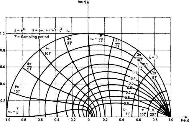
Figure 13.27 Natural frequency and damping loci in the z plane. The lower half is the mirror image of the half shown. (Reproduced from Franklin et al.,2 courtesy of Addison-Wesley)
There are important results to be noted from this diagram.
(1) The stability boundary in the s plane (i.e. the imaginary axis) transforms into the unit circle |z| = 1 in the z plane.
(2) Points in the z plane indicate responses relative to the periodic sampling time T.
(3) The negative real axis of the z plane always represents half the sampling frequency ωs, where ωs = 2π/T.
(4) Vertical lines (i.e. those with constant real parts) in the left-half plane of the s plane map into circles within the unit circle in the z plane.
(5) Horizontal lines (i.e. lines of constant frequency) in the s plane map into radial lines in the z planes.
(6) The mapping is not one-to-one; and frequencies greater than ωs/2 will coincide on the z plane with corresponding points below this frequency. Effectively this is a consequence of the Nyquist sampling theorem which states, essentially, that faithful reconstruction of a sampled signal cannot be achieved if the original continuous signal contained frequencies greater than one-half the sampling frequency.
A vitally important point to note is that all the roots of the denominator of a pulse transfer function of a system must fall within the unit circle, on the z plane, if the system is to be stable; this follows from (1) above.
13.14 Sampler and zero-order hold
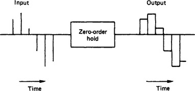
The sampler produces a series of discrete values at the sampling instant. Although in theory these samples exist for zero time, in practice they can be taken into the digital computer and processed. The output from the digital computer will be a sequence of samples with, again in theory, each sample existing for zero time. However, it is necessary to have a continuous signal constructed from this output, and this is normally done using a zero-order hold. This device has the property that, as each sample (which may be regarded as a delta function) is presented to its input, it presents the strength of the delta function at its output until the next sample arrives, and then changes its output to correspond to this latest value, and so on.
This is illustrated diagrammatically in Figure 13.28. Thus a unit delta function δ(t) arriving produces a positive unit-value step at the output at time t. At time t = T, we may regard a negative unity-value step being superimposed on the output. Since the transfer function of a system may be regarded as the Laplace transformation of the response of that system to a delta function, the zero-order hold has the transfer function
13.15 Block diagrams
In a similar way to their use in continuous-control-system studies, block diagrams are used in sampled-data-system studies. It is convenient to represent individual pulse transfer functions in individual boxes. The boxes are joined together by lines representing their z transformed input/output sequences to form the complete block diagrams. The manipulation of the block diagrams may be conducted in a similar fashion to that adopted for continuous systems. Again, it must be stressed that such manipulation breaks down if the boxes load one another.
Consider the arrangement shown in Figure 13.29. Here we have a number of continuous systems, represented by their transfer functions, in cascade. However, a sampler has been placed in each signal line, and so for each box we may write
This, of course, generalises for n similar pulse transfer functions in series to give
It is necessary to realise that this result does not apply if there is no sampler between two or more boxes. As an illustration, Figure 13.30(a) shows the arrangement for which the above result applies. We have
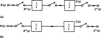
Figure 13.30 Two transfer functions with (a) sampler interconnection and (b) with continuous signal connecting transfer functions
whence (see Table 13.1)
whence (see Table 13.1)
Figure 13.30(b) shows the arrangement without a sampler between G1(s) and G2(s), and so
Note that Z[G1(s)G2(s)] is often written G1G2(z), and thus, in general, G1(z)G2(z) ≠ G1G2(z).