
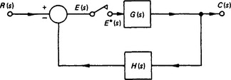
13.16 Closed-loop systems
Figure 13.31 shows the sampler in the error channel of an otherwise continuous system. We may write
If the sampler is in the feedback loop, as shown in Figure 13.32, a similar analysis would show that
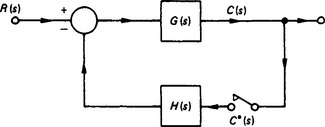
Note that, in this case, it is not possible to take the ratio C(z)/R(z). We may conclude that the position of the sampler(s) within the loop has a vitally important effect on the behaviour of the system.
Example Consider the arrangement shown in Figure 13.33. To calculate the pulse transfer function it is necessary to determine
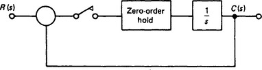
Figure 13.33 Arrangement used in the example in Section 13.16
Consider (from Table 13.1)
13.17 Stability
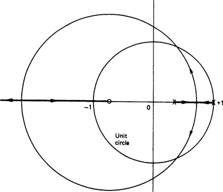
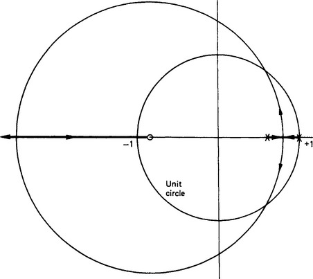
It should be appreciated from the above that, in general, C(z)/R(z) results in a ratio of polynomials in z in a similar way as, for continuous systems, C(s)/R(s) results in a ratio of polynomials in s. Thus, just as the equation 1+G(s)H(s) = 0 is called the ‘characteristic equation’ for the continuous system, 1+GH(z) = 0 is the characteristic equation for the sampled-data system. Both of these characteristic equations are polynomials in their respective variables, and the positions of the roots of these equations determine the characteristic behaviour of the corresponding closed-loop systems. Mathematically, the process of determining the roots is identical in the two cases. The difference between the two characteristic equations arises because of the need to interpret the effects of the location of the roots, when they are plotted in their respective s and z planes, on the two plants. For continuous systems, if any of these poles are located in the right-half s plane, then the system is unstable. Similarly, since the whole of the left-hand s plane maps into the unit-circle of the z plane under the transformation z = esT, then in the simple-data case, for stability all of the roots of 1+GH(z) = 0 must lie within the unit circle.
Much of the design process of control systems is to arrange for the roots of the characteristic equation to locate at desired positions in either the s or z plane. It will be recalled, from continuous theory, that the locus of these roots, as a particular parameter is varied, may be determined by using the root-locus technique. Thus, since the characteristic equation of the sample-data system has a similar form (i.e. a polynomial), the root-locus technique may be applied to 1+GH(z) = 0 in exactly the same way. Only once the root-locus has been determined is there a difference in interpreting the effects of pole positions between the two cases.
13.18 Example
Consider the system shown in Figure 13.34, and suppose that the requirement is to draw the root-locus diagrams for, say, sampling periods of 1 and 0.5 secs.
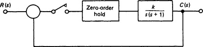
Figure 13.34 Arrangement used in the example in Section 13.18
The first requirement is to determine the pulse-transfer function for the open loop, i.e. G(z):

where, from Table 13.2, we have
Table 13.2
| Settling band | Optimum ‘b’ | Settling time |
| 20% | 0.45 | 1.80 |
| 15% | 0.55 | 2.00 |
| 10% | 0.60 | 2.30 |
| 5% | 0.70 | 2.80 |
| 2% | 0.80 | 3.50 |
Both of these equations have two real poles and one zero pole, and the root loci are as shown in Figure 13.35 and 13.36. It can be seen that the difference in the two sampling times T causes fairly dramatic changes; when T = 1 secs the system becomes unstable at K = 1.9, and when T = 0.5 secs the system becomes unstable at K = 3.9. The process of drawing the root locus for either a continuous plant or a sampled-data plant is identical. It is the interpretation of the positions of the roots that is different, although in both cases the design is to place the roots in acceptable locations in the two planes. It is possible to use Bode diagrams in sampled-data design work and this is explained in many of the references given in the Bibliography at the end of this chapter.
13.19 Dead-beat response
Consider the system shown above where T = 1 secs and K = 1; suppose that compensation of the form
is inserted immediately after the sampler. Then it is easy to show that
i.e. r(t) is a unit step function, then
i.e. c(0) = 0, c(1) = 0.582 and c(n) = 1, for n = 2, 3, ….
The implication is that c(t) has reached its target position after two sample periods. If an n th order system reaches its target position in, at most, n th sampling instants, then this is called a ‘dead-beat response’; a controller that achieves this, such as D(z) above, is called a ‘dead-beat controller’ for this system. This is an interesting response, for it is not possible to achieve this with a continuous control system.
At least two dangers are inherent in dead-beat controllers:
(1) the demanded controller outputs during the process may be excessive; and
(2) there may be an oscillation set up which is not detected without further analysis.
In fact, the system is only ‘dead beat’ at the sampling instants. Indeed, in the above example, there is an oscillation between sampling instants of about 10% of the step value. However, theoretically it is possible for a sampled-data system to complete a transient of the above nature in finite time.
13.20 Simulation
Regardless of the simulation language to be used, a necessary prerequisite is a description of the system of interest by a mathematical model. Some physical systems can be described in terms of models that are of the state transition type. If such a model exists, then given a value of the system variable of interest, e.g. voltage, charge position, displacement, etc., at time t, then the value of the variable (state) at some future time t+Δt can be predicted. The prediction of the variable of interest (state variable) x(t) at time t+Δt, given a state transition model S, can be expressed by the state equation:
Equation (13.5) shows that the future state is a function of the current state x(t) at the current time t and the time increment Δt. Thus, once the model is known, from either empirical or theoretical considerations, Equation (13.5), given an initial condition (value), allows for the recursive computation of x(t) for any number of future steps in time. For an initial value of the state variable ![]() at time t1, then
at time t1, then
then letting t2 = t1+Δt, Equation (13.5) for the next time step Δt, becomes
Obviously, this operation is continued until the calculation of the state variable has been performed for the total time period of interest.
Systems of interest will clearly not be characterised only by a single state variable but by several state variables. Figure 13.37 is a schematic representation of a multi-variable system that has r inputs, n states and m outputs.
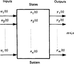
In general, the simulation will involve calculation of all of the state variables, even though the response of only a selected number of output variables is of interest. For many systems, the output variables may well exhibit a simple one-to-one correspondence to the state variables. As shown by the representation in Figure 13.37, the values of the state variables depend on the inputs to the system. For a single interval, between the k and k+1 time instants, the state equations for the n state variable system for a change in the j th input (j ≤ r)uj(t) is written as
The above system of equations, a collection of difference equations, would be used to predict the state variables x1, x2, …, xn at time intervals of Δt from the initial time t0 until the total time duration of interest T = t0+K Δt. For engineering systems, the dependent variable will generally be a continuous variable. In this case the system description will be in terms of a differential equation of the form
Recalling basic calculus for a small time increment, the left-hand side of Equation (13.7) can be expressed as
so, for a small time increment Δt, Equation (13.7) can be written as
Equation (13.8) is a form of Equation (13.5), so for a small time increment, a first-order ordinary differential equation can be approximated by a state transition representation.
It thus follows from the preceding discussion that, in digital continuous system simulation, the principal numerical task is the approximate integration of Equation (13.7). For a small time increment DT, the integration step size, the computation involves the evaluation of the difference equation
which can be written explicitly as
where DT = tk+1− tk. The calculation starts with a known value of the initial state x(0) at time t0 and proceeds successively to evaluate x(t1), x(t2), etc. The computation involves successive computation of x(tk+1) by alternating calculation of the derivative g[x(tk), tk] followed by integration to compute x(tk+1) at time tk+1 = tk+ DT.
Obviously, most physical systems will be described by second or higher order ordinary differential equations so the higher order equation must be re-expressed in terms of a group of first-order ordinary differential equations by introducing state variables. For an n th order equation,
the approach involves the introduction of new variables as state variables to yield the following first-order differential equations
It should be noted that this equation can be expressed in shorthand notation as a vector-matrix differential equation. In an analogous manner, Equation (13.6) can be expressed as a vector different equation. There is no unique approach to the selection of state variables for system representation, but for many systems the choice of state variables will be obvious. In electric circuit problems, capacitor voltages and inductor currents would be logical choices, as would position, velocity and acceleration for mechanical systems.
13.20.2 Integration schemes
The simple integration step, embodied by the first-order Euler form in Equation (13.9a) only provides a satisfactory approximation of the solution of the differential equation, within specified error limits, for a very small integration step size DT. Since the small integration interval leads to substantial computing effort and to round-off error accumulation, all digital simulation languages use improved integration schemes. Despite the wide variety of different integration schemes that are available in the many different simulation languages, the calculational approach can be categorised into two groups. The types of algorithm are:
(1) Multi-step formulae In such algorithms, the value of x(t+DT) is not calculated by the simple linear extrapolation of Equation (13.9a). Rather than use only x(t) and one derivative value, the algorithms use a polynomial approximation based on past values of x(t) and g[x(t), t], that is at times t − DT, t − 2DT, etc.
(2) Runge–Kutta formulae In Runge–Kutta type algorithms, the derivative value used for the calculation of x(t+DT) is not the point value at time t. Instead, two or more approximate derivative values in the interval t, t+DT are calculated and then a weighted average of these derivative values is used instead of a single value of the derivative to compute x(t+DT).
13.20.3 Organisation of problem input
Most simulation language input is structured into three separate sections, although in some programs the statement can be used with limited sectioning of the program. A typical structure and the type of statements, functions or parts of the simulation program that appear are as follows.
Problem documentation (e.g. name, date, etc.).
Initial conditions for state variables.
Parameter values (problem variables that may not be constant, problem time, integration order, integration step size, etc.).
Integration statements (including any control parameters not given in the initialisation section).
Conditional statements (e.g. total time, variable(s), value(s), etc.).
Output (print/plot/display) option(s).
Output format (e.g. designation of independent variable; increment for independent variable; dependent variable(s) to be output; maximum and minimum values of variable(s); or automatic scaling; total number of points for the independent variable or total length of time).
It should be understood that the specific form of the statements within each section is not exactly the same for all digital simulation languages. However, from the continuous system modelling package (CSMP) simulation programs presented in the next section, with the aid of the appropriate language manual, there should be no difficulty in formulating a simulation program using any continuous system simulation language (CSSL)-type digital simulation program.
13.20.4 Illustrative example
Simulation programs are presented, using the CSMP language, that would be suitable for investigating system dynamic behaviour. The system model, although relatively simple in nature, is typical of those used for system representation.
13.20.4.1 Example
Frequently, it will be found that system dynamic behaviour can be described by a differential equation of the form
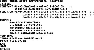
Use of CSMP for studying the dynamic behaviour of a system described by a high-order differential equation is illustrated here using a simulation program for the differential equation
Development of the simulation program follows logically by rewriting Equation (13.13) as
A block diagram showing the successive integrations to be solved for the dependent variable y is given in Figure 13.38. As can be seen from the labelling on the diagram, the output of the integration blocks is successive derivative values and the dependent variable. In fact, the output of each integration block is a state variable. This becomes obvious by introducing new variables, x1, x2, x3 defined as:
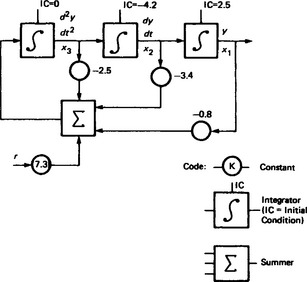
which allows Equation (13.14) to be expressed as
A program for solving equation (13.15) is given in Figure 13.39. Examination of the program shows that the value of the forcing function r is not constant but varies with time. The variation is provided using the quadratic interpolation function, NLFGEN. Total simulation time is set for 6 min with the interval for tabular output specified as 0.2 min. The time unit is determined by the problem parameters. It is to be noted that the program does not include any specification for the method of integration. The CSMP language does not require that a method of integration be given, but a particular method may be specified. If a method is not given, then by default the variable step size fourth-order Runge–Kutta method is used for calculation. The initial step size, by default, is taken as 1/16 of the PRDEL (or OUTDEL) value. Minimum step size can be limited by giving a value for DELMIN as part of the TIMER statement. If a DELMIN value is not given then, by default, the minimum step size is FINTIM × 10−7.
13.21 Multivariable control
Classical process control analysis is concerned with single loops having a single setpoint, single actuator and a single controlled variable. Unfortunately, in practice, plant variables often interact, leading to interaction between control loops. A typical interaction is shown on Figure 13.40, where a single combustion air fan feeds several burners in a multizone furnace. An increase in air flow, via V1 say to raise the temperature in zone 1, will lead to a reduction in the duct air pressure Pd, and a fall in air flow to the other zones. This will lead to a small fall in temperature in the other zones which will cause their temperature controllers to call for increased air flow which affects the duct air pressure again. The temperature control loops interact via the air valves and the duct air pressure.
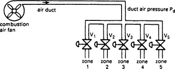
Figure 13.40 A typical example of interaction between variables in multi-variable control. The air flows interact via changes in the duct air pressure
Where interaction between variables is encountered an attempt should always be made to remove the source of the interaction, as this leads to a simpler, more robust, system. In Figure 13.40, for example, the interaction could be reduced significantly by adding a pressure control loop which maintains duct pressure by using a VF to set the speed of the combustion airfan. Often, however, the interaction is inherent and cannot by removed.
Figure 13.41 is a general representation of two interacting control loops. The blocks C1 and C2 represent the controllers comparing setpoint R with process variable V to give a controller output U. The blocks Kab represent the transfer function relating variable a to controller output b. Blocks K11 and K12 are the normal forward control path, with blocks K21 and K12 representing the interaction between the loops.
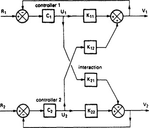
The process gain of process 1 can be defined as ΔV1/ΔU2 where Δ denotes small change. This process gain can be measured with loop 2 in open loop (i.e. U2 fixed) or loop 2 in closed loop control (i.e. V2 fixed) we can thus observe two gains
The gains will, of course vary with frequency and have magnitude and phase shift components. We can now define a relative gain λ for loop 1
If λ is unity, changing from manual to auto in loop 2 does not affect loop 1, and there is no interaction between the loops.
If λ < 1, the interaction will apparently increase process 1 gain when loop 2 is switched to automatic. If λ>1, process 1 gain will apparently be decreased when loop 2 is in automatic.
This apparent change in gain can be seen with loop 2 in manual, U2 is fixed, so K2OL is simply K11. To find K2CL we must consider what happens when loop 2 effectively shunts K11. We have
Re-arranging Equation 13.17 gives
which can be substituted in Equation 13.16 giving
The process 1 gain with loop 2 in auto is

It should be remembered that the gains Kab are dynamic functions, so λ will vary with frequency.
The term (K12K21/K11K22) is the ratio between the interaction and forward gains. This should be in the range 0 to 1. If the term is greater than unity, the interactions have more effect than the supposed process, and the process variables are being manipulated by the wrong actuators!
It is possible to determine the range of λ from the relationship (K12K21/K11K22). If this is positive, λ will be greater than unity, and loop 1 process gain will decrease when loop 2 is switched to auto. This will occur if there is an even number of Kab blocks with negative sign (0, 2 or 4). If the relationship is negative, λ will be less than unity and loop 1 process gain will increase when loop 2 is closed. This occurs if there is an odd number of blocks with negative sign (1 or 3).
The combustion air flow system of Figure 13.40 is redrawn on Figure 13.42(a). Increasing U1 obviously decreases V2, and increasing U2 similarly decreases V1. The interaction block diagram thus has the signs of Figure 13.42(b). There are two negative blocks, so λ is greater than unity.
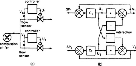
Figure 13.42 The combustion air system redrawn to show interactions: (a) block diagram; (b) interaction diagram, with two negative blocks the interaction decreases the apparent process gain and the interaction is benign
If λ is greater than unity, the interaction can be considered benign as the reduced process gain will tend to increase the loop stability (albeit at the expense of response time). The loops can be tuned individually in the knowledge that they will remain stable with all loops in automatic control.
If λ is in the range 0 < λ < 1, care must be taken as it is possible for loops to be individually stable but collectively unstable requiring a reduction in controller gains to maintain stability. The closer λ gets to zero, the greater the interaction and the more de-gaining will be required.
The calculation of dynamic interaction is difficult, even for the two variable case. With more interacting variables, the analysis becomes exceedingly complex and computer solutions are best used. Ideally, though, interactions once identified, should be removed wherever possible.
13.22 Dealing with non-linear elements
All systems are non linear to some degree. Valves have non linear transfer functions, actuators often have a limited velocity of travel and saturation is possible in every component. A controller output is limited to the range 4–20 mA, say, and a transducer has only a restricted measurement range.
One of the beneficial effects of closed loop control is the reduced effect of non linearities. The majority of non linearities are therefore simply lived with, and their effect on system performance is negligible. Occasionally, however, a non linear element can dominate a system and in these cases its effect must be studied.
Some non linear elements can be linearised with a suitable compensation circuit. Differential pressure flow meters have an output which is proportional to the square of flow. Following a non linear differential pressure flow transducer with a non linear square root extractor gives a linear flow measurement system.
Cascade control can also be used around a non linear element to linearise its performance as seen by the outer loop. Butterfly valves are notoriously non linear. They have an S shaped flow/position characteristic, suffer from backlash in the linkages and are often severely velocity limited. Enclosing a butterfly valve within a cascade flow loop, for example, will make the severely non linear flow control valve appear as a simple linear first order lag to the rest of the system.
There are two basic methods of analysing the behaviour of systems with non linear elements. It is also possible, of course, to write computer simulation programs and often this is the only practical way of analysing complex non linearities.
13.22.2 The describing function
If a non linear element is driven by a sine wave, its output will probably not be sinusoidal, but it will be periodic with the same frequency as the input, but of differing shape and possibly shifted in phase as shown on Figure 13.43. Often the shape and phase shift are related to the amplitude of the driving signal.
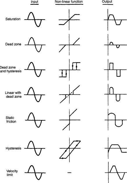
Fourier analysis is a technique that allows the frequency spectrum of any periodic waveform to be calculated. A simple pulse can be considered to be composed of an infinite number of sine waves.
The non linear output signals of Figure 13.43 could therefore be represented as a frequency spectrum, obtained from Fourier analysis. This is, however, unnecessarily complicated. Process control is generally concerned with only dominant effects, and as such it is only necessary to consider the fundamental of the spectrum. We can therefore represent a non linear function by its gain and phase shift at the fundamental frequency. This is known as the describing function, and will probably be frequency and amplitude dependant.
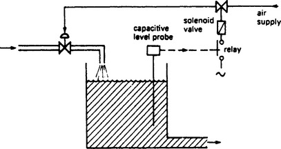
Figure 13.44 shows a very crude bang/bang servo system used to control level in a header tank. The level is sensed by a capacitive probe which energises a relay when a nominal depth of probe is submerged. The relay energises a solenoid which applies pneumatic pressure to open a flow valve. This system is represented by Figure 13.45.
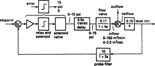
The level sensor can be considered to be a level transducer giving a 0–10 V signal over a 0.3 m range. The signal is filtered with a 2 sec time constant to overcome noise from splashing, ripples etc. The level transducer output is compared with the voltage from a setpoint control and the error signal energises or de-energises the relay. We shall assume no hysteresis for simplicity although this obviously would be desirable in a real system.
The relay drives a solenoid assumed to have a small delay in operation which applies 15 psi to an instrument air pipe to open the valve. The pneumatic signal takes a finite time to travel down the pipe, so the solenoid valve and piping are considered as a 0.5 sec transit delay. The valve actuator turns on a flow of 150 m3/min for an applied pressure of 15 psi. We shall assume it is linear for other applied pressures. The actuator/valve along with the inertia of the water in the pipe appear as a first order lag of 4 sec time constant. The tank itself appears as an integrator from flow to level.
This system is dominated by the non linear nature of the level probe and the solenoid. The rest of the system can be considered linear if we combine the level comparator, relay and solenoid into a single element which switches 0 to 15 psi according to the sign of the error signal (15 psi for negative error, i.e. low level).
This non linear element will therefore have the response of Figure 13.46. when driven with a sinusoidal error signal. The output will have a peak to peak amplitude of 15 psi regardless of the error magnitude.
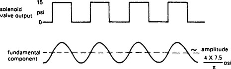
From Fourier analysis, the fundamental component of the output signal is a sine wave with amplitude 4 × 7.5/π psi as shown. The phase shift is zero at all frequencies. The non linear element of the comparator/relay/solenoid can thus be considered as an amplifier whose gain varies with the amplitude of the input signal.
For a 1 V amplitude error signal the gain is
For a 2V amplitude error signal the gain is
In general, for an E volt error signal the gain is
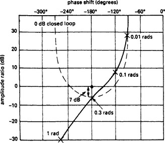
Figure 13.47 is a Nichols chart for the linear parts of the system. This has 180° phase shift for ω = 0.3 rads/sec, so if it was controlled by a proportional controller, it would oscillate at 0.3 rads/sec if the controller gain was sufficiently high. The linear system gain at this frequency is −7dB, so a proportional controller gain of 7dB would just sustain continuous oscillation.
Let us now return to our non linear level switch. This has a gain which varies inversely with error amplitude. If we are, for some reason, experiencing a large sinusoidal error signal the gain will be low. If we have a small sinusoidal error signal the gain will be high.
Intuitively we know the system of Figure 13.44 will oscillate. The non linear element will add just sufficient gain to make the Nichols chart of Figure 13.47 pass through the 0 dB/−180° origin. Self sustaining oscillations will result at 0.3 rads/sec. If these increase in amplitude for some reason, the gain will decrease causing them to decay again. If they cease, the gain will increase until oscillations recommence. The system stabilises with continuous constant amplitude oscillation.
To achieve this the non linear element must contribute 7 dB gain, or a linear gain of 2.24. From Equation 13.18 above, the gain is 9.55/E where E is the error amplitude. The required gain is thus given by an error amplitude of 9.55/2.24 = 4.26V. This corresponds to an oscillation in level of 0.426 m.
The system will thus oscillate about the set level with an amplitude of 0.4 m (the assumptions and approximations give more significant figures a relevance they do not merit) and an angular frequency of 0.4 rads/sec (period fractionally over 20 s).
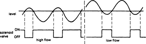
There is a hidden assumption in the above analysis that the outgoing flow is exactly half the available ingoing flow to give equal mark/space ratio at the valve. Other flow rates will give responses similar to Figure 13.48, exhibiting a form of pulse width modulation. The relatively simple analysis however has told us that our level control system will sustain constant oscillation with an amplitude of around half a metre and a period of about 20 sec at nominal flow.
Similar techniques can be applied to other non linearities; a limiter, shown on Figure 13.49(a) and (b), for example, will have unity gain for input amplitudes less than the limiting level. For increasing amplitude the apparent gain will decrease. The describing function when limiting occurs has a gain dependent on the ratio between the input signal amplitude and the limiting value as plotted on Figure 13.49(c). There is no phase shift between input and output.
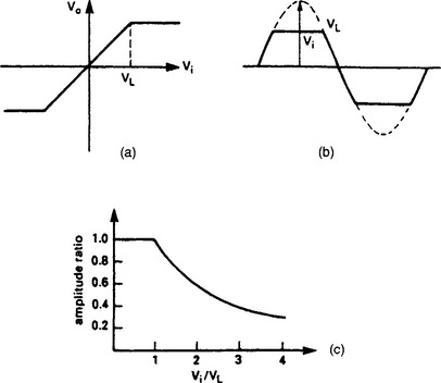
Figure 13.49 The limiter circuit: (a) relationship between input and output; (b) effect of limiting on a sine wave input signal; (c) ‘Gain’ of a limiter related to the input signal amplitude
Hysteresis, shown on Figure 13.50, introduces a phase shift, and a flat top to the output waveform. This is not the same waveform as the limiter; the top is simply levelled off at 2a below the peak where a is half the dead zone width. If the input amplitude is large compared to the dead zone, the gain is unity and the phase shift can be approximated by
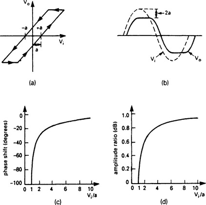
Figure 13.50 The effect of hysteresis: (a) relationship between input and output signals; (b) the effect of hysteresis on a sine wave input signal; (c) the relationship between phase shift and signal amplitude; (d) the relationship between ‘gain’ and signal amplitude
As the input amplitude decreases, the gain increases and becomes zero when the input peak to peak amplitude is less than the dead zone width. The exact relationship is complex, but is shown on Figure 13.50(c) and (d).
Non linear elements generally have gains and phase shift which increase or decrease with input amplitude (usually a representation of the error signal). Figure 13.51 illustrates the two gain cases. For a loop gain of unity, constant oscillations will result. For loop gains greater than unity, oscillations will increase in amplitude, for loop gain less than unity oscillations will decay.
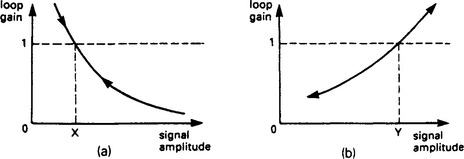
Figure 13.51 Possible relationships between gain and signal amplitude: (a) gain decreases with increasing amplitude; (b) gain increases with increasing amplitude
In Figure 13.51(a), the gain falls off with increasing amplitude. The system thus tends to approach point X as large oscillations will decay and small oscillations increase. The system will oscillate at whatever gain gives unity loop gain. This is called limit cycling. Most non linearities (bang-bang servo, saturation etc.) are of this form.
Where loop gain increases with amplitude as Figure 13.51(b), decreasing gain gives increasing damping as the amplitude decreases, so oscillations will quickly die away. This response is sometimes deliberately introduced into level controls. If, however, the system is provoked beyond Y by a disturbance, the oscillation will rapidly increase in amplitude and control will be lost.
13.22.3 State space and the phase plane
Figure 13.52(a) shows a simple position control system. The position is sensed by a potentiometer, and compared with a setpoint from potentiometer RV1. The resulting error signal is compared with an error ‘window’ by comparators C1, C2. Preset RV2 sets the deadband, i.e. the width of the window. The comparators energise relays RLF and RLR which drive the load to the forward and reverse respectively.
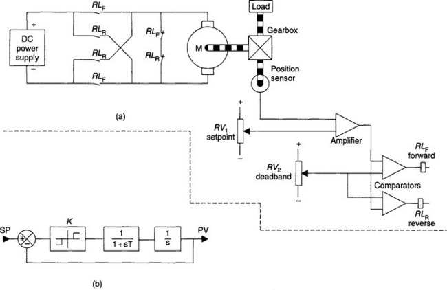
Initially, we shall analyse the system with RV2 set to zero, i.e. no deadband. This has the block diagram of Figure 13.52(b), with a first order lag of time constant T arising from the inertia of the system, and the integral action converting motor velocity to load position.
The system is thus represented by
where K represents the acceleration resulting from the motor torque and inertia with the sign of K indicating the sign of the error. This has the solution
where x0 and V0 respectively represent the initial position and velocity.
Differentiating gives the velocity, V
Equations 13.20 and 13.21 fully describe the behaviour of the system. These can be plotted graphically as Figure 13.53 with velocity plotted against position for positive K for various times from t = 0. Each curve represents a different starting condition; curve D, for example, starts at x0 = −5 and v0 = −2
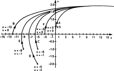
Figure 13.53 Relationship between position and velocity for positive values of K for various initial conditions
In each case, the curve ends towards v = 2 units/sec as t gets large. The family of curves have an identical shape, and the different starting conditions simply represent a horizontal shift of the curve.
A similar family of curves can be drawn for negative values of K. These are sketched on Figure 13.54. In this case, the velocity tends towards V = −2 units/sec.
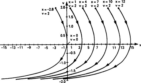
Figure 13.54 Relationship between position and velocity for negative values of K for various initial conditions
Given these curves, we can plot the response of the system. Let us assume that the system is stationary at x = −5, and the setpoint is switched to +5. The subsequent behaviour is shown on Figure 13.55. The system starts by initially following the curve passing through x = −5, V = 0 for positive K, crossing x = 0 with a velocity 1.5 units/sec, reaching the setpoint at point X with a velocity of 1.76 units/sec. It cannot stop instantly however, so it overshoots.
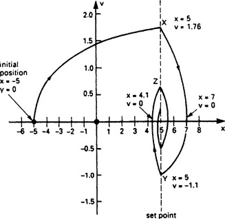
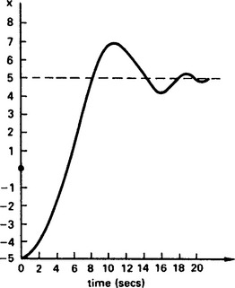
At the instant the overshoot occurs K switches sign. The system now has a velocity of +1.76, with K negative, so it follows the corresponding curve of Figure 13.54 from point X to point Y. It can be seen that an overshoot to x = 7 occurs. At point Y, another overshoot occurs and K switches back positive. The system now follows the curve to Z with an undershoot of x = 4.1. At Z another overshoot occurs and the system spirals inwards as shown. The predicted step response is shown on Figure 13.56.
In Figure 13.57(a), the deadband control (RV2 on the earlier Figure 13.52) has been adjusted to energise RLF for error voltages more negative than −1 unit and energise RLR for error voltages above +1 unit. There is thus a dead-band 2 units wide around the setpoint.
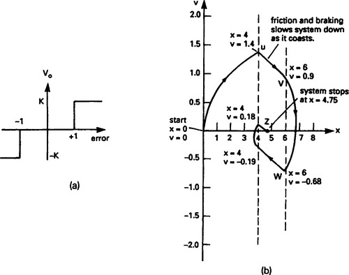
Figure 13.57 System with deadband and friction: (a) deadband response; (b) position/velocity curve for setpoint change from x = 0 to x = 5. Note system does not attain the setpoint
Figure 13.57(b) shows the effect of this deadband. We will assume initial values of x0 = 0, v0 = 0 when we switch the setpoint to x = 5. The system accelerates to point U (x = 4, v = 1.40) at which point RL1 de-energises. The system loses speed (K=0) until point V, where the position passes out of the deadband and RLR energises. The system reverses, and re-enters the deadband at point W, where RLF de-energises. An undershoot then occurs (X to Y) where the deadband is entered for the last time, coming to rest at point Z (x = 4.75, v = 0).
The position x and velocity dx/dt completely describe the system and are known as state variables. A linear system can be represented as a set of first order differential equations relating the various state variables. For a second order system there are two state variables, for higher order systems there will be more.
For the system described by Equation 13.19, we can denote the state variables by x (position) and v (velocity). For a driving function K, we can represent the system by Figure 13.58 which is called a state space model. This describes the position control system by the two first order differential equations.
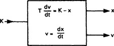
Figure 13.56 and Figure 13.57 plot velocity against position, and as such are plots relating state variables. For two state variables (from a second order system) the plot is known as a phase plane. For higher order systems, a multi-dimensional plot, called state space, is required. Plots such as Figure 13.53 and Figure 13.54 which show a family of possible curves are called phase plane portraits.
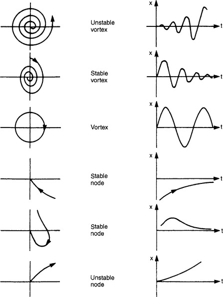
Similar phase planes can be drawn for other non linearities such as saturation, hysteresis etc. Various patterns emerge, which are summarised on Figure 13.59. The system behaviour can be deduced from the shape of the phase trajectory.
In a linear closed loop system stability is generally increased by adding derivative action. In a position control system this is equivalent to adding velocity (dx/dt) feedback. The behaviour of a non linear system can also be improved by velocity feedback. In Figure 13.60(a) velocity feedback has been added to our simple Bang/Bang position servo.
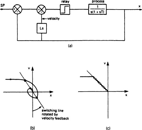
Figure 13.60 Addition of velocity feedback to a non-linear system: (a) block diagram of velocity feedback; (b) system behaviour on velocity/position curve; (c) overdamped system follows the switching line
The switching point now occurs where
This is a straight line of slope −1/L, passing through x = Sp, v = 0 on the phase plane. Note that L has the units of time. The line is called the switching line, and advances the changeover as shown on Figure 13.60(b), thereby reducing the overshoot. Too much velocity feedback as Figure 13.60(c) simulates an overdamped system as the trajectory runs to the setpoint down the switching line.
13.23 Disturbances
A closed loop control system has to deal with the malign effects of outside disturbances. A level control system, for example, has to handle varying throughput, or a gas fired furnace may have to cope with changes in gas supply pressure. Although disturbances can enter a plant at any point, it is usual to consider disturbances at two points; supply disturbances at the input to the plant and load/demand disturbances at the point of measurement as shown on Figure 13.61(a).
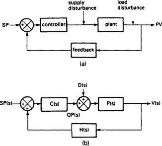
Figure 13.61 The effect of disturbances: (a) points of entry for disturbances; (b) block diagram of disturbances
The closed loop block diagram can be modified to include disturbances as shown on Figure 13.61(b). A similar block diagram could be drawn for load disturbances or disturbances entering at any point by subdividing the plant block. By normal analysis we have
Equation 13.22 has two components; the first relates the plant output to the setpoint and is the normal closed loop transfer function GH/(1+GH). The product of controller and plant transfer function C.P. is the forward gain G. The second term relates the performance of the plant to disturbance signals. In general, closed loop control reduces the effect of disturbances. If the plant was run open loop, the effect of the disturbances on the output would be simply
From Equation 13.22 with closed loop control, the effect of the disturbance is
i.e. it is reduced providing the magnitude of (1+HCP) is greater than unity. If the magnitude of (1+HCP) becomes less than unity over some range of frequencies, closed loop control will magnify the effect of disturbances in that frequency range. It is important, therefore, to have some knowledge of the frequency spectra of expected disturbances.
13.23.2 Cascade control
Closed loop control gives increased performance over open loop control, so it would seem logical to expect benefits from adding an inner control loop around plant items that are degrading overall performance. Figure 13.62 shows a typical example, here the output of the outer loop controller becomes the setpoint for the inner controller. Any problems in the inner loop (disturbances, non linearities, phase lag etc.) will be handled by the inner controller, thereby improving the overall performance of the outer loop. This arrangement is known as cascade control.
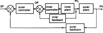
To apply cascade control, there must obviously be some intermediate variable that can be measured (Pvi on Figure 15.62) and some actuation point that can be used to control it.
Cascade control brings several benefits. The secondary controller will deal with disturbances before they can affect the outer loop. Phase shift within the inner loop is reduced, leading to increased stability and speed of response in the outer loop. Devices with inherent integral action (such as a motorised valve) introduce an inherent −90° integrator phase lag. This can be removed by adding a valve positioner in cascade. Cascade control will also reduce the effect of non linearities (e.g. non linear gain, backlash etc.) in the inner loop.
There are a few precautions that need to be taken, however. The analysis so far ignores the fact that components saturate and stability problems can arise when the inner loop saturates. This can be overcome by limiting the demands that the outer loop controller can place on the inner loop (i.e. ensuring the outer loop controller saturates first) or by providing a signal from the inner to the outer controller which inhibits the outer integral term when the inner loop is saturated.
The application of cascade control requires an intermediate variable and control action point, and should include, if possible, the plant item with the shortest time constant. In general, high gain proportional only control will often suffice for the inner loop, any offset is of little concern as it will be removed by the outer controller. For stability, the inner loop must always be faster than the outer loop.
Tuning a system with cascade control requires a methodical approach. The inner loop must be tuned first with the outer loop steady in manual control. Once the inner loop is tuned satisfactorily, the outer loop can be tuned as normal. A cascade system, once tuned, should be observed to ensure that the inner loop does not saturate, which can lead to instability or excessive overshoot on the outer loop. If saturation is observed, limits must be placed on the output of the outer loop controller, or a signal provided to prevent integral windup as described later in Section 13.27.6
13.23.3 Feedforward
Cascade control can reduce the effect of disturbances occurring early in the forward loop, but generally cannot deal with load/demand disturbances which occur close to, or affect directly the process variable as there is no intermediate variable or accessible control point.
Disturbances directly affecting the process variable must produce an error before the controller can react. Inevitably, therefore, the output signal will suffer, with the speed of recovery being determined by the loop response. Plants which are difficult to control tend to have low gains and long integral times for stability, and hence have a slow response. Such plants are prone to error from disturbances.
In general a closed loop system can be considered to behave as a second order system, with a natural frequency ωn, and a damping factor. At frequencies above ωn, the closed loop gain falls off rapidly (at 12 dB/octave). Disturbances occurring at a frequency much above 2ωn will be uncorrected. If the closed loop damping factor is less the unity (representing an underdamped system), the effect of disturbances with frequency components around ωn can be magnified.
Figure 13.63(a) shows a system being affected by a disturbance. Cascade control cannot be applied because there is no intermediate variable between the point of entry and the process variable. If the disturbance can be measured, and its effect known, (even approximately), a correcting signal can be added to the controller output signal to compensate for the disturbance as shown on Figure 13.63(b). This is known as feedforward control.
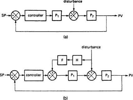
Figure 13.63 Effect of a disturbance reduced by feedforward: (a) a system to which cascade control cannot be applied being subject to a disturbance; (b) correcting signal derived by measuring the disturbance
This correcting signal, arriving by blocks H, F, and P1 should ideally exactly cancel the original disturbance, both in the steady state and dynamically under changing conditions. The transfer functions of the transducer H and plant P1 are fixed, with F a compensator block designed to match H and P1.
In general, the compensator block transfer function will be
If the plant acts as a simple lag with time constant T (i.e. 1/(1+s T)), the compensator will be a simple lead (1+s T). In many cases a general purpose compensator (1+s Ta)/(1+s Tb) is used.
The feedforward compensation does not have to match exactly the plant characteristics; even a rough model will give a significant improvement (although a perfect model will give perfect control). In most cases a simple compensator will suffice.
Cascade control can usually deal with supply disturbances and feedforward with load or demand disturbances. These neatly complement each other so it is very common to find a system where feedforward modifies the setpoint for the inner cascade loop.
13.24 Ratio control
It is a common requirement for two flows to be kept in precise ratio to each other; gas/oil and air in combustion control, or reagants being fed to a chemical reactor are typical examples.
13.24.2 Slave follow master
In simple ratio control, one flow is declared to be the master. This flow is set to meet higher level requirements such as plant throughput or furnace temperature. The second flow is a slave and is manipulated to maintain the set flow ratio.
The controlled variable here is ratio, not flow, so an intuitive solution might look similar to Figure 13.64 where the actual ratio A/B is calculated by a divider module and used as the process variable for a controller which manipulated the slave control valve.
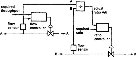
Figure 13.64 An intuitive, but incorrect, method of ratio control. The loop gain varies with throughput
This scheme has a hidden problem. The slave loop includes the divider module and hence the term A. The loop gain varies directly with the flow A, leading to a sluggish response at low flows and possible instability at high flow. If the inverse ratio B/A is used as the controller variable the saturation becomes worse as the term 1/A now appears in the slave loop giving a loop gain which varies inversely with A, becoming very high at low flows. Any system based on Figure 13.64 would be impossible to tune for anything other than constant flow rates.
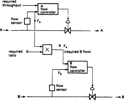
Ratio control systems are often based on Figure 13.65. The master flow is multiplied by the ratio to produce the setpoint for the slave flow controller. The slave flow thus follows the master flow. Note that in the event of failure in the master loop (a jammed valve for example) the slave controller will still maintain the correct ratio.
The slave flow will tend to lag behind the master flow. On a gas/air burner, the air flow could be master and the gas loop the slave. Such a system would run lean on increasing heat and run rich on decreasing heat. To some extent this can be overcome by making the master loop slower acting than the slave loop, possibly by tuning.
In a ratio system, a choice has to be made for master and slave loops. The first consideration is usually safety. In a gas/air burner, for example, air master/gas slave (called gas follow air) is usually chosen as most failures in the air loop cause the gas to shut down. If there are no safety considerations, the slowest loop should be the master and the fastest loop the slave to overcome the lag described above. Since ‘fuel’ (in both combustion and chemical terms) is usually the smallest flow in a ratio system and consequently has smaller valves/actuators, the safety and speed requirement are often the same.
The ratio block is a simple multiplier. If the ratio is simply set by an operator this can be a simple potentiometer acting as a voltage divider (for ratios less the unity) or an amplifier with variable gain (for ratios greater than unity). In digital control systems, of course, it is a simple multiply instruction. If the ratio is to be changed remotely (a trim control from an automatic sampler on a chemical blending system for example) a single quadrant analog multiplier is required.
Ratio blocks are generally easier to deal with in digital systems working in real engineering units. True ratios (an air/gas ratio of 10/1 for example) can then be used. In analog systems the range of the flow meters needs to be considered. Suppose we have a master flow with FSD of 120001/min, a slave flow of FSD 20001/min and a required ratio (master/slave) of 10/1. The required setting of R on Figure 13.65 would be 0.6. In a well designed plant with correctly sized pipes, control valves and flow meters, analog ratios are usually close to unity. If not, the plant design should be examined.
Problems can arise with ratio systems if the slave loop saturates before the master. A typical scenario on a gas follow air burner control could go; the temperature loop calls for a large increase in heat (because of some outside influence). The air valve (master) opens fully, and the gas valve follows correctly but cannot match the requested flow. The resulting flame is lean and cold (flame temperature falls off rapidly with too lean a ratio) and the temperature does not rise. The system is now locked with the temperature loop demanding more heat and the air/gas loops saturated, delivering full flow but no temperature rise. The moral is; the master loop must saturate before the slave. If this is not achieved by pipe sizing the output of the master controller should be limited.
13.24.3 Lead lag control
Slave follow Master is simple, but one side effect is that the mixture runs lean for increasing throughput and rich for decreasing throughput because the master flow must always change first before the slave can follow. There is also a possible safety implication because a failure of the slave valve or controller could lead to a gross error in the actual ratio such as the fuel valve wide open and the air valve closed.
Better performance can be obtained with a system called Lead-lag control shown for an air/fuel burner on Figure 13.66. This uses cross linking and selectors to provide an air setpoint which is the highest of the external power demand signal or ratio’d fuel flow. The fuel setpoint is the lowest of the external power demand or ratio’d air flow.
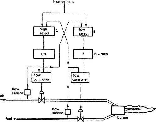
This cross linking provides better ratio during changes, both air and fuel will change together. There is also higher security; a jammed open fuel valve will cause the air valve to open to maintain the correct ratio and prevent an explosive atmosphere of unburned fuel forming.
13.25 Transit delays
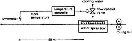
Transit delays are a function of speed, time and distance. A typical example from the steel industry is the tempering process of Figure 13.67 where red hot rolled steel travelling at 15 m/sec is quenched by passing beneath high pressure water sprays. The recovery temperature, some 50 m downstream, is the controlled variable which is measured by a pyrometer and used to adjust the water flow control valve. There is an obvious transit delay of 50/15 = 3.3 sec in the loop. A transit delay is a simple time shift which is independent of frequency.
Transit delays give an increasing phase shift with rising frequency which is de-stabilising. If conventional controllers are used significant detuning (low gain, large Ti) is necessary to maintain stability. The effect is shown on the Nichols charts of Figure 13.68 for a simple system of two first order lags controlled by a PI controller. The de-stabilising effect of the increasing phase shift can clearly be seen. Derivative action, normally a stabilising influence, can also adversely affect a loop in which a transit delay is the dominant feature.
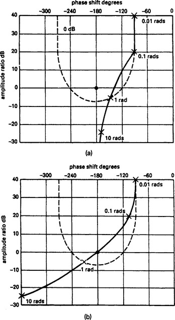
Figure 13.68 The effect of a transit delay on stability: (a) sketch of a Nichols chart for a system comprising a PI controller (K = 5, Ti − 5 s) and two first order lags of time constants 5 secs and 2 secs. The system is unconditionally stable; (b) the same system with a one second transit delay. The transit delay introduces a phase shift which increases with rising frequency and makes the system unstable
13.25.2 The Smith predictor
The effects of a transit delay can be reduced by the arrangement of Figure 13.69 called a Smith predictor. The plant is considered to be an ideal plant followed by a transit delay. (This may not be true, but the position of the transit delay, before or after the plant, makes no difference to the plant behaviour.) The plant and its associated delay are modelled as accurately as possible in the controller.
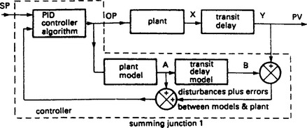
The controller output, OP, is applied to the plant and to the internal controller model. Signal A should thus be the same as the notional (and unmeasurable) plant signal X, and the signal B should be the same as the measurable controlled variable signal Y.
The PID controller however, is primarily controlling the model, not the plant, via summing junction 1. There are no delays in this loop, so the controller can be tuned for tight operation. With the model being the only loop, however, the plant is being operated in open loop control, and compensation will not be applied for model inaccuracies or outside disturbances.
Signal Y and B are therefore compared by a subtractor to give an error signal which encompasses errors from both disturbances and the model. These are added to the signal A from the plant model to give the feedback signal to the PID control block.
Discrepancies between the plant model and the real plant will be compensated for in the outer loop, so exact modelling is not necessary. The poorer the model, however, the less tight the control that can be applied in the PID block as the errors have to be compensated via the plant transit delay.
Smith predictors are usually implemented digitally, analog transit delays being difficult to construct. A digital delay line is simply a shift register in which values are shifted one place at each sample.
The Smith predictor is not a panacea for transit delays; it still takes the delay time from a setpoint change to a change in the process variable, and it still takes the delay time for a disturbance to be noted and corrected. The response to change, however, is considerably improved.
Systems with transit delays can benefit greatly from feedforward described previously in Section 13.23.3. Feedforward used in conjunction with a Smith predictor can be a very effective way of handling control systems with significant transit delays.
13.26 Stability
At first sight it would appear that perfect control can be obtained by utilising a large proportional gain, short integral time and long derivative time. The system will then respond quickly to disturbances, alterations in load and set point changes.
Unfortunately life is not that simple, and in any real life system there are limits to the settings of gain Ti and Td beyond which uncontrolled oscillations will occur. Like many engineering systems, the setting of the controller is a compromise between conflicting requirements.
13.26.2 Definitions and performance criteria
It is often convenient, (and not too inaccurate), to consider that a closed loop system behaves as a second order system, with a natural frequency ωn and a damping factor β.
It is then possible to identify five possible performance conditions, shown for a set point change and a disturbance in Figure 13.70(a) and (b).
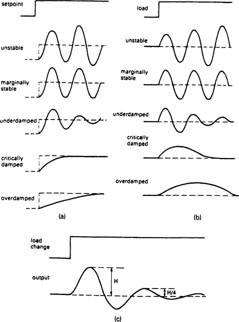
Figure 13.70 Various forms of system response: (a) step change in setpoint; (b) step change in load; (c) quarter amplitude damping
An unstable system exhibits oscillations of increasing amplitude. A marginally stable system will exhibit constant amplitude oscillations. An underdamped system will be somewhat oscillatory, but the amplitude of the oscillations decreases with time and the system is stable. (It is important to appreciate that oscillatory does not necessarily imply instability). The rate of decay is determined by the damping factor. An often used performance criteria is the ‘quarter amplitude damping’ of Figure 13.70(c) which is an underdamped response with each cycle peak one quarter of the amplitude of the previous. For many applications this is an adequate, and easily achievable response.
An overdamped system exhibits no overshoot and a sluggish response. A critical system marks the boundary between underdamping and overdamping and defines the fastest response achievable without overshoot.
For a simple system the responses of Figure 13.70(a) and (b) can be related to the gain setting of a P only controller, overdamped corresponding to low gain with increasing gain causing the response to become underdamped and eventually unstable.
It is impossible for any system to respond instantly to disturbances and changes in set point. Before the adequacy of a control system can be assessed, a set of performance criteria is usually laid down by production staff. Those defined in Figure 13.71 are commonly used.
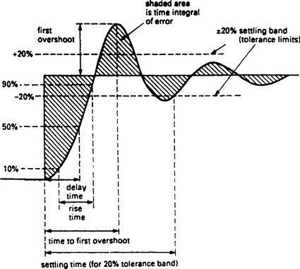
The ‘rise time’ is the time taken for the output to go from 10% to 90% of its final value, and is a measure of the speed of response of the system. The time to achieve 50% of the final value is called the ‘delay time’. This is a function of, but not the same as, any transit delays in the system. The first overshoot is usually defined as a percentage of the corresponding set point change, and is indicative of the damping factor achieved by the controller.
As the time taken for the system to settle completely after a change in set point is theoretically infinite, a ‘settling band’, ‘tolerance limit’ or ‘maximum error’ is usually defined. The settling time is the time taken for the system to enter, and remain within, the tolerance limit. Surprisingly an underdamped system may have a better settling time than a critically damped system if the first overshoot is just within the settling band. Table 13.2 shows optimum damping factors for various settling bands. The settling time is defined in units of 1/ωn.
The shaded area is the integral of the error and this can also be used as an index of performance. Note that for a system with a standing offset (as occurs with a P only controller) the area under the curve will increase with time and not converge to a final value. Stable systems with integral action control have error areas that converge to a finite value. The area between the curve and the set point is called the integrated absolute error (IAE) and is an accepted performance criterion.
An alternative criterion is the integral of the square of the instantaneous error. This weights large errors more than small errors, and is called integrated squared error (ISE). It is used for systems where large errors are detrimental, but small errors can be tolerated.
The performance criteria above were developed for a set point change. Similar criteria can be developed for disturbances and load changes.
13.26.3 Methods of stability analysis
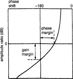
The critical points for stability are open loop unity gain and a phase shift of −180°. It is therefore reasonable to give two figures of ‘merit’:
(a) The Gain Margin is the amount by which the open loop gain can be increased at the frequency at which the phase shift is −180°. It is simply the inverse of the gain at this critical frequency, for example if the gain at the critical frequency is 0.5, the gain margin is two.
(b) The Phase Margin is the additional phase shift that can be tolerated when the open loop gain is unity. With −140° phase shift at unity gain, there is a phase margin of 40°.
For a reasonable, slightly underdamped, closed loop response the gain margin should be of the order of 6–12 dB and the phase margin of the order of 40–65°.
Any closed loop control system can be represented by Figure 13.72 where G is the combined block transfer function of the controller and plant and H the transfer function of the transducer and feed back components. The output will be given by:
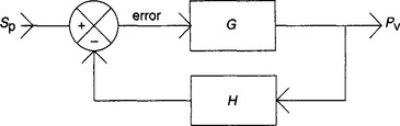
The system will be unstable if the denominator goes to zero or reverses in sign, i.e. GH < = −1. This is not as simple a relationship as might be first thought, as we are dealing with the dynamics of the process. The response of the system (gain and phase shift) will vary with frequency; generally the gain will fall and the phase shift will rise with increasing frequency. A phase shift of 180° corresponds to multiplying a sine wave by − 1, so if at some frequency the phase shift is 180° and the gain at that frequency is greater than unity the system will be unstable.
There are several methods of representing the gain/phase shift relationship, and inferring stability from the plot. Figure 13.73 is called a Bode diagram and plots the gain (in dB) and phase shift on separate graphs. Log-Lin graph paper (e.g. Chartwell 5542) is required. For stability, the gain curve must cross the 0 dB axis before the phase shift curve crosses the 180° line. From these two values, the gain margin and the phase margin can be read as shown.
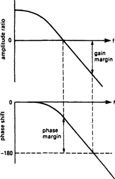
Figure 13.74 is a Nichols chart and plots phase shift against gain (in dB). For stability, the 0 dB/ −180° intersection must be to the right of the curve for increasing frequency. Nichols charts are plotted on pre-printed graph paper (Chartwell 7514 for example) which allows the closed loop response to be read directly. If for example the curve is inside the closed loop 0 dB line damped oscillations will result. The gain and phase margins can again be read from the graph.
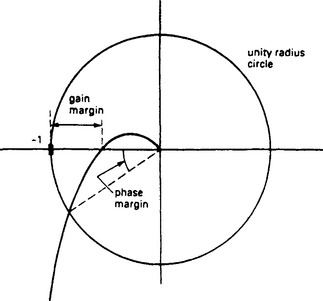
The final method is the Nyquist diagram of Figure 13.75. This plots gain again phase shift as a polar diagram (gain represented by distance from the origin). Chartwell graph paper 4001 is suitable. For stability the −180° point must be to the left of the graph for increasing frequency. Gain and phase margin can again be read from the graph.
13.27 Industrial controllers
The commercial three term controller is the workhorse of process control and has evolved to an instrument of great versatility. This section describes some of the features of practical modern microprocessor based controllers.
13.27.2 A commercial controller
The description in this section is based on the 6360 controller manufactured by Eurotherm Process Automation Ltd of Worthing, Sussex.
The controller front panel is the ‘interface’ with the operator who may have little or no knowledge of process control. The front panel controls should therefore be simple to comprehend. Figure 13.76 shows a typical layout.

The operator can select one of three operating modes—manual, automatic or remote—via the three push buttons labelled M, A, R. Indicators in each push-button show the current operating mode.
In manual mode, the operator has full control over the driven plant actuator. The actuator drive signal can be ramped up or down by holding in the M button and pressing the ![]() or
or ![]() buttons. The actuator position is shown digitally on the digital display, whilst the M button is depressed and continuously in analog form on the horizontal bargraph.
buttons. The actuator position is shown digitally on the digital display, whilst the M button is depressed and continuously in analog form on the horizontal bargraph.
In automatic mode the unit behaves as a three term controller with a set point loaded by the operator. The unit is scaled into engineering units (i.e. real units such as °C, psi, litres/min) as part of the set up procedure so that the operator is working with real plant variables. The digital display shows the set point value when the SP button is depressed and the value can be changed with the ![]() and
and ![]() buttons.
buttons.
The set point is also displayed in bargraph form on the right-hand side of the dual vertical bargraph.
Remote mode is similar to automatic mode except the set point is derived from an external signal. This mode is used for ratio or cascade loops (see Sections 13.23 and 13.24) and batch systems where the setpoint has to follow a predetermined pattern. As before the setpoint is displayed in bargraph form and the operator can view, but not change, the digital value by depressing the SP button.
The process variable itself is displayed digitally when no push button is depressed, and continually on the left-hand bargraph. In automatic or remote modes the height of the two left-hand bargraphs should be equal, a very useful quick visual check that all is under control.
Alarm limits, (defined during the controller set up), can be applied to the process variable or the error signal. If either move outside acceptable limits, the process variable bargraph flashes, and a digital output from the controller is given for use by an external annunciator audible alarm of data logger.
Figure 13.77 shows a simple block diagram representation of a controller.
Input analog signals enter at the left-hand side. Common industrial signal standards are 0–10 V, 1–5 V, 0–20 mA and 4–20 mA. These can be accommodated by two switchable ranges 0–10 V and 1–5V plus suitable burden resistors for the current signals (a 250 ohm resistor, for example, converts 4–20 mA to 1–5 V).
4–20 mA and 0–20 mA signals used on two wire loops require a DC power supply somewhere in the loop. A floating 30 V power supply is provided for this purpose.
Open circuit detection is provided on the main PV input. This is essentially a pull up to a high voltage via a high value resistor. A comparator signals an open circuit input when the voltage rises. Short circuit detection can also be applied on the 1–5 V input (the input voltage falling below 1 V). Open circuit or short circuit PV is usually required to bring up an alarm and trip the controller to manual, with the output signal driven high, held at last value, or driven low according to the nature of the plant being controlled. The open circuit trip mode is determined by switches as part of the set up procedure.
The PV and remote SP inputs are scaled to engineering units and linearised. Common linearisation routines are thermocouples, platinum resistance thermometers and square root (for flow transducers). A simple adjustable first order filter can also be applied to remove process or signal noise. The set point for the PID algorithm is selected from the internal set point or the remote set point by the from panel auto and remote push button contacts A, R.
The error signal is obtained by a subtractor (PV and Sp both being to the same scale as a result of the scaling and engineering unit blocks). At this stage two alarm functions are applied. An absolute input alarm provides adjustable high and low alarm limits on the scaled and linearised Pv signals, and a deviation alarm (with adjustable limits) applied to the error signal. These alarm signals are brought out of the controller as digital outputs.
The basic PID algorithm is implemented digitally and includes a few variations to deal with some special circumstances. These modifications utilise the additional signals to the PID block (PV, hold, track, output balance) and are described later.
The PID algorithm output is the actuator drive signal scaled 0–100%. The PID algorithm assumes that an increasing drive signal causes an increase in PV. Some actuators, however, are reverse acting, with an increasing drive signal reducing PV. A typical example is cooling water valves which are designed to fail open delivering full flow on loss of signal. Before the PID algorithm can be used with reverse acting actuators (or reverse acting transducers) its output signal must be reversed. A set up switch selects normal or inverted PID output. Note that reverse action does not alter the polarity of the controller output, merely the sign of the gain.
The output signal is selected from the manual raise/lower signal or the PID signal by the front panel manual/auto/remote pushbuttons M, A, R. At this stage limits are applied to the selected output drive. This limiting can be used to constrain actuators to a safe working range. The output limit allows the controller output to be limited just before the actuator’s ends of travel, keeping the PV under control at all times.
Two controller outputs are provided, 0–10 V and 4–20 mA for use with voltage and current driven actuators. The linearised PV signal is also retransmitted as a 0–10 V signal for use with the separate external indicators and recorders.
13.27.3 Bumpless transfer
The output from the PID algorithm is a function of time and the values of the set point and the process variable. When the controller is operating in manual mode it is highly unlikely that the output of the PID block will be the same as the demanded manual output. In particular the integral term will probably cause the output from the PID block to eventually saturate at 0% or 100% output.
If no precautions are taken, therefore, switching from auto to manual, then back to auto again some time later will result in a large step change in controller output at the transition from manual to automatic operation.
To avoid this ‘bump’ in the plant operation, the controller output is fed back to the PID block, and used to maintain a PID output equal to the actual manual output. This balance is generally achieved by adjusting the contribution from the integral term.
Mode switching can now take place between automatic and manual modes without a step change in controller output. This is known as manual/auto balancing, preload or (more aptly) bumpless transfer.
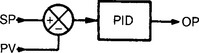
A similar effect can occur on set point changes. With a straightforward PID algorithm, a setpoint change of ΔSp will produce an immediate change in controller output of K · ΔSP where K is the controller gain. In some applications this step change in output is unacceptable. In Figure 13.78 a term K · SP is subtracted from the PID block output. The controller now responds to errors caused by changes in Pv in the normal way, but only reacts to changes in SP via the integral and derivative terms. Changes in SP thus result in a slow change in controller output. This is known as setpoint change balance, and is a switch selectable set up option.
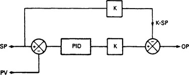
Figure 13.78 Set point change balance, the controller only follows set point changes on the integral term giving a ramped response to a change of set point
This balance signal fed back from the output to the PID block is also used when the controller output is forced to follow an external signal. This is called track mode.
As before, the PID algorithm needs to be balanced to avoid a bump when transferring between track mode and automatic mode. The feedback output signal achieves this balance as described previously.
13.27.4 Integral windup and desaturation
Large changes in SP or large disturbances to PV can lead to saturation of the controller output or a plant actuator. Under these conditions the integral term in the PID algorithm can cause problems.
Figure 13.79 shows the probable response of a system with unrestricted integral action. At time A a step change in set point occurs. The output OP rises first in a step (K × set point change) then rises at a rate determined by the integral time. At time B the controller saturates at 100% output, but the integral term keeps on rising.
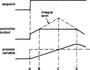
At the time C PV reaches, and passes, the required value, and as the error changes sign the integral term starts to decrease, but it takes until time D before the controller desaturates. Between times B and D the plant is uncontrolled, leading to an unnecessary overshoot and possibly even instability.
This effect is called ‘integral windup’ and is easily avoided by disabling the integral term once the controller saturates either positive or negative. This is naturally a feature of all commercial controllers, but process control engineers should always by suspicious of ‘home brew’ control algorithms constructed (or written in software) by persons without control experience.
In any commercial controller, the integral term would be disabled at point B on Figure 13.80 to prevent integral windup. The obvious question now is at what point it is re-enabled again. Point C is obviously far too late (although much better than point D in the unprotected controller).
A common solution is to desaturate the integral term at the point where the rate of increase of the integral action equals the rate of decrease of the proportional and derivative terms. This occurs when the slope of the PID output is zero, i.e. when
with e being the error and Ti and Td the controller constants.
Equation 13.23 brings the controller out of saturation at the earliest possible moment, but this can, in some cases, be too soon leading to an unnecessarily damped response. Some controllers allow adjustment of the desaturation point by adding an error limit circuit to delay the balance point to Equation 13.23 forcing the controller to remain in saturation for a longer time. The speed of desaturation and the degree of overshoot can thus be adjusted by the commissioning engineer.
13.27.5 Selectable derivative action
The term Td (de/dt) in the three term controller algorithm can be rearranged as
where SP is the set point and PV the process variable. The derivative term thus responds to changes in both the set point and the plant feedback signal.
This is not always desirable; in particular a step change in set point leads to an infinite spike controller output and a vicious ‘kick’ to the actuator. Commercial controller therefore include a selectable option for the derivative term to be based on true error (SP−PV) or purely on the value of Pv alone.
There is generally no noticeable difference in plant performance between these options; stability or the ability to deal with disturbances or load changes are unaffected, and derivative on Pv is normally the preferred choice. The only occasion when true derivative on error is advantageous is where the Pv is required to track a continually changing SP.
13.27.6 Variations on the PID algorithm
The theoretical PID algorithm is described by the equation
where e is the error, K is the gain, Ti is the integral time and Td the derivative time. Unfortunately different manufacturers use different terminology and even different algorithms.
Many manufacturers define the gain as the proportional band, denoted as PB or PB. This is the inverse of the gain expressed as a percentage, i.e
A gain of two is thus the same as a proportional band of 50%, and decreasing the proportional band increases the gain.
The integral time is commonly expressed as ‘Repeats per Minute’ or rpm. The relationship is given by:
The derivative time is often called the rate or pre-act term but these are all identical to Td.
More surprisingly there are variations on the basic algorithm. Some manufacturers use a so called ‘non interacting’ or ‘parallel’ equation which can be expressed as:
In these the three terms are totally independent. In the second version Ki is called the integral gain and Kd the derivative gain. Note that increasing Ki has the same effect as decreasing Ti. It is tempting to think that the non interacting equations are simpler to use, but in practice the theoretical model is more intuitive. In particular, as the gain K is reduced in the non interacting equation, any integral action has more effect and contributes more phase shift. Increasing or decreasing the gain with a non interacting controller can thus cause instability.
There is yet a third form of PID algorithm known as the ‘series’ equation. This can be expressed as:
This algorithm is based on pneumatic and early electronic controllers, and some manufacturers have maintained it to give backward compatibility. This has the odd characteristic that the Ti and Td controls interact with each other, with the maximum derivative action occurring when Td and Ti are set equal. In addition the ratio between Ti and Td interacts with the overall gain.
There are further variations on the way the derivative contribution is handled. We have already discussed the effect of derivative on process variable and derivative on error. Because the pure derivative term gives increasing gain with increasing frequency it amplifies any high frequency noise resulting in continual twitchy movements of the plant actuators. Many manufacturers therefore deliberately roll off the high frequency gain, either by filtering the signal applied to the derivative function or directly limiting the derivative action.
13.27.7 Incremental controllers
Diaphragm operated actuators can be arranged to fail open or shut by reversing the relative positions of the drive pressure and return spring. In some applications a valve will be required to hold its last position in the event of failure. One way to achieve this is with a motorised actuator, where a motor drives the valve via a screw thread.
Such an actuator inherently holds its last position but the position is now the integral of the controller output. An integrator introduces 90° phase lag and gain which falls off with increasing frequency. A motorised valve is therefore a destabilising influence when used with conventional controllers.
Incremental controllers are designed for use with motorised valves and similar integrating devices. They have the control algorithm
which is the time derivative of the normal control algorithm.
Incremental controllers are sometimes called boundless controllers or velocity controllers because the controller output specifies the actuator rate of change (i.e. velocity) rather than actual position.
Incremental controllers cannot suffer from integral windup per se, but it is often undesirable to keep driving a motorised valve once the end of travel is reached. End of travel limits are often incorporated in motorised valves to prevent jamming. The controller also has no real ‘idea’ of the valve true position, and hence cannot give valve position indication. If end of travel signals are available, a valve model can be incorporated into the controller to integrate the controller output to give a notional valve position. This model would be corrected whenever an end of travel limit is reached. Alternatively a position measuring device can be fitted to the valve for remote indication.
Pulse width modulated controllers are a variation on the incremental theme. Split phase motor drive valves require logic raise/lower signals, and normal proportional control can be simulated by using time proportional raise/lower outputs.
13.27.8 Scheduling controllers
Many loops have properties which change under the influence of some measurable outside variable. The gain of a flow control valve, (i.e. the change in flow for change in valve position) varies considerably over the stroke of a valve. The levitation effect of steam bubbles in a boiler drum causes the drum level control to have different characteristics under start-up, low load and high load conditions.
A scheduling controller has a built-in look up table of control parameters (gain, filtering, integral time etc.) and the appropriate values selected for the measured plant conditions.
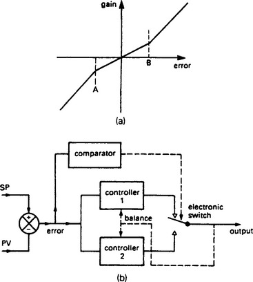
13.27.9 Variable gain controllers
Process variable noise occurs in many loops; level and flow being possibly the worst offenders. This noise causes unnecessary actuator movement, leading to premature wear and inducing real changes in the plant state. Noise can, of course, be removed by first or second order filters, but these reduce the speed of the loop and the additional phase shift from the filters can often act to de-stabilise a loop.
A controller with gain K will pass a noise signal K · n(t) to the actuator where n(t) is the noise signal. One obvious way to reduce the effect of the noise is to reduce the controller gain, but this degrades the loop performance. Usually the noise signal has a small amplitude compared with the signal range, if it has not the process will be practically uncontrollable. What is intuitively required is a low gain when the error is low, but a high gain when the error is high.
Figure 13.80(a) shows how such a scheme operates. The noise amplitude lies in the range AB, so this is made a low gain region. Outside this band the gain is much higher. The gain in the region AB should be low, but not zero, to keep the process variable at the set point. With a pure deadband (i.e. zero gain in region AB) the process variable would cycle between one side of the centre band and the other.
Figure 13.80(b) shows a possible implementation. A comparator switches between a low gain and high gain controller according to the magnitude of the error. Note that integral balancing is required between the two controllers to stop integral windup in the unselected controller.
Figure 13.80 has two gain regions. It is possible to construct a controller whose gain varies continuously with error. Such a controller has a response
where f(e) is a function of error.
where e is expressed as a percentage (0–100%) and m is a user set linearity adjustment (0 < m < 1). The abs operation (which always returns a positive sign) is necessary to prevent the controller action changing sign on negative error.
With m = 1, f(e) = 1 and Equation 13.24 behaves as a normal three term controller. With m = 0. the proportional part of Equation 13.24 follows a square law. Like Figure 13.80(a), this has low gain or small error (zero gain at zero error) but progressively increasing gain as the error increases.
Position control systems often need a fast response but cannot tolerate an overshoot. These often use Equation 13.24 with m at a low value approximating to the quadratic curve. This gives a high take off speed, but a low speed of approach.
13.27.10 Inverse plant model
The ideal control strategy, in theory, is one which mimics the plan behaviour. Given a totally accurate model of the plant, it should be possible to calculate what controller output is required to follow set point change, or compensate for a disturbance. The problem here is, of course, having an accurate plant model, but even a rough approximation should suffice as the controller output will converge to the correct value eventually.
One possible solution is shown in Figure 13.81. The process is represented by a block with transfer function K · f(s) where K is the d.c. (low frequency) gain. Following a change in set point, the signal A should mimic exactly the process variable B, leading to a constant output from the controller exactly correct to bring the plant to the set point without overshoot. With a perfect model, the change at A should match the change at B as the set point is approached.
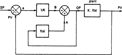
The inverse plant model is usually implemented with a sampled digital system. The problem with this simple, and apparently ideal, controller is that it will probably demand actuation signals which will drive the controller output, the actuator or parts of the plant, into saturation. It also requires an accurate plant model. A more gentle version of this technique aims to get a fraction, say 0.1 of the way from the current value to the desired value of the process variables at each sample time. This approximates to an exponential response.
13.28 Digital control algorithms
So far we have assumed that controllers deal with purely analog signals. Increasingly controllers are digital, with the analog signal from the transducer being sampled by an ADC, the control algorithm being performed by software and the analog output being obtained from a DAC. ADCs and DACs are described in Chapter 14, Section 14.9. The system does not therefore continually control but takes ‘snapshots’ of the system state. Such an approach is called a sampled system.
13.28.2 Shannon’s sampling theorem
A sampled system only knows about the values of its samples. It cannot infer any other information about the signals it is dealing with. An obvious question, therefore, is what sample rate we should choose if our samples are to accurately represent the original analog signals.
In Figure 13.82(a) a sine wave is being sampled at a relatively fast rate. Intuitively one would assume this sampling rate is adequate. In Figure 13.82(b) the sample rate and the frequency are the same. This is obviously too slow as the samples imply a constant unchanging output.
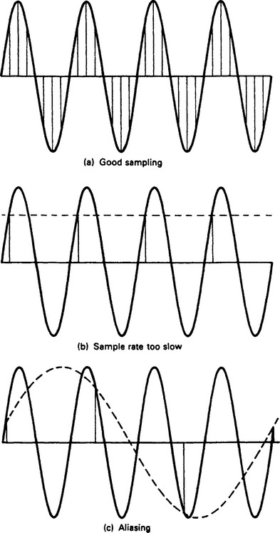
Figure 13.82 The effect of the sampling rate: (a) good sampling rate; (b) sampling frequency same as signal frequency, too slow; (c) sampling rate much too slow, aliasing is occurring
In Figure 13.82(c) the sample rate is lower than the frequency and the sample values are implying a sine wave of much lower frequency than the signal. This is called ‘aliasing’. A visual effect of aliasing can be seen on cinema screens where moving wheels often appear to go backwards. This effect occurs because the camera samples the world at about 50 times per second.
Any continuous signal will have a bandwidth of interest. The sampling frequency should be at least twice the bandwidth of interest. This is known as Shannon’s sampling theorem. Any real life system will not, however, have a well defined bandwidth and sharp cut-off point. Noise and similar effects will cause any real signal to have a significant component at higher frequencies. Aliasing may occur with these high frequency components and cause apparent variations in the frequency band of interest. Before sampling, therefore, any signal should be passed through a low pass anti-aliasing filter to ensure only the bandwidth of interest is sampled.
Most industrial control signals have a bandwidth of a few Hz, so sampling within Shannon’s limit is usually not a problem. Normally the critical bandwidth is not known precisely so a sample rate of about 5 to 10 times the envisaged bandwidth is used.
13.28.3 Control algorithms
To achieve three term control with sampled signals we must find the derivative and the integral of the error. As shown on Figure 13.83 we are dealing with a set of sampled signals, yn, yn−1, yn−2 etc. where yn is the most recent. If the sample time is Δt, the slope is then given by:
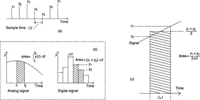
Figure 13.83 Control algorithm with sampled signals: (a) the sampled signals; (b) integration for an analog and digital signal; (c) trapezoid integration
Integration is equivalent to finding the area under a curve as shown for an analog and digital signal on Figure 13.83(b). The trapezoid integration of Figure 13.83(c) is commonly used where the area is given by:
Combining these gives a digital sampled PID algorithm
where en is the error for sample n and Δt the sample time as before.
13.29 Auto-tuners
Tuning a controller is more of an art than an exact science and can be unbelievably time consuming. Time constants of tens of minutes are common in temperature loops, and lags of hours occur in some mixing and blending processes. Performing, say, the ultimate cycle test of Section 13.30.2 on such loops can take several days.
Self tuning controllers aim to take the tedium out of setting up a control loop. They are particularly advantageous if the process is slow (i.e. long time constants) or the loop characteristics are subject to change (e.g. a flow control loop where pressure/temperature changes in the fluid alter the behaviour of the flow control valve.)
Self tuning controllers give results which are generally as good, if not slightly better, than the manual methods of Section 13.30 (possibly because self tuning controllers have more patience than humans!). In the author’s experience, however, the results from a self tuner should be viewed as recommendations or initial settings in the same way as the results from the manual methods described in the following sections. One early decision to be made when self tuners are used is whether they should be allowed to alter control parameters without human intervention. Many engineers (of whom the author is one) view self tuners as commissioning aids to be removed before a plant goes into production.
There are essentially two groups of self tuners. Modelling self tuners try to build a mathematical model of the plant (usually second order plus transit delay) then determine controller parameters to suit the model. These are sometimes called explicit self tuners.
Model identification is usually based on the principles of Figure 13.84. The controller applies a control action OP to the plant and to an internal model. The plant returns a process variable Pv and the model a prediction PVm. These are compared, and the model updated (often via the statistical least squares technique). On the basis of the new model, new control parameters are calculated, and the sequence repeated.
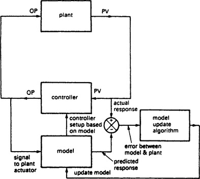
A model building self tuner requires actuation changes to update its model, so it follows that self tuners do not perform well in totally static conditions. In a totally stable unchanging loop, the model, and hence the control parameters, can easily drift off to ridiculous values. To prevent this, most self tuners are designed to ‘kick’ the plant from time to time, with the size and repetition rate of the kick being set by the control engineer. Less obviously, model building self tuners can be confused by outside disturbances which can cause changes in Pv that are not the result of the controller output.
The second group of self tuners (sometimes called implicit tuners) use automated versions of the manual tests described in Section 13.30, and as such do not attempt to model the plant. A typical technique will vary the controller gain until a damped oscillatory response is observed. The control parameters can then be inferred from the controller gain, the oscillation period and the oscillation decay rate.
The useful bang/bang test of Section 13.30.3 can be performed automatically by a controller which forces limit cycling in the steady state via a comparator. A limit block after the comparator restricts the effect on the plant.
Implicit self tuners, like their modelling brothers, do not perform well on a stable unchanging loop, and can be equally confused by outside disturbances.
13.30 Practical tuning methods
Values must be set for the gain and integral/derivative times before a controller can be used. In theory, if a plant model is available, these values can be determined from Nichols charts or Nyquist diagrams. Usually, however, the plant characteristics are not known (except in the most general terms) and the controller has to be tuned by experimental methods.
It should be noted that all these methods require pushing the plant to the limit of stability. The safety implications of these tests must be clearly understood. Tuning can also be very time consuming. With large chemical plants tuning of one loop can take days.
Most of the tests aim to give a quarter cycle decay and assume the plant consists of a transit delay in series with a second order block (or two first order lags) plus possible integral action.
In conducting the tests, it is useful to have a two pen recorder connected to the Pv (process variable) and Op (controller output) as shown on Figure 13.85. The range of the pens (e.g. 0–10 V or 1–5 V) should be the same.
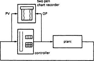
In the tests below, the gain is expressed as proportional band (PB) per cent. Time is used for integral and derivative action. Conversion to gain or repeats per minute is straightforward.
13.30.2 Ultimate cycle methods
The basis of these methods is determining the controller gain which just supports continuous oscillation, i.e. point A and gain K on the Nichols chart and Nyquist diagram of Figure 13.86. The method is based on work by J. G. Ziegler and N. B. Nichols and is often called the Ziegler Nichols method.
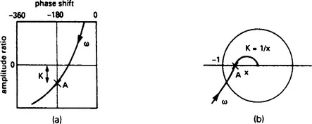
Figure 13.86 Basis of the ultimate cycle test. Point A determines the frequency at which continuous oscillations will occur when gain K is applied: (a) Nichols chart; (b) Nyquist diagram
The integral and derivative actions are disabled to give proportional only control, and the control output manually adjusted to bring Pv near the required value. Auto control is selected with a low gain.
Step disturbances are now introduced and the effect observed. One way of doing this is to go back into manual, shift Op by, say 5%, then reselect automatic control. At each trial the gain is increased. The increasing gain will give a progressively underdamped response and eventually continuous oscillation will result. Care must be taken in these tests to allow all transients to die away before each new value of gain is tried.
If the value of gain is too high, the oscillations will increase. The value of gain which gives constant oscillations neither increasing or decreasing is called the ultimate gain, or Pu (expressed as proportional band). The period of the oscillations Tu should also be noted from the chart recorder (or with a watch).
The required controller settings are:
Ti = 4 Td is a useful rule of thumb.
Other recommended settings for a PID controller are:

All of these values should be considered as starting points for further tests.
13.30.3 Bang/bang oscillation test
This is the fastest, but most vicious, test. It can, though, be misleading if the plant is non linear. Integral and derivative actions are disabled and the controller gain set as high as possible (ideally infinite) to turn the controller into a bang-bang controller. The controller output is set manually to bring the process value near the set point then the controller switch into automatic mode.
Violent oscillations will occur as shown on Figure 13.87. The period of the oscillations To is noted along with the peak to peak height of the process variable oscillations as a percentage Ho% of full scale.
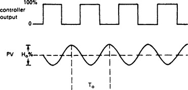
13.30.4 Reaction curve test
This is an open loop test originally proposed by American engineers Cohen and Coon. It assumes the plant consists of a measurable transit delay and a dominant time constant. It cannot be applied to plants with integral action (e.g. level control systems).
A chart recorder must be connected to the plant as shown earlier on Figure 13.85 to perform the test. The controller output is first adjusted manually to bring the plant near to the desired operating point. After the transients have died away a small manual step ΔOP is applied which results in a small change ΔPV as shown on Figure 13.88.
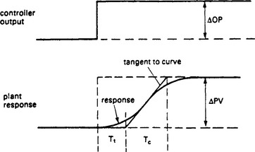
The process gain Kp is then simply ΔPv/ΔOP.
A tangent is drawn to the process variable curve at the steepest point from which an apparent transit delay Tt and time constant Tc can be read. The settings for the controller are then given by:
Because the test uses an open loop trial with a small change in the controller output it is the gentlest and least hazardous tuning method.
13.30.5 A model building tuning method
The closed loop tuning methods described so far require the plant to be pushed to, (and probably beyond), the edge of instability in order to set the controller. An interesting gentle tuning method was described by Yuwana and Seborg in the journal AIChE Vol 28 no 3 in 1982.
The method assumes the plant has gain KM and behaves as a dominant first order lag TM in series with a transit delay DM. This assumption can give gross anomalies with plants with integral action such as level or position controls, but is commonly used for many manual and automatic/adaptive controller tuning methods. With the above warning noted, the suggested controller settings can be found from:
where A, B, C, D, E, F are constants defined:
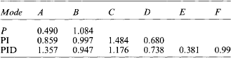
These apparently random equations and constants come from experimental work described by Miller el al in Control Engineering Vol 14 no 12.
The method of finding the plant gain, time constant and transit delay is based on a single quick test with the plant operating under closed loop control. The test is performed on the plant operating under proportional only control, with a gain sufficient to produce a damped oscillation as Figure 13.89 when a step change in set point from R0 to R1 is applied.
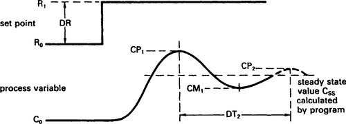
Figure 13.89 Test performed for model building tuning test. Note that Ro and Co need not be the same and DR can be positive or negative
The subsequent process maximum CP1, minimum CM1 and next maximum CP2 are noted along with the time DT2 between CP1 and CP2. The controller proportional band used for the test, PB, is also recorded, from which the controller gain KPB = 100/PB is found.
Given the values from the test the method estimates the value of the plant steady state gain KM, lag time constant TM and the transit delay time DM. The background mathematics is given at length in the original paper.
The equations above are not very practical for manual use on site, so the original paper was developed into a program for the Hewlett Packard HP-67 calculator by Jutan and Rodriguez and published in the magazine Chemical Engineering September 1984. The nomenclature used in the above equations is based on this article.
13.30.6 General comments
The above test procedures do not give guaranteed results and should be viewed as a method of putting the engineer in the right area. They should be viewed as the starting point for further trials. The important thing in these trials is only change one thing at once.
With values set as above the effect of changing the gain should be tried first. It is always useful to have the proportional gain as high as possible to give the largest initial control action to changes and disturbances. However, a large gain can give undesirable changes in the controller output if the process variable is noisy. The gain should be adjusted to give the desired overshoot and damping.
Integral action should be adjusted next to give best removal of offset error. During these trials it is best to disable any derivative action. Decreasing the integral time reduces the time taken to remove the offset error. It may be necessary to reduce the gain again as integral time is decreased. A useful rule of thumb is that the ratio of Ti/Gain is an ‘index’ of stability for a given system, i.e. a Ti of 12 sec and a gain of 2 will give a similar damping to a Ti of 24 sec and a gain of 4.
The derivative action should be adjusted last. Many systems do not benefit from derivative action, particularly those with a noisy process variable signal which causes large controller output swings. Where derivative action is required, Td = Ti/4 is a good starting point. Many controllers allow the user to select derivative action on error or derivative action on process variable. The former is best for tracking systems, but gives large controller output swings for step changes in the set point. Derivative action on process variable is usually the best choice.
One final observation, based on experience rather than theory, is that a PB of 200% (gain of 0.5), Ti of 20 sec and no derivative action is a good starting point for a majority of plants. Adjust the gain to give the required overshoot then adjust Ti to be as small as possible. Finally set Td, if needed, to Ti/4.
1. Saucedo, R., Schiring, E.E. Introduction to Continuous and Digital Control Systems. Macmillan; 1968.
2. Franklin, G.F., Powell, J.D., Emaminaeini, A. Feedback Control of Dynamic Systems. New York: Addison-Wesley; 1986.
The authors have found the following books useful for basic control engineering studies. This list is by no means exhaustive.
Anand, D.K. Introduction to Control Systems. New York: Pergamon Press; 1974.
Chen, C.F., Haas, I.J. Elements of Control Systems Analysis. Oxford: Prentice-Hall; 1968.
Distefano, J.J., Stubberud, A.R., Williams, I.J. Theory and Problems of Feedback and Control Systems. In Schaum’s Outline Series. Englewood Cliff, NJ: McGraw-Hill; 1990.
Dorf, R.C. Modern Control Systems. New York: Addison-Wesley; 1980.
Douce, J.L. The Mathematics of Servomechamsms. New York: English Universities Press; 1963.
Elgard, O.I. Control Systems Theory. London: McGraw-Hill; 1967.
Golten, J., Verwer, A. Control System Design and Simulation. New York: McGraw Hill; 1991.
Healey, M. Principles of Automatic Control. Hodder and Stoughton; 1975.
Jacobs, O.L.R. Introduction to Control Theory. New York: Oxford University Press; 1974.
Langill, A.W. Automatic Control Systems Engineering. In Vols I and II. Oxford: Prentice-Hall; 1965.
Marshall, S.A. Introduction to Control Theory. Englewood Cliffs, N.J.: Macmillan; 1978.
Power, H.M., Simpson, R.J. Introduction to Dynamics and Control. New York: McGraw-Hill; 1978.
Raven, F.H. Automatic Control Engineering. New York: McGraw-Hill; 1961.
Shinskey, F.G. Process Control Systems. New York: McGraw Hill; 1988.