24
Alternative Architectures for NonBoolean Information Processing Systems
Yan Fang1, Steven P. Levitan1, Donald M. Chiarulli11, and Denver H. Dash2
1Department of Electrical and Computer Engineering, University of Pittsburgh, USA
2Intel Science and Technology Center, USA
24.1 Introduction
In this chapter we explore algorithms and develop an architecture based on emerging nano-device technologies for cognitive computing tasks such as recognition, classification, and vision. Though the performance of computing systems has been continuously improving for decades, for cognitive tasks that humans are adept at, our machines are usually ineffective despite the rapid increases in computing speed and memory size. Moreover, given the fact that CMOS technology is approaching the limits of scaling, computing systems based on traditional Boolean logic may not be the best choice for these special computing tasks due to their massive parallelism and complex nonlinearities. On the other hand, recent research progress in nanotechnology provides us opportunities to access alternative devices with special nonlinear response characteristics that fit cognitive tasks better than general purpose computation. Building circuits, architectures, and algorithms around these emerging devices may lead us to a more efficient solution to cognitive computing tasks or even artificial intelligence. This chapter presents several nonBoolean architecture models and algorithms based on nano-oscillators to address image pattern recognition problems.
The idea of special hardware architectures for cognitive tasks is not new. Equivalent circuits for a neuron model go back at least to 1907, where the model was just simply composed of a resistor and a capacitor [1]. Since then, various models have been implemented based on different technologies. In the late 1980s, Carver Mead proposed the term neuromorphic system in reference to all the electronic implementations of neural systems [2]. Meanwhile, with the development of digital computing systems, theoretical and computational models for neural networks and the human brain have been improved and refined many times. From the McCulloch–Pitts neuron model to the Hodgkin and Huxley's model [3,4], computational neuroscience gives us precise mathematic descriptions of the neuron. However, models for a single neuron or synapse have not proved to be good enough to explain the cognitive ability of a whole brain. More recent research trends have focused on the hierarchical structure of human brain and vision system, like Hierarchical Temporal Memory (HTM) [5], Hierarchical Memory and X (HMAX) [6], and so on. With the new opportunities from emerging nano-devices and neuroscience, we can gain insights from both disciplines and design new architectures for cognitive computing tasks based on nonBoolean functions from a more macroscopic view of a hierarchical model of the human brain instead of single neural network.
In this chapter, we build upon this background to take advantage of the unique processing capabilities of weakly coupled nonlinear oscillators to perform the pattern recognition task. In particular, we focus on pattern matching in high dimensional vector spaces to solve the “k-nearest neighbor” search problem. We choose this problem due to its broad applicability to many machine learning and pattern recognition applications. Taking the image recognition problem as an example, we can choose whether or not to preprocess an image using feature extraction. If we choose not to perform preprocessing, the image itself can simply be considered as a long feature vector. Either way, the feature vectors of the image need to be compared with some memorized vectors and matched to the “nearest neighbor” in the feature vector space for recognition.
In the rest of this chapter, we first introduce the concept of an associative memory (AM) and Oscillatory Neural Networks and implement their function by using a traditional well-understood electronic device, the phase-locked loop (PLL). Next, we explain the structure of an AM unit based on nano-oscillators and show how to deal with patterns in high dimension vector spaces by partitioning them into segments and storing them in multiple AM units. Then, we propose two hierarchical AM models that try to address pattern matching problems in both high dimensions and for large data sets. The first hierarchical structures organize AM units into a pyramid. The image patterns are separated into different receptive fields and processed by individual AM units at the low level, and then abstracted at higher levels of the model. The second hierarchical model for the AM architecture is developed for large data sets. In this model, AM units are nodes of a tree, and patterns are classified by hierarchical k-means clustering algorithms and stored in the leaf nodes of the tree, while other nodes only memorize centroids of clusters. During the recognition process, input patterns are compared with cluster centroids and classified to subclusters iteratively until the correct pattern is retrieved.
24.1.1 Associative Memory
An associative memory is a brain-like distributed memory that learns by association. Association has been known to be a prominent feature of human memory since Aristotle, and all models of cognition use association in one form or another as the basic operation [7]. Association takes one of two forms: auto-association or hetero-association. Auto-associative memory is configured to store a set of patterns (vectors) and is required to be able to retrieve the original specific pattern when presented with a distorted or noisy version. In other words, when the input pattern is different from all the memorized patterns, the AM retrieves a best match to the input pattern given some distance metric, like the Euclidian distance. Thus, the association is a nearest neighbor searching procedure.
As an example shown in Figure 24.1, consider an auto-associative neural network that has memorized three binary image patterns for the numbers “0,” “1,” and “2.” When a distorted image “1” is fed into the network, the output pattern should be the stored image “1,” which is the closest pattern in this associative memory.

Figure 24.1 Example of image pattern retrieval
Hetero-associative memory is the same except its output patterns are coded differently from the input patterns. Therefore, we can consider that a mapping between input and output patterns is stored in the network for pattern retrieval. Hetero-association happens in many cognitive procedures. For instance, a group of neurons in one region of the brain activates neurons in multiple cortical regions.
In its simplest form, associative memory operations involve two phases: storage and recall. In the storage phase, we train the network with patterns by following a particular rule (e.g., a Hebbian learning rule, or a Palm rule) that can form a weight matrix which indicates the weights of connectivity between neurons. Therefore, in the training stage, the network stores the patterns we need in the interconnection weights. In the recall phase, the network performs pattern retrieval by using the interconnection weights to process a possible noisy version of one of the stored patterns. It is assumed that the input pattern is based on one of the stored patterns.
The number of patterns stored in the associative memory provides a direct measure of the storage capacity of a network. In the design of an associative memory, the tradeoff between storage capacity and correctness of retrieval is a challenge [7].
The earliest AM model explored by Steinbuch and Piske in the 1960s [8] was called Die Lernmatrix. It represents patterns with binary vectors and uses the Hebbian learning rule. Based on this model, Willshaw's group improved its information capacity with sparsely encoded binary vectors and proposed a model called an “Associative Net” [9,10]. They also tried to explain some brain network functions such as short-term memory with their model [11]. In the 1980s Palm proved the storage capacity of Willshaw's model by a different method. Palm improved his model by introducing real-value weights and an iterative structure. Brain state in a box (BSB) is another AM model proposed by Anderson's group [12,13]. In 2007 the “Ersatz Brain Project” utilized BSB in building parallel, brain-like computers in both hardware and software [14]. The Hopfield network invented by John Hopfield in the 1980s included the idea of an energy function in the computation of the recurrent networks with symmetric synaptic connections [15]. The most important contribution of the Hopfield Network is that it connects neural networks with physics and the method of analyzing network stability from the viewpoint of a dynamic system.
24.1.2 Oscillatory Neural Networks
We base our AM model design on the work of Hoppensteadt and Izhikevich that studied weakly connected networks of neural oscillators near multiple Andronov–Hopf bifurcation points [16]. They propose a canonical model for oscillatory dynamic systems which satisfy four criteria:
- Each neural oscillator comprises two populations of neurons: excitatory neurons and inhibitory neurons.
- The activity of each population of neurons is described by a scalar (one-dimensional) variable.
- Each neural oscillator is near a nondegenerate supercritical Andronov–Hopf bifurcation point.
- The synaptic connections between the neural oscillators are weak.
Given these conditions, this canonical model can be represented by the function:
Where:
| • |
Complex oscillator variable |
| • |
Damping of oscillators |
| • |
Natural frequencies of oscillators |
| • |
Nonlinear factor, ensures stable amplitude |
| • |
Coupling parameter, typically small (weakly coupled) |
| • |
Coupling matrix, represent coupling strength between two oscillators similar to the weight matrix in previous models |
This dynamic model was proved to be able to form attractor basins at the minima of a Lyapunov energy function by adjusting the coupling matrix though a Hopfield rule [15]. In other words, a network that consists of oscillators described by this canonical model can learn patterns as represented by phase errors and perform the functions of an associative memory.
An example of Oscillatory Neural Network that shares the same structure as a recurrent feedback Hopfield network is depicted in Figure 24.2.
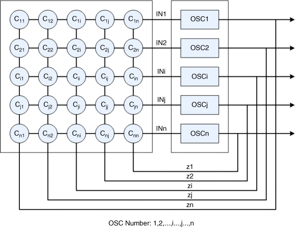
Figure 24.2 Oscillatory neural network structure
The oscillator cluster (OSC1, OSC2, OSC3,…, OSCn) are coupled by a matrix of multipliers and adders that contain the coupling coefficients, shown as the Cij box. The outputs are fed back to the network as the coupling term of Equation 24.1 for the recurrent evolution process until the network state is completely stabilized at an attractor.
Hoppensteadt and Izhikevich's Oscillatory Neural Network model demonstrates a similar functionality and dynamic behavior as the Hopfield Network [15]. An example of Oscillatory Neural Networks serving as an AM model is presented in the next part of this section.
24.1.3 Implementation of Oscillator Networks
To illustrate how to implement an Oscillatory Neural Network in hardware, we choose the example of an oscillator network composed of phase-locked loops [17]. The behavior and structure of this simple network helps to understand how Oscillatory Neural Networks can store and retrieve patterns.
A phase-locked loop is a device that generates an output signal whose phase is related to the phase of an input “reference” signal. As Figure 24.3 shows, it consists of a voltage-controlled oscillator and a phase detector implemented as a multiplier and low pass filter.

Figure 24.3 Structure of phase-locked loop
This circuit compares the phase of the input signal with the phase of the signal derived from its output oscillator and adjusts the frequency of its oscillator to keep the phases matched. The signal from the phase detector is used to control the oscillator in a feedback loop. Frequency is the derivative of phase, therefore, keeping the input and output phase in lock step implies keeping the input and output frequencies in lock step. Consequently, a phase-locked loop can track an input frequency, or it can generate a frequency that is a multiple of the input frequency.
A network of PLL circuits can form a structure similar to the canonical oscillator network described above. The input signal of each PLL is the weighted sum of the outputs of every PLL, including itself. The only additional operation is that there is a π/4 delay in the feedback loop to make the input signals and reference signals inside the PLL orthogonal.
By simulation in Matlab, we can observe the properties of the PLL network more directly. We have built the model with the following parameters:
| • N = 64 | Number of oscillators |
| • f = 1000 | Natural frequency of VCO (Hz) |
| • d = 1/(f*100) | Simulation step size |
| • T = 0.5 s | Simulation time |
| • sens = 100 | Sensitivity of VCO |
| • amp = 1 | Amplitude of VCO output |
| • Kd = 1 | Gain of phase detector |
As an example of the operation of this model we can store two patterns, the 8 × 8 images of “1” and “5” and observe the convergence behaviors of the array. In Figure 24.4 we use a random binary image (as a “very noisy” input), start the simulation, and observe the evolution process of the phase behavior of the oscillators. The system converges to the closest stored pattern, which is “5” in this case.
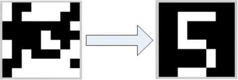
Figure 24.4 Binary image pattern retrieval in a PLL network
We plot the phase error between the oscillators in terms of their cosine value. In Figure 24.5 we see the time evolution of the phase error.
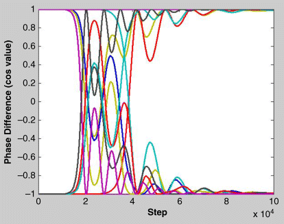
Figure 24.5 Evolution of the phase error in a binary image pattern retrieval process
In a second test, we give the system a random gray scale image, which means that the initial condition is not fixed to binary values. Similarly, Figure 24.6 and Figure 24.7 show the retrieval process.
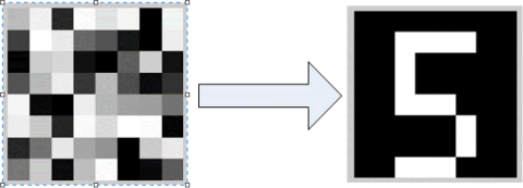
Figure 24.6 Grayscale image pattern retrieval of PLL network

Figure 24.7 Evolution of the phase error in grayscale image pattern retrieval process
From the experiments above, we suggest that the phase-locked loop, as both a model and an implementation for the basic neuron of oscillatory neural network, is able to behave as a canonical oscillator model. However, it is costly in terms of hardware resources compared with several novel devices presented later. It also has a slow convergence speed. In fact, based on our experiments, the PLL networks that use the Palm coding rule does not always converge.
Compared to the PLL, other oscillator circuits could be better choices for building an AM model, for instance, oscillators based on the Neuron MOS or the spin torque nano-oscillators (STNO). The Neuron MOS transistor is a type of MOS transistor that has multiple floating gates used to model a neuron [18]. In a simple CMOS ring oscillator, an inverter consisting of neuron PMOS and NMOS transistors has an input voltage capable of controlling the delay of signal propagation and thus changes the oscillating frequency [19]. The STNO is an emerging nano-device that can also be used to implement an oscillator AM model. STNOs work on injection of high density current into multiple magnetic thin layers. Current-driven transfer of angular momentum between the magnetic layers in such a structure results in spontaneous precession of the magnetization once the current density exceeds the stability threshold. This magnetization precession generates microwave electrical signals as a result of an effect called giant magneto-resistance (GMR) that occurs in such magnetic multilayer structures [20]. STNOs demonstrate the functionality associated with VCOs, including frequency modulation and injection locking [21,22]. Given these characteristics, STNOs can couple with each other either by mutually locking on phase or by shifting each other's frequency.
Different from the structure of PLL-based oscillatory neural networks with fully connected feedback (Figure 24.2), these oscillators are designed to couple together through one node and thus form a cluster, as shown in Figure 24.8. A cluster model composed of such nano-oscillators needs no complex feedback connection matrix. Each oscillator is sensitive to all others and can simultaneously influence them without coefficients computed from multipliers and adders. Further, the number of interconnects scale as N rather than N2. However, even for this much simpler network, the dynamic behavior of these oscillators is still determined by the energy function of the network.
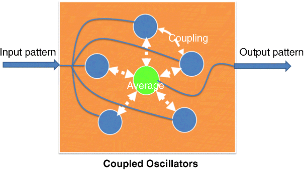
Figure 24.8 Coupled oscillators cluster
A new AM unit can be designed with supportive circuits around such nano-oscillator clusters. Figure 24.9 depicts a simple structure of such an AM unit. This model's architecture is designed like a Content Addressed Memory (CAM). It is composed of multiple “Associative Words” that contain nano-clusters with local template memories and code memories, write/match control circuits, and circuits for output. As a hetero-associative memory, the template memory and code memory respectively store the memorized pattern and their code representations. Write/Match control circuits control the modes and operation of the AM unit. It has three input signals; an input pattern Xi, the code representation Ci for new stored pattern, and the model control signal. The circuits for output detect all the degrees of match (DoM) from each oscillator cluster and return the maximum DoM, d*, with the corresponding winner pattern's code, Ci, as the final outputs of the recognition process.
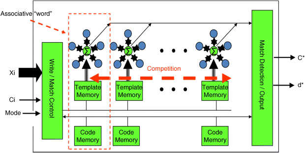
Figure 24.9 AM unit built on coupled oscillator clusters
This AM unit has two modes, Write and Match. In the Write mode, it stores each new pattern in the local template memory of each cluster. In the Match mode, the oscillator clusters read the differences between the input pattern and stored patterns, and then outputs the (DoM). Thus, the result for pattern recognition will be the pattern within the cluster which outputs the maximum DoM.
In the binary domain, this AM unit model can be abstracted as a simple Palm Network Model with all the patterns sparsely represented by unary codes [23]. However, in the real number domain, the oscillator clusters utilize a quite different distance metric based on the nano-oscillator's nonlinear behavior for matching.
From the perspective of nano-device technology, it may be difficult to couple a large number of nano-oscillators together, and we do not yet know about the capacity of an AM model in such a cluster structure. However, compared to the structure of traditional recurrent feedback neural networks implemented on hardware, the advantages of this AM cluster design for nano-oscillators includes fewer wires and connections, lower memory costs, and shorter convergence time.
24.2 Hierarchical Associative Memory Models
In the previous section, we have shown that weakly coupled oscillatory neural networks are capable of memorizing multiple patterns and retrieving the “closest” one to an input pattern. Taking this idea one step further, we believe that oscillatory neural networks can also perform the functions of the Palm model and form a complete associative memory system.
Nevertheless, there still exist many technical problems when novel oscillatory devices are used to form large-scale neural networks. Full connection within the associative memory requires the full and tuned connection of oscillators within the network, which is difficult for coupling between nano-scale oscillators. Even if we can build a large “flat” neural network, the maximum efficiency of a fully connected Palm model can only reach 35% [22]. Compared with a biological neural system, this type of model has a very low efficiency.
On the other hand, hierarchical structures have been identified in the neocortex of human beings and this area of the brain is believed to perform the functions of memory retrieval and logical inference [24]. We can hypothesize that a large number of associative memories are organized hierarchically in this structure. For both these reasons, we have investigated the design of a hierarchical associative memory system made by connecting Palm models.
24.2.1 A Simple Hierarchical AM Model
Figure 24.10 illustrates a three-level hierarchical model that can memorize 8 × 8 binary images (64 bits in total). As Figure 24.10 shows, each AM unit (X1…X4, Y1, Y2, and Z1) represents one Palm network with 16 input neurons and eight output neurons. Every AM unit in a higher level receives the output of two units from the lower level. The training patterns and the test patterns are sliced into four pieces (shown with red lines) and are respectively fed into the four “X” modules in the bottom level.
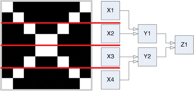
Figure 24.10 Three-level hierarchical structure and receptive field
The hierarchical model is trained from lowest level (X level) to the highest level (Z level) either using the Palm model's training rule [22] or by writing the patterns directly into the memory. After each lower level is trained, it feeds its output vectors as the training vectors to the next higher level. Therefore, eventually, every AM unit learns the patterns of its receptive field (the fraction of the pattern under it in the hierarchy) and builds the input–output mapping function to generate a corresponding output vector. The pattern retrieval task, like the training task, is processed sequentially. In this case, we put a distorted image pattern into the X level. The AM units at the X level will output unary codes to the Y level, which will then generate output codes, and the module at the Z level will recognize the whole pattern based on the Y level outputs. To more closely model the behavior of a hypothetical Palm network built from oscillatory neural networks, we adjusted the Palm model in its retrieval process. Instead of using a Heaviside function and threshold as the output, we take a “winner take all” (WTA) strategy. In this technique, the DoM is obtained by comparing two binary vectors with the bit-OR operation like a Palm model, which indicates the similarity between the input pattern and each memorized pattern. And, the pattern with the highest DoM is the winner. All other patterns will be “losers.” A winner is randomly picked when multiple patterns have the same highest DoM.
In our tests, we use a unary code for the output pattern of each AM unit and train the system with four simple image patterns labeled P1 to P4 in Figure 24.11.

Figure 24.11 Binary image patterns for first level of hierarchical palm network
To test if the hierarchical model would function as expected, we input many random binary images into the model and observed the retrieval process of each AM unit. One illustrative example of this retrieval process is shown in Figure 24.12 and Figure 24.13. In this case, the random image shown in Figure 24.12 is recognized as an “X.”

Figure 24.12 Input pattern and output pattern in function test for hierarchical model
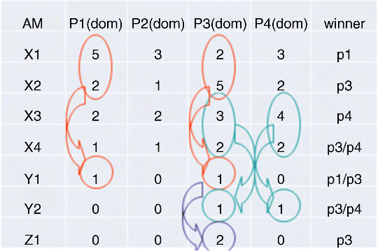
Figure 24.13 Function test retrieval process
Figure 24.13 explains the retrieval process of all the AM units in the hierarchy for the test in Figure 24.12. In this figure, the first column contains the name of all the AM units. The middle four columns give the DoM between the input pattern and each stored pattern from the perspective of each different AM unit. And the winner column shows the decision made by these AM units based on the DoM they generate. The circles and arrows explain how the higher levels compute the winner pattern through the information from lower levels. For example, X1 finds the local maximum DoM within its own receptive field is five, generated from pattern p1, and thus outputs p1 as the winner pattern, while X2 does the same thing but gets a different result, p3. Y1 reads the output from X1 and X2, and then puts the DoM from p1 and p3 equally to 1. Therefore, “1010” will be Y1's output. Similarly, the top AM unit Z1 makes the final decision of the system after reading the output from Y1 and Y2. It picks the third pattern p3 as the result of this retrieval process. If we only look at the DoM output from the bottom level and sum them up for each pattern, the DoM of direct comparisons from a single AM unit can be obtained. They are 10, 7, 12, and 11, respectively for p1 to p2. Obviously p3 will also be the winning pattern with the highest DoM.
After the hierarchical model's ability to retrieve patterns was verified, we still needed to test whether the patterns retrieved met our expectations of finding the “right” pattern that is in agreement with our human perception. Hence, we developed a “robust test” where we used an input pattern with some part of the pattern exactly the same as a trained pattern and some part of the receptive field distorted. Figure 24.14 presents the recovery of two such distorted patterns and the DoM of each Palm network as the recognition process proceeds.
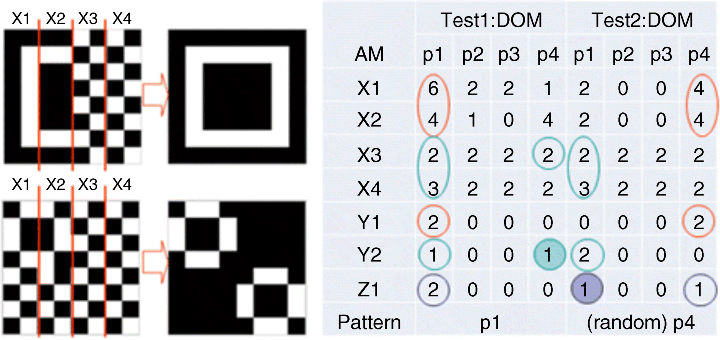
Figure 24.14 Robust test for hierarchical model
These simulation results show that this simple hierarchical AM model can memorize and retrieve patterns with results similar to a large single “flat” associative memory as a nearest neighbor classifier.
24.2.2 System Improvements
The simple model we discussed above illustrates the first step of our exploration of hierarchical AM architectures. However, as we explain below, there are several deficiencies in this model. We next provide an analysis of these problems and provide corresponding solutions as improvements to the AM system.
24.2.2.1 Pattern Conflict
During the pattern retrieval process, when the lower level's AM units output different patterns with the same DoM, the system sometimes performs recognition poorly due to the random choice for tie breaking. In the case shown in Figure 24.15, the correct pattern should be p1. But the AM units in the second level and top level randomly pick a pattern between p1 and p3 because they have the same DoM in the local AM unit. Since the AM units in the same layer are independent and cannot communicate with each other, the AM unit from the higher layer receives incomplete information and thus retrieves an incorrect pattern. We define this phenomenon as Pattern Conflict, which reflects the weakness of the hierarchical AM model structure in passing and abstracting global information. Without more connections between networks, associative information from different receptive fields is lost from the lower levels to the higher levels.
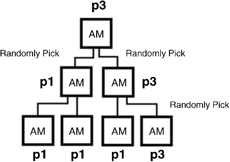
Figure 24.15 Example of the pattern conflict case
24.2.2.2 Difficulty in Information Abstraction
In an ideal hierarchical structure, the higher level input vectors are the concatenation of lower level modules' input vectors to prevent information loss. Thus, the size of the network increases as one goes to higher levels. Unfortunately, the oscillator AM module cannot be very large due to the practical considerations of implementing large networks. Therefore, if we keep all the AM units the same size, the output patterns from the lower levels to the higher levels have to be abstracted into shorter vectors which causes a loss of the input pattern's original information.
24.2.2.3 Capacity Problem
In real applications, a hierarchical AM system may be required to memorize a large number of patterns. Since we cannot store all patterns in a single AM module, and we have fewer AM units in the higher level of a hierarchical model, the capacity problem becomes increasingly serious. Given the fact that the top level has only one AM unit, it cannot store as many patterns as the bottom level. In addition, for an oscillator network, more patterns usually mean lower speed and lower accuracy.
24.2.2.4 An Improved Hierarchical AM Model
We solve these problems described above by modifying our hierarchical design in three ways: structure, representation, and training rule. We keep the hierarchical design but change the receptive field of each block, as Figure 24.16 shows. Consider the input image as a 64 × 64 matrix, every module receives the input of a 2 × 2 square area from its lower level. The bottom Level (L1) slices the input image into 16 × 16 blocks and each block has 4 × 4 pixels. This design is better at resisting distortions and noise in the image pattern than the earlier structure.
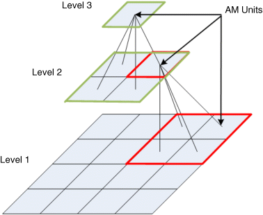
Figure 24.16 Pattern representation between layers
To keep every AM module the same size, the output vectors of the four AM units are translated into a binary code and concatenated to the input vector that is fed to higher levels. In this case, each AM unit can memorize 16 16-bit binary vectors. Their outputs are coded into a four-bit vector and fed to the next level, as shown in Figure 24.17.
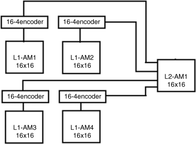
Figure 24.17 Encoders between two layers in the hierarchical model
The function of the 16-4 encoder is to convert the output of the 16-bit unary code into a four-bit binary code. The original 16-bit unary code indicates the index of the output pattern. To obtain the DoM, we use the XNOR operation instead of the multiplication in the Palm model. Figure 24.18 provides an example of how the AM unit recognizes patterns. Here the DoM is measured by the Hamming distance between the input pattern and each of the stored patterns. The unary code output has a single “1” at the index of the highest DoM.
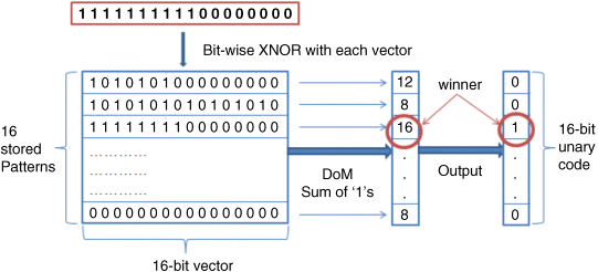
Figure 24.18 AM units function in the hierarchical model
24.2.3 Simulation and Experiments
After making these changes, we test the performance of our improved system. For these tests, we randomly pick 16 64 × 64 images that were converted to binary images from JPEG color pictures, as presented in Figure 24.19. Two sorts of input patterns are used for each of two tests, the first one is the original image with added noise, and the second one is a combination of different parts of two images. In these two tests, the hit rate is defined as the number of trials that our model retrieves the correct pattern divided by the total number of trials. The hit rate represents the ability of the model to perform pattern matching.
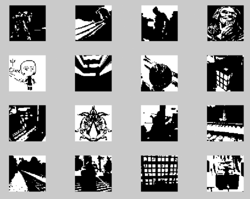
Figure 24.19 Binary image set in pattern retrieval test
24.2.3.1 Noisy Pattern Retrieval Test
In the noisy pattern retrieval test, we randomly choose a percentage of image pixels and flip their value. This sort of noise is added to every image in the data set. Figure 24.20 shows the two examples of 25% noise added to an image. For this amount of noise, it is even hard for a human to recognize these patterns.
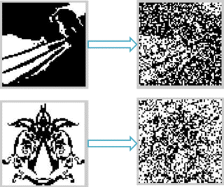
Figure 24.20 Two examples of 25% noise in the noise retrieval test
We vary the noise percentage from 0 to 50% and run each simulation 500 times for each pattern under different noisy inputs. We observe the hit rate of each simulation. Figure 24.21 gives the hit rate for all 16 patterns. We can see that even for a relatively high degree of noise, the hierarchical AM model performs quite well.
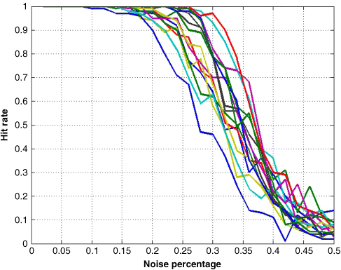
Figure 24.21 Hit rate versus noise degree in noise retrieval test
24.2.3.2 Pattern Conflict Test
To test if the Hierarchical AM model solves the pattern conflict problem, we intentionally combine two images by replacing some columns of one image by another's. In the simulation, we vary the replacement ratio from 10 to 50% and use 16 different patterns to interfere with the fourth pattern. The curves of hit rates and replacement ratios are shown in Figure 24.22. From this result we find that this model reduces pattern conflicts as we expect.
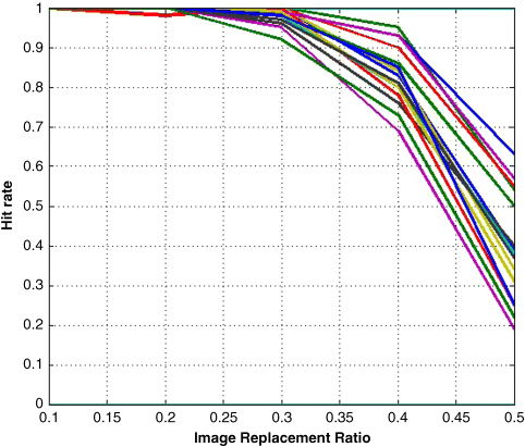
Figure 24.22 Replacement ratio versus hit rate in patten conflict test
24.2.3.3 Pattern Storage
Figure 24.23a–d presents us with the utilization of storage space from the bottom level of hierarchy to the second level from the top. We did not show the top level because we know the top level has only one AM unit and stores all 16 patterns. The heights and colors of the 3-D bars indicate how many patterns each AM unit memorized for this data set. The color bar gives the color code of these four graphs from violet (0) to red (16). The maximum bar height is 16, which is the total capacity of the AM unit, represented with red. The x and y axis show the position of a module in the AM array of each layer. As we expected, AM units in the lower levels store fewer vectors than AM units in a higher level because some images share the same pattern in a small receptive field. For this test, both level 1 and level 2 run out of storage, we cannot memorize more patterns without changing the size of the AM unit. This illustrates a fundamental problem of the associative memory. If we choose to perform a direct comparison between a set of memorized patterns and an input pattern, the system must scale to accommodate all the patterns. However, it is not practical to build such a large monolithic AM unit. Therefore, in the next section, we investigate a new hierarchical architecture and algorithm which allows us to support large data sets.
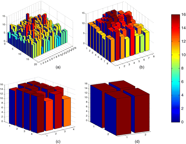
Figure 24.23 The memory usage of each layer of the hierarchical model
24.3 N-Tree Model
To address the fundamental capacity problem that stems from the need for direct comparisons between the input and the data set, we introduce the N-Tree model [25]. In this model, we perform indirect comparisons between the input and representative patterns for subsets of the data. We also investigate the use of branch and bound search to improve the performance of this model.
24.3.1 N-Tree Model Description
The Hierarchical AM model we investigated above does not solve the capacity problem because it only partitions the pattern vectors and compresses them. The input pattern still has to be compared with all the memorized patterns for the nearest neighbor search. Therefore, it is difficult to scale and cannot effectively handle large data sets in high dimension spaces, since both the number and length of vectors grow. Given the fact that a tree structure always contains the least information in its root node and the most information in the totality of its leaf nodes, we reconsider the organization of the data set and propose another model called the N-Tree model.
24.3.1.1 Model Structure
Assume there is a pattern set with m patterns, ![]() , required to be memorized by an AM system. When the number of patterns, m, is very large, it becomes difficult for a single AM unit based on oscillators to hold all the patterns. As discussed previously, this is due to both fabrication and interconnects symmetry constraints. In order for the oscillators to work correctly as a pattern matching circuit, the oscillators need to be matched in performance and the interconnect needs to be symmetrical. Both of these goals can only be reliably achieved if we keep the clusters of oscillators relatively small. Therefore, as a solution to this problem we use a hierarchical AM model that organizes multiple AM units into a tree structure.
, required to be memorized by an AM system. When the number of patterns, m, is very large, it becomes difficult for a single AM unit based on oscillators to hold all the patterns. As discussed previously, this is due to both fabrication and interconnects symmetry constraints. In order for the oscillators to work correctly as a pattern matching circuit, the oscillators need to be matched in performance and the interconnect needs to be symmetrical. Both of these goals can only be reliably achieved if we keep the clusters of oscillators relatively small. Therefore, as a solution to this problem we use a hierarchical AM model that organizes multiple AM units into a tree structure.
If each AM unit can only store n patterns, while ![]() , then the m patterns can be clustered hierarchically into an N-Tree structure and stored in an AM model with the corresponding architecture. In this tree structure, every node is an AM unit and has at most n children nodes. Only leaf nodes (nodes that have no children) store specific patterns from the original input set:
, then the m patterns can be clustered hierarchically into an N-Tree structure and stored in an AM model with the corresponding architecture. In this tree structure, every node is an AM unit and has at most n children nodes. Only leaf nodes (nodes that have no children) store specific patterns from the original input set: ![]() . The higher nodes are required to memorize the information associated with different levels of pattern clusters. Thus, every search operation, to retrieve one pattern, results in a path in the tree from the root to a leaf. During the retrieval process, the key pattern is input recursively into the AM nodes at a different level of the tree and finally the pattern with the highest DoM is output.
. The higher nodes are required to memorize the information associated with different levels of pattern clusters. Thus, every search operation, to retrieve one pattern, results in a path in the tree from the root to a leaf. During the retrieval process, the key pattern is input recursively into the AM nodes at a different level of the tree and finally the pattern with the highest DoM is output.
For example, if we take the simple case where m = 8, n = 2, this case forms the binary tree AM model shown in Figure 24.24. At the root node, patterns are clustered into two groups, ![]() and
and ![]() , respectively, associated with two representative patterns: C11 and C12. There are several ways that the C patterns can be generated during training, as explained below. From the second level, these two groups of patterns are split again into four groups and are stored in four AM units in the third level. In effect, each AM node has an associated pattern, C, stored in its parent node which represents the patterns in its local group.
, respectively, associated with two representative patterns: C11 and C12. There are several ways that the C patterns can be generated during training, as explained below. From the second level, these two groups of patterns are split again into four groups and are stored in four AM units in the third level. In effect, each AM node has an associated pattern, C, stored in its parent node which represents the patterns in its local group.
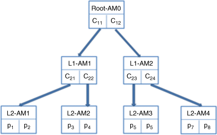
Figure 24.24 Three layers N-Tree model with fanout = 2
24.3.1.2 Training Process
Once the hierarchical structure of the AM model is fixed, the next question is how to organize the patterns into a tree structure and which features can be used for the recognition at each node? These questions determine the method of training and pattern retrieval. Notice the fact that the AM unit always outputs the pattern with the highest DoM, namely the one nearest to the input pattern in the data space. For this work, we use a hierarchical k-means clustering algorithm.
k-Means clustering [26] is a method of cluster analysis which aims to partition n patterns into k clusters in which each pattern belongs to the cluster with the nearest mean. Since these are multi-dimensional means, we also refer to them as “centroids.”
The steps of the algorithm can be summarized as:
- Randomly select k data points (vectors) as initial means (centroids).
- Assign every other data point in the training set to its closest mean (Euclidian distance) and thus form k clusters.
- Recalculate the current mean of each cluster based on all the data points that have been assigned.
- Repeat (2) and (3) until there are no changes in the means.
Hierarchical k-means clustering is a “top-down” divisive clustering strategy. All patterns start in one cluster and are divided recursively into clusters by clustering subsets within the current cluster as one moves down the hierarchy. The clustering process ends when all the current subsets have less than k elements, and they are nondividable. This algorithm generates a k-tree structure that properly matches our AM structure. The internal nodes are centroids of each cluster in different levels and the external nodes (leaf nodes) are exact patterns. During the clustering process, some clusters may become nondividable earlier than others and, therefore, have higher positions in the tree than the other leaf nodes.
Consider the previous example, the first clustering generates two clusters, ![]() and
and ![]() , with centroids C11 and C12. Then these two clusters are split into four subclusters,
, with centroids C11 and C12. Then these two clusters are split into four subclusters, ![]() ,
, ![]() ,
, ![]() , and
, and ![]() . Their centroids are C21, C22, C23, and C24. Since the number of patterns in one cluster is less than the threshold, we set (
. Their centroids are C21, C22, C23, and C24. Since the number of patterns in one cluster is less than the threshold, we set (![]() ) and the clustering process ends. After the centroids and patterns are written into each AM node correctly, the training process is finished.
) and the clustering process ends. After the centroids and patterns are written into each AM node correctly, the training process is finished.
24.3.1.3 Recognition Process
The pattern retrieval process starts from the root node. When we input the pattern that needs to be recognized, the AM unit at the root node will output the nearest centroid as the winner. This centroid will lead to a corresponding node in the next level and the system will repeat the recognition process until the current node is a leaf node. The final output is a stored pattern rather than a centroid. Considering the same example as above, assume we have a test pattern ![]() , which is closest to
, which is closest to ![]() . The retrieval process is:
. The retrieval process is:
- Input
 to the root node AM0, the output pattern is C12, which points to the AM2 of level 1, with the cluster
  .
. - Input
 to L1-AM2, the output pattern is C23, which points to the AM3 of level 2, with the cluster
  .
. - Input
 to L2-AM3, the final output pattern is
  .
.
In general, the N-Tree model reduces the steps of comparison by locating the input pattern in different clusters. Also, this architecture makes an AM system capable of scaling up or down as the data set changes. We only need to vary the tree structure of the data set.
24.3.2 Testing and Performance
In this section, we use two image data sets to evaluate the performance of the N-Tree model. The first data set is from the ATT Cambridge Image Database [27]. This data set contains 400 grayscale images of human faces. These images are photos of 40 people with 10 views for each person. The original images have 92 × 112 pixels with 256 gray levels.
We convert the image size into 32 × 32 and normalize the intensity of all the images by the following method:
- Calculate the means of the grayscale values of all pixels for each image, (
 ).
). - Calculate the mean of all images' pixels, (
 ),
),  .
. - For the i-th (1< = i< = 400) image, every pixel is scaled by multiplying the factor
 so that all the images in the data set are normalized to the same intensity.
For the tests in this section, we do not use any image processing techniques, like feature extraction, to preprocess these images. Rather, the pixel values of an image, or centroid, are directly stored as one vector in our AM model. The purpose of the normalization of size and intensity is to make all pattern vectors fit our model.
In these tests we define the size of our AM unit as 16 × 1024. One AM unit can store 16 images and each image has 1024 (32 × 32) pixels. Thus the nodes of the tree structure can have at most 16 child nodes, instead of two in the example above. The definition of the algorithms in terms of both the training and recognition process remain unchanged.
In this task, the N-Tree model is required to recognize the person in the input image after training. We use a hierarchical version of the ARENA algorithm, a simple, memory-based algorithm for face recognition algorithm [28], which performs nearest neighbor search with a reduced-resolution face image. For evaluation, first, we split the data set into two parts, a training data set and a test data set. The partitioning is based on the subjects. For each subject, we pick nine images for training and one for test. Thus there are 360 images in the training data set and 40 images in the test data set.
After the tree structure has been built from the 360 images, we input images of the test data set sequentially. If the output image and the input image belong to the same subject (from different views) we say the recognition is successful, otherwise we call it a failure. The “hit rate” of this simulation is computed based on the 40 test results, one per subject.
In order to evaluate the system's performance, we use a cross-validation technique [29]. For each run, we randomly pick images for training and for test of each subject such that the model is trained and tested on different data set every time. One example of this partitioning is shown in Figure 24.25. We performed 1000 runs each with a different partition.
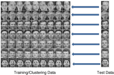
Figure 24.25 Part of ATT data set partitioned for training and testing
This testing environment allowed us to examine two questions. First, what is the influence on performance brought by different norms used in the nearest neighbor search? And second, how good is our hierarchical model's performance compared with a single AM module? Each of these questions is fundamentally important to understand the capability of the N-Tree. Because we have no precise model of a distance metric for the behavior of coupled nano-oscillators, we use several different norms to test in our model. Moreover, since the retrieval performance depends on both the data set and the algorithm we use, our goal is to achieve the performance as an ideal single AM.
To gain some insight into the qualities of different norms, we tested different distance metrics for both the k-means clustering and the searching processes. The model was tested using an L2 norm, L1 norm, and L0 norm respectively.
The L2 norm is the Euclidean distance. On an n-dimensional vector space, the distance between two vectors x and y can be defined as:
The L1 norm is also known as city block distance, or Manhattan distance, which is defined as:
Similarly, the L0 norm is defined as:
![]() is a customized threshold that is determined by the data set in this case.
is a customized threshold that is determined by the data set in this case.
For comparison between our hierarchical methods and a direct implementation of ARENA, we assume we have an ideal single large AM unit that can hold all 360 images and can classify each input image by directly comparing the DoM to every memorized image. This model represents the best performance possible using pixel by pixel distance to classify the face image data.
The results of these tests are summarized in Figure 24.26. It gives the average hit rates and standard deviations of the N-Tree model and the ideal single AM module under different norms. While the standard deviations of all these tests are very small compared to the average hit rates, the N-Tree model's standard deviations are larger than the single AM module because different training data sets generate different trees of data clusters, which directly influences the performance of retrieval. Considering the three different norms, the L0 norm is the best distance metric for nearest neighbor search, while the L1 norm is the second, and the L2 norm is the worst. However, the L0 norm performs the worst for N-Tree model, because it is not a good norm for the k-mean clustering algorithm and thus leads to a bad data clustering.
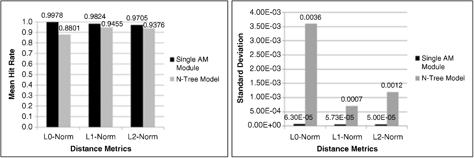
Figure 24.26 Retrieval performance on ATT data set
For the ATT data set, when compared to an ideal “flat” single AM model, our N-Tree model is very close to the best performance with a higher efficiency. Even though the AM performs its comparisons in parallel for each case, the large single AM model has to compute the DoM for all of the 360 stored images, while the N-Tree hierarchical model with a three-level depth performs at most 3 × 16 = 48 operations of comparison with a time penalty of only 3×.
After verifying our model's functionality as an AM system, we employ the same noise test as we used in the previous section to examine the performance of the N-Tree model on a different real application. Salt and pepper noise is a form of noise typically seen on images. It appears as randomly occurring white and black pixels. We keep the training data set and test data set unchanged but make noisy input images by adding salt and pepper noise to test images with a density ranging from 0 to 0.5. Figure 24.27 shows different levels of noise density.
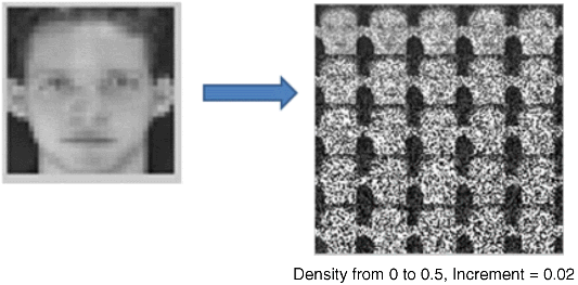
Figure 24.27 Images with salt and pepper noise of different densities
We run the simulation 1000 times with each image under each noise density and compute the hit rate. Figure 24.28 shows the 40 hit rate curves representing each of the 40 images' retrieval tasks. Though a noise density larger than 0.1 can make the image hard to recognize for human eyes, the N-Tree model can still achieve a high hit rate for most of these images.
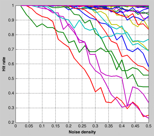
Figure 24.28 Noise test results of N-Tree model
Although the tests above show good performance for the hierarchical AM model on the ATT data set, we note that our model still fails to achieve the exact performance of the large single AM model (ARENA's direct implementation). In order to test our performance on a larger and more challenging problem, we used a second data set from The Facial Recognition Technology (FERET) Database [30]. The test subset we used has 2015 grayscale images of human faces from 724 people. For this data set, each subject has a different number of images, which range from 1 to 20. These images also include various facial expressions.
For the second set of tests, we use the same technique and same system specification as the ATT data set tests. That is, for each person, pick one image for testing and the rest for training. This gives 1291 images in the training data set and 724 images in the test data set. However, among these 724 subjects, the training set may have very few or even no images for some people. For example, if there is only one image for a person, this image will be used as test data and never be recognized correctly because the cluster analysis will have no instances of the person to train with. Hence, the recognition task on this data set is more difficult than that of the ATT data set due to it having more classes, unbalanced training data, and images with diverse features.
The results are presented in Figure 24.29, which indicates that hit rates of both the single flat AM model and the N-Tree decreased when compared to the ATT data set. Further, for this test data, the N-Tree model performs much worse than the single AM model with hit rates of only 29–51%.
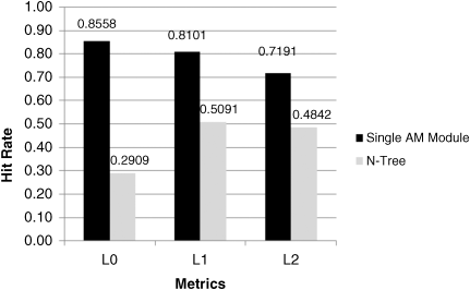
Figure 24.29 Retrieval performances on FERET data set
24.3.3 Fan-out versus Performance
Since our goal is to obtain the same retrieval performance as a single flat AM, we explore the correlation between the clustering tree's fan-out and performance. The fan-out of the N-Tree model is the size of each AM node. For example, if the fan-out is four, each data cluster splits into four subclusters during hierarchical k-means clustering, and each AM node can only store four subcluster centroids or image vectors. For a tree of a data set generated from hierarchical k-means clustering, fewer children for each node usually means smaller clusters, which may increase the possibility of making a mistake during the retrieval procedure. This is because once an AM unit outputs the “closest” centroid of a subcluster, the input pattern is compared with data in this subcluster only and may miss the real closest patterns. However, a larger cluster means more comparison operations and lower speed, to give a higher possibility of finding the right answer. We repeat the same simulation on the FERET data set but vary the fan-out number from 2 to 30. The results are all plotted in Figure 24.30. As we expect, generally a higher fan-out number improves the hit rate to some extent. However, it is still far worse than our goal.
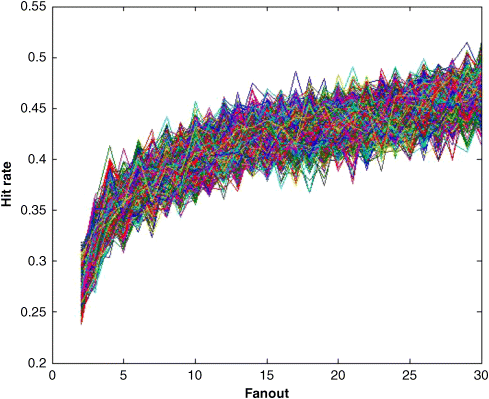
Figure 24.30 Fan-out versus hit rate for N-Tree model
24.3.4 Branch and Bound Search
The simulation results above tell us that the clustered data structure generated from the hierarchical k-means algorithm cannot provide us the same performance as the flat single AM model. The reason is that the hierarchical k-means clustering is initialized randomly and might not always cluster all the data to its nearest neighbor centroid.
To improve the performance of the hierarchical architecture, we adopt an algorithm called branch and bound search [31]. The basic idea is to search additional nodes that possibly contain a better answer, after we finish a routine N-Tree search. In other words, when a leaf node is visited at the end of the walk down of the tree using associative processing, we backtrack on the tree and check other nodes. The branch and bound search algorithm provides a method for generating a list of other nodes that need to be searched in order to optimize the result.
In branch and bound search, a simple rule can be used to check if a node contains a possible candidate for the nearest neighbor to the input vector. For a cluster with centroid Ci, we define its radius ri as the farthest distance between the centroid and any element in the cluster. Here we define X as the input vector and B as the distance between X and the best nearest neighbor found so far. Thus, if a cluster satisfies the condition:
where d is the distance function, then no element in cluster Ci can be nearer to X than the current bound B. Initially, B is set to be +∞. The distance function d gives the distance between two vectors as defined by a norm, for example, L0, L1, or L2. This rule is illustrated in Figure 24.31.
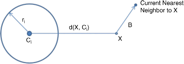
Figure 24.31 Branch and bound search rule
The full branch and bound search algorithm can be summarized as:
- Set B = +∞, current level L = 1, and current node to be root node.
- Place all child nodes of root node into the active list.
- For each node in the active list at the current level, if it satisfies the check rule, remove it from the active list.
- If the active list at the current level is empty, backtrack to the previous level, set L = L − 1, terminate the algorithm if L = 0, go to (2) if L is not 0. If there is a node in the list, go to (5).
- In the active list at the current level, choose the node that has the centroid nearest to input vector and call it the current node. If the current level is the final level, go to (6). Otherwise set L = L + 1, go to (1).
- In the final level, choose the stored vector which is nearest to the input vector X, and update B. Back track to previous level, set L = L − 1, go to (2).
Theoretically, branch and bound search can be guaranteed to find the nearest neighbor of an input vector from a hierarchical k-means clustered data set, which means it should have the same recognition performance as the flat single AM model.
Therefore, we enhance the N-Tree AM search with the branch and bound search algorithm and repeat the face recognition task. With the same training model, we see that branch and bound search always achieves the same performance as the ARENA algorithm, regardless of data set and fan-out for the N-Tree model. Figure 24.32 compares the hit rates of the flat (ARENA) model, the pure N-Tree model, and the branch and bound algorithms when the fan-out is four. The results indicate that the N-Tree model with branch and bound search can achieve the same performance of the ideal single AM module.
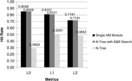
Figure 24.32 Retrieval performances on FERET data set
Table 24.1 gives us the number of nodes visited for the branch and bound search and indicates the efficiency of this technique compared to the simple N-Tree search with the L1 norm. However, the price of higher performance is lower efficiency. Without branch and bound search, the number of nodes visited is always just the depth of N-Tree structure, on average 9.3. To test all the possible candidates for nearest neighbor, the algorithm has to access additional nodes in the tree, on average 159.9, with a standard deviation of 86.2. This extra work is what is required to achieve the comparable performance of the flat network shown in Figure 24.32. Thus, there is an obvious tradeoff between hit rate and processing speed. The original search routine for the N-Tree model is “depth-only” one-way from the root node to a leaf node. In other words, if one AM unit in the middle level makes a wrong decision due to an imprecise clustered data set, the final output vector will be incorrect. In contrast, the branch and bound search provides opportunities to backtrack and search more possible clusters in other AM units at the cost of total search speed. As Table 24.1 shows, the average number of nodes that branch and bound search visits is 17 times as many as the original search of N-Tree model.
Table 24.1 Nodes visited in branch and bound search
| B&B search | Total nodes | Visited nodes | Visited leaf nodes |
| Maximum | 1199 | 454 | 293 |
| Minimum | 795 | 9 | 1 |
| Mean | 956.7 | 159.9 | 59.6 |
| Standard deviation | 34.3 | 86.28 | 47.4 |
| Average N-Tree size | Total nodes | Depth | Leaf nodes |
| 956.7 | 9.3 | 846.7 |
To speed up the search, we adjust the branch and bound search by fixing the condition of the checking rule as follows:
where α is a factor used to reduce the effective radius of the clusters, and ranges from 0 to 1. For some clusters, most elements are far away from X, only very few of them are in the bound. These clusters rarely contain the nearest neighbor. However, by the previous rule, we have to search them to guarantee optimality. Reducing the cluster's radius can help us avoid these less likely clusters and access significantly fewer nodes in the process.
In a final test, we sweep the value of α from 1 to 0 and observe the trends of hit rates and number of nodes visited during the search. The result is shown in Figure 24.33. We notice that the slopes of the three curves are different. Nodes searched decreases as radius is reduced. But the hit rate stays the same until α gets to 0.4. Thus, by reducing the cluster radius to some extent, we can improve the efficiency of searching without significantly sacrificing the hit rate.
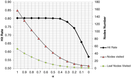
Figure 24.33 Performance versus speed of modified branch and bound search
24.4 Summary and Conclusion
24.4.1 Summary
In this chapter, we introduce the basic concept and brief history of associative memories both from the perspective of a pattern matching memory and in terms of their relationship to Oscillatory Neural Networks and develop a hierarchical associative memory for pattern matching.
We start by presenting the simulation of a hardware-based model of an Oscillatory Neural Network using phase-locked loops and simulate this model to show the functionality of these systems for pattern matching. We show that they perform this function by minimizing the energy of the system as they phase and frequency lock. We develop the design of an Associative Unit as a basic architectural building block and discuss several alternative emerging technology-based devices as candidates for efficient implementations of these blocks.
We then show a set of evolving designs for a hierarchical associative memory system. Our first hierarchical AM model is a simple system containing three levels of AM units. We then identify three problems with this simple design when compared to an ideal fully connected “flat” AM: Pattern Conflicts, Capacity Limits, and Representation Limits. To solve these problems we develop an improved version of the hierarchical model, which can solve the pattern conflict and representation limits but cannot solve the capacity limit problem.
We solve this final problem with a fundamentally different architecture: the N-Tree hierarchical model. For this model we change both the architecture and the recognition algorithm. We first show how the stored patterns are clustered and represented. Based on this data structure, we build a corresponding hierarchical tree structure from the same AM units. We test this architecture on two human face recognition problems. To further increase the recognition performance of the system, we add a branch and bound search algorithm which increases performance with little impact on search times.
24.4.2 Conclusion
Based on the design explorations in this chapter, we foresee several important research directions that can fundamentally change our notion of computing in the next decade.
First, we need to pursue both technologies and new computational functions at the same time, and not be tied to Boolean operations as the common building block of all computation. We see that for oscillatory neural networks, we can compute the DoM in an associative memory based on the attractor basins of the system's energy function. These can be formed by adjusting the coupling strength weights between oscillators or by using offsets on the frequency of the oscillators themselves. These networks can be implemented in one of several new technologies, including spin torque oscillators and resonant body transistor oscillators. Thus, associative pattern matching and retrieval operations can be done without using Boolean primitives.
Second, this is an opportunity to re-examine our notions of “memory” and “processing” as two distinct functions. Rather the incorporation of local processing together with storage might be a more promising avenue for the application of future nano-technologies. However, we need to address at the architectural level both the advantages and deficiencies of new technologies. We show that the scaling limitations of the oscillatory networks can be overcome by the use of hierarchy and partitioning.
Third, we must consider the application domain since we are not building general purpose processors. However, understanding the application can allow us to tailor the algorithms to more closely match the capabilities of the underling architecture. We show that the N-Tree model can realize an efficient associative memory for high dimension real number vectors and can approach the performance of an ideal model of nearest neighbor search. However, this is only possible because we first perform a clustering of the data. Thus, we partition the application into two phases – clustering and pattern retrieval – to optimize our use of the limited size of the AM modules.
Finally, we must be creative in our solutions. We see that the limitations on the size of the AM modules leads to a partitioning of the data that is less than ideal. Therefore, we add the use of a branch and bound search algorithm to improve the hit rate at the expense of multiple probes of the memory. This enlarges the search area and thus increases the possibility of finding the nearest pattern. Branch and bound search algorithms slow down the retrieval process but this tradeoff can be optimized by varying the search rules. Therefore, by moderately increasing the complexity of our algorithm, we can approach an optimum solution for our particular application.
Acknowledgments
The authors would like to thank the Intel University Research Office; George Bourianoff, Youssry Botros, and Dmitri Nikonov from Intel; Mircea Stan from the University of Virginia; Dan Hammerstrom from Portland State University; Dana Weinstein from MIT; Mathew Puffal and William Rippard from NIST; Tamas Roska from PPCU, Hungary; and Valeriu Beiu from UAEU, United Arab Emirates. This work was funded, in part, by the National Science Foundation under the grants INSPIRE “Track 1: Sensing and Computing with Oscillating Chemical Reactions,” DMR-1344178 and NSF “Expeditions in Computing Collaborative Research: Visual Cortex on Silicon,” CCF-1317373.
References
- 1. Lapique, L. (1907) Sur l'Excitation Electrique Des Nerfs. Journal of Physiology, 1907, 620–635.
- 2. Mead, C. (1989) Analog VLSI and Neural Systems, Addison-Wesley, Reading, MA.
- 3. McCulloch, W.S. and Pitts, W. (1943) A logical caculus of ideas immanet in nervous activity. Bulletin of Mathmatical Biophysics, 5, 59–62.
- 4. Hodgkin, A.L. and Huxley, A.F. (1952) Currents carried by sodium and potassium ions through the membrane of giant squid axon of loligo. Journal of Physiology, 116, 449–472.
- 5. Hawkins, J. and Dileep, G. (2006) Hierarchical Temporal Memory: Concepts, Theory and Terminology, Numenta Inc., www.numenta.com.
- 6. Riesenhuber, M. and Poggio, T. (1999) Hierarchical models of object recognition in cortex. Nature Neuroscience, 2, 1019–1025.
- 7. Hakin, S. (1999) Neural Networks: A Comprehensive Foundation, Prentice Hall, New Jersey.
- 8. Steinbuch, K. and Piske, U.A.W. (1963) Learning matrices and their applications. IEEE Transactions on Computers, EC-12, 846–862.
- 9. Willshaw, D.J., Buneman, O.P. et al. (1969) Non-holographic associative memory. Nature, 222, 960–962.
- 10. Buckingham, J. and Willshaw, D. (1992) Performance characteristics of the associative net. Network: Computation in Neural Systems, 3(4), 407–414.
- 11. Henson, R.N.A. and Willshaw, D. (1995) Short-term associative memory. Proceedings of the INNS World Congress on Neural Networks, 1, 438–441.
- 12. Anderson, J.A., Silverstein, J.W. et al. (1977) Distinctive features, categorical, perception, and probability learning: some applications of a neural model. Psychological Review, 84, 413–451.
- 13. Anderson, J.A. (1993) Associative Neural Memories: Theory and Implementation (ed. M.H. Hassoun), Oxford University Press.
- 14. Anderson, J.A., Allopenna, P. et al. (2007) Programming a Parallel Computer: The Ersatz Brain Project, in In Challenges for Computational Intelligence, Springer, Berlin Heidelberg, pp. 61–98.
- 15. Hopfield, J.J. (1982) Neural networks and physical systems with emergent collective computational abilities. Proceedings of the National Academy of Sciences, 79(8), 2554–2558.
- 16. Hoppensteadt, F.C. and Izhikevich, E.M. (1996) Synaptic organizations and dynamical properties of weakly connected neural oscillators: I. Analysis of canonical model. Biological Cybernetics, 75, 129–135.
- 17. Hoppensteadt, F.C. and Izhikevich, E.M. (2000) Pattern recognition via synchronization in phase-locked loop neural networks. IEEE Transactions on Neural Networks, 11, 734–738.
- 18. Shibata, T. (1993) Neuron MOS binary-logic integrated circuits: I. Design fundamentals and soft-hardware-logic circuit implementation. IEEE Transactions on Electron Devices, 40(3), 570–576.
- 19. Shibata, T., Zhang, R., Levitan, S.P. et al. (2012) CMOS supporting circuitries for nano-oscillator-based associative memories, 13th International Workshop on Cellular Nanoscale Networks and Their Applications (CNNA).
- 20. Tsoi, M. et al. (1998) Excitation of a magnetic multilayer by an electric current. Physical Review Letters, 80, 4281–4284.
- 21. Pufall, M.R., Rippard, W.H., Kaka, S. et al. (2005) Frequency modulation of spin-transfer oscillators. Applied Physics Letters, 86(8), 082506–082506-3.
- 22. Rippard, W.H., Pufall, M.R., Kaka, S. et al. (2005) Injection locking and phase control of spin transfer nano-oscillators. Physical Review Letters, 95(6), 067203.
- 23. Palm, G. (1980) On associative memory. Biological Cybernetics, 36, 19–31.
- 24. George, D. (2008) How the Brain Might Work: A Hierarchical and Temporal Model for Learning and Recognition, Electrical Engineering, Stanford University.
- 25. Levitan, S.P., Fang, Y., Dash, D.H. et al. (2012) Non-Boolean Associative Architectures Based on Nano-oscillators, 13th International Workshop on Cellular Nanoscale Networks and Their Applications (CNNA).
- 26. Duda, R.O., Hart, P.E., and Stork, D.G. (2000) Pattern Classification, John Wiley & Sons.
- 27. Cambridge University (2013) http://www.cl.cam.ac.uk/research/dtg/attarchive/facedatabase.html (accessed 16 July 2013).
- 28. Sim, T., Sukthankar, R., Mullin, M.D., and Baluja, S. (2000) High-Performance Memory-based Face Recognition for Visitor Identification, Proceedings of IEEE Conference on Automatic Face and Gesture Recognition, Grenoble, pp. 214–220.
- 29. Devijver, P.A. and Kittler, J. (1982) Pattern Recognition: A Statistical Approach, Prentice-Hall, London, GB.
- 30. NIST (2012) http://www.itl.nist.gov/iad/humanid/feret/feret_master.html (accessed 16 July 2013).
- 31. Fukunaga, K. (1975) A branch and bound algorithm for computing k-nearest neighbors. IEEE Transactions on Computers, C-24(7), 750–753.
