
CHAPTER 4
DV01, Duration, and Convexity
This chapter, along with Chapters 5 and 6, are about measuring and hedging interest rate risk. Market participants need to understand how fixed income prices change when interest rates change to take a view on the future level or term structure of interest rates, to ensure that a portfolio of assets keeps pace with a portfolio of liabilities, or to hedge one fixed income instrument or portfolio with another. But how exactly should a “change” in rates be defined? Chapters 1 through 3 show that pricing in fixed income markets can be expressed in terms of discount factors, par rates, spot rates, forward rates, yields, and spreads. Which of these quantities should be assumed to change and by how much?
In answering this question, there are two overarching trade‐offs: simplicity versus empirical reality, and robustness versus model dependence. With respect to the first trade‐off, a market maker who is hedging a long position in a 9.75‐year bond with a short position in a 10‐year bond over a short time period might reasonably rely on the simplest of frameworks, namely, that the yields of the two bonds will move up or down by the same number of basis points, that is, in parallel. A swap desk, by contrast, which is managing the risk of a portfolio of long and short swap positions of different terms, has to account for the reality that changes in rates across the term structure do not move perfectly in sync. With respect to robustness versus model dependence, a pension fund, which hedges the present value of its liabilities relative to the value of its assets, tends to prefer frameworks that are not very sensitive to assumptions about how rates of different terms vary relative to one another. An actively managed fixed income mutual fund, exchange‐traded fund, or hedge fund, by contrast, which is in the business of taking views on the level of rates and on the shape of the term structure, might gravitate toward frameworks designed to incorporate subjective views.
The one‐factor metrics and hedges described in this chapter are relatively simple along the lines just discussed, because they assume that rates of all terms move up and down together in some fixed relation. For example, if the 30‐year par rate changes by one basis point, it might be assumed that the 10‐year par rate changes by 0.99 basis points, in the same direction, while the five‐year rate changes by 0.8 basis points, in the same direction. The parallel‐shift assumption for bond yields is another simple framework described in this chapter.
The first several sections of this chapter introduce the metrics most often used to describe interest rate risk, namely, DV01, duration, and convexity, and illustrate these metrics by showing how to hedge Norfolk Southern Company's 100‐year or century bond with a shorter‐maturity Treasury bond. The next sections specialize the discussion to yield‐based versions of these metrics, which, while more restrictive in terms of their underlying assumptions, are very intuitive and widely used in practice. The final section presents a stylized case of asset–liability management at a pension fund, which requires choosing between barbell and bullet asset portfolios. Chapters 5 and 6 continue the discussion of risk metrics and hedges with multi‐factor and explicitly empirical approaches, respectively.
4.1 PRICE–RATE CURVES
The three bonds in Table 4.1 are used in this and subsequent sections to illustrate concepts. First, the Norfolk Southern Company (NSC) issued $600 million of the 4.10s of 05/15/2121 in May 2021 with a maturity of 100 years. Sales of century bonds are rare, but, with rates at historically low levels, bonds with very long maturities are being issued more often. The second and third bonds are the US Treasury 1.625s of 05/15/2026, issued in May 2016 with a bit less than $70 billion outstanding, and the 1.625s of 11/15/2050, issued in May 2020 with about $86 billion outstanding. The yields of these three bonds as of mid‐May 2021 are given in the table, along with their spreads to the High‐Quality Market‐Weighted (HQM) corporate bond yield curve. The HQM curve, published by the US Treasury, is designed to be representative of corporate bonds rated A or above and is intended for use by pension funds in computing the present value of their liabilities.
As discussed in the introduction, a “change” in rates has to be defined in order to compute interest rate risk metrics. For current purposes, the following assumptions are made. First, the base curve is the HQM par rate curve. Second, the spreads of the NSC and US Treasury bonds relative to the HQM curve, as listed in Table 4.1, do not change as the HQM curve changes. Third, the change in the HQM par rate of any term is a fixed proportion of the change in the 30‐year par rate. For example, if the 30‐year par rate moves up by one basis point, the 10‐year rate moves up by 0.99 basis points; the five‐year rate by 0.80 basis points; the two‐year rate by 0.37 basis points. These proportions are meant to capture the broad empirical fact, discussed further in Chapter 6, that short‐term rates are less volatile than long‐term rates. Figure 4.1 graphs the assumed shifts to the HQM par curve, which, for visibility, are scaled to a change of plus or minus 50‐basis points in the 30‐year par rate. It can easily be seen that, as intended, short‐term rates move by less than long‐term rates, and that the shift is close to a parallel shift for terms greater than 10 years.
TABLE 4.1 Selected Bonds with Indicative Levels as of Mid‐May 2021. Spreads Are Versus Par Rates from the High‐Quality Market‐Weighted Corporate Bond Curve, as of May 2021. Coupons and Yields Are in Percent. Spreads Are in Basis Points.
| Issuer | Coupon | Maturity | Yield | Spread |
|---|---|---|---|---|
| Norfolk Southern Company | 4.10 | 05/15/2121 | 4.103 | 66 |
| US Treasury | 1.625 | 05/15/2026 | 0.823 | −41 |
| US Treasury | 1.625 | 11/15/2050 | 2.363 | −97 |
Equipped with these assumptions, the prices of the bonds in Table 4.1 can be computed after the 30‐year HQM par rate changes by, say, one basis point. More specifically: i) given the one‐basis‐point change in the 30‐year par rate, calculate the change in par rates of all other terms along the lines of the previous paragraph; ii) for each bond, add its spread to the shifted par rates; iii) for each bond, convert the shifted par plus spread curve into discount factors; and iv) reprice each bond.
Figure 4.2 shows the results of these calculations. The horizontal axis gives changes in the 30‐year HQM par rate, and the vertical axis gives corresponding bond prices. Note that each rate change is assumed to be instantaneous; that is, no time passes as the rate changes from its current to its new level. In any case, as expected, prices increase as rates fall and decrease as rates rise. But the figure also shows that the three bonds do not have the same sensitivity to changes in rates. The price of the Treasury 1.625s of 05/15/2026, which has five years remaining to maturity, declines relatively mildly as rates increase; that is, its price is least sensitive to changes in rates. By the same token, the price of the Treasury 1.625s of 11/15/2050, which matures in 29.5 years, is more sensitive to rates, and the NSC century bond is the most sensitive of all. These differences in price sensitivities are quantified in the next sections as differences in DV01 or duration. Finally, the figure shows that the five‐year Treasury price–rate curve is not far from a line, whereas the price–rate curve of the 29.5‐year Treasury, and even more so of the NSC century bond, have noticeable curvature. These differences are quantified in subsequent sections as differences in convexity.
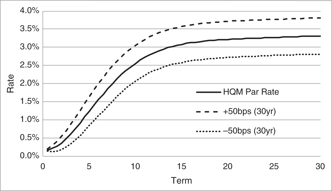
FIGURE 4.1 Sample Shifts to HQM Par Rates.
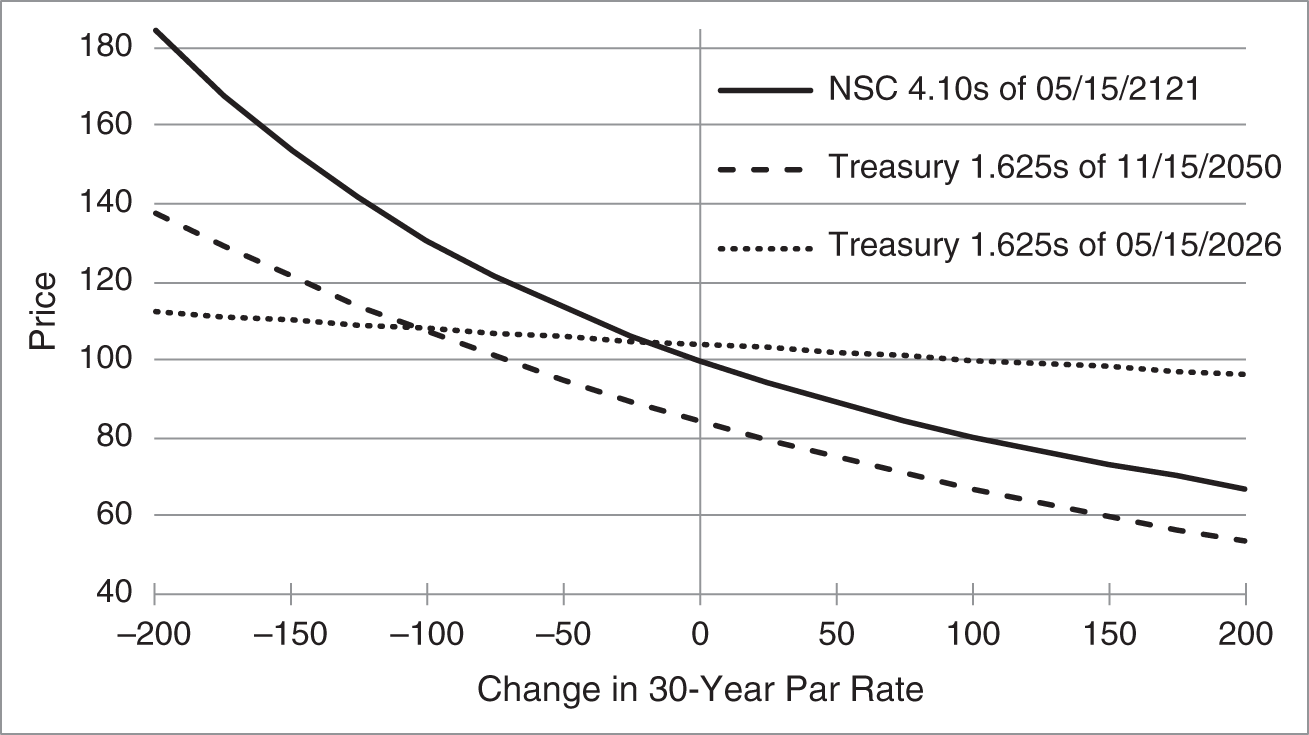
FIGURE 4.2 Price–Rate Curves for the Bonds in Table 4.1, as of Mid‐May 2021.
4.2 DV01
DV01 is an acronym for the dollar value of an '01, that is, the change in the price of a bond for a change in rates of 0.01%, or one basis point. As described in this section, DV01 can be applied in the context of any one‐factor model of changes in rates across the term structure. Practitioners typically use the term DV01, however, to mean yield‐based DV01, which is a narrower concept described in Section 4.7.
Table 4.2 illustrates the calculation of DV01 for the three bonds introduced in Table 4.1. Three prices are given for each bond. The price in column three is as of the pricing date in mid‐May 2021. The prices in columns two and four are the prices after a change in the 30‐year HQM par rate of ![]() or
or ![]() basis point, respectively. All other par rates fall or rise as well, of course, as discussed in the previous section. Given these prices, the first step in computing DV01 is to compute the slope of the price–rate curve, that is, the change in price divided by the change in rate. For the NSC 4.10s of 05/15/2021, the slope around the current market level is,
basis point, respectively. All other par rates fall or rise as well, of course, as discussed in the previous section. Given these prices, the first step in computing DV01 is to compute the slope of the price–rate curve, that is, the change in price divided by the change in rate. For the NSC 4.10s of 05/15/2021, the slope around the current market level is,
TABLE 4.2 Calculating DV01 for Bonds in Table 4.1, as of Mid‐May 2021.
| Bond | Price | Price | Price | Slope | DV01 |
|---|---|---|---|---|---|
| −1bp | +1bp | ||||
| NSC of May 2121 | 100.1801 | 99.9390 | 99.6990 | −2,406 | 0.241 |
| Treasury of May 2026 | 103.9621 | 103.9219 | 103.8817 | −402 | 0.040 |
| Treasury of Nov. 2050 | 84.5899 | 84.3906 | 84.1919 | −1,990 | 0.199 |
The left‐hand side of (4.1) is the difference between the bond prices at ![]() and
and ![]() basis point divided by the change in rates of
basis point divided by the change in rates of ![]() basis points, or 0.02%. Note that the current price – corresponding to a shift of 0 basis points – is not used in this calculation. From a numerical perspective, it is more accurate to estimate the slope of the curve at the current rate with shifts of
basis points, or 0.02%. Note that the current price – corresponding to a shift of 0 basis points – is not used in this calculation. From a numerical perspective, it is more accurate to estimate the slope of the curve at the current rate with shifts of ![]() and
and ![]() basis point, which are centered around the current rate, rather than with shifts of
basis point, which are centered around the current rate, rather than with shifts of ![]() and 0 basis points, which are centered slightly below the current rate, or with shifts of 0 and
and 0 basis points, which are centered slightly below the current rate, or with shifts of 0 and ![]() basis point, which are centered slightly above the current rate.
basis point, which are centered slightly above the current rate.
While Equation (4.1) gives ![]() 2,406 as the slope of the price–rate curve, its scale – the change in price per unit change in rates, that is, a change of 1.0 or 100% or 10,000 basis points – is not very intuitive. Much more intuitive and useful is the change in price for a one‐basis‐point change in rates. To this end, the slope can be divided by 10,000 to give, rounded to three decimal places,
2,406 as the slope of the price–rate curve, its scale – the change in price per unit change in rates, that is, a change of 1.0 or 100% or 10,000 basis points – is not very intuitive. Much more intuitive and useful is the change in price for a one‐basis‐point change in rates. To this end, the slope can be divided by 10,000 to give, rounded to three decimal places, ![]() 0.241. Furthermore, because the prices of almost all fixed income products fall as rates increase, it is conventional to drop the minus sign as understood. These two adjustments to the slope calculated in Equation (4.1) give the bond's DV01,
0.241. Furthermore, because the prices of almost all fixed income products fall as rates increase, it is conventional to drop the minus sign as understood. These two adjustments to the slope calculated in Equation (4.1) give the bond's DV01,
In words, a DV01 of 0.241 means that 100 face amount of the bond increases in price by 0.241 dollars or 24.1 cents when rates decrease by one basis point. Note that DV01 measures a price change per 100 face amount because the prices in Table 4.2 are per 100 face amount. While DV01, like price, is typically quoted per 100 face amount, it is occasionally useful to quote the DV01 of particular position. In these situations, DV01 is explicitly quoted in units of currency. For example, because the DV01 of the NSC century bond is 0.241 per 100 face amount, a position of $10 million has a DV01 of,
To generalize the discussion here, let ![]() denote the price of a fixed income instrument and let
denote the price of a fixed income instrument and let ![]() denote the single factor that determines rate changes across the term structure, which, in the context of this chapter, is the 30‐year HQM par rate. Finally, let
denote the single factor that determines rate changes across the term structure, which, in the context of this chapter, is the 30‐year HQM par rate. Finally, let ![]() denote the change in the factor
denote the change in the factor ![]() and
and ![]() the change in the price given that change in
the change in the price given that change in ![]() . With this notation, the DV01 of a fixed income instrument is estimated by,
. With this notation, the DV01 of a fixed income instrument is estimated by,
The slope of the NSC bond's price–rate curve at the current rate is estimated in Equations (4.1) and (4.2) with prices at levels one basis point below and one basis point above the current rate. A more accurate estimate might be obtained by shifting the current rate up and down by 0.5 basis points, or 0.1 basis points, etc. In the calculus, the limit of the resulting estimates of the slope, as the size of the shift shrinks to zero, is known as the derivative and denoted ![]() . In some cases, like the yield‐based metrics discussed later in this chapter, the derivative of the price–rate function can be written in closed form, that is, with a relatively simple mathematical formula. More generally, however, prices and the slope of the price–rate function have to be calculated numerically. In any case, the limit of Equation (4.4) as the size of the shift shrinks to zero gives DV01 in terms of the derivative instead of the slope,
. In some cases, like the yield‐based metrics discussed later in this chapter, the derivative of the price–rate function can be written in closed form, that is, with a relatively simple mathematical formula. More generally, however, prices and the slope of the price–rate function have to be calculated numerically. In any case, the limit of Equation (4.4) as the size of the shift shrinks to zero gives DV01 in terms of the derivative instead of the slope,
The derivative of a curve at a particular point is often illustrated with tangent lines. In Figure 4.3, the solid black line is the price–rate curve of the NSC century bonds, which is also shown in Figure 4.2. The dashed line is the tangent line of the curve at the current market rate. This means that the slope of the line equals the derivative of the curve at the current market rate, and that the line just touches the curve at that rate. Figure 4.3 also shows the tangent line to the curve at a rate 150 basis points below the current market rate. The slope of this tangent line is clearly steeper than the other, which means that the NSC 4.10s of 05/15/2121 are more sensitive to rates at 150 basis points below the current rate than they are at the current rate.
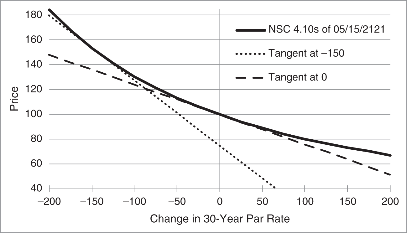
FIGURE 4.3 Tangent Lines to the Price–Rate Curve of the NSC 4.10s of 05/15/2121, as of Mid‐May 2021.
DV01 is said to be a local measure of interest rate sensitivity because the slope of the price–rate curve, and, therefore, DV01, change as rate changes. This property of price–rate curves is known as convexity and is introduced later in the chapter.
This section concludes by noting that the DV01 of a portfolio of fixed income instruments is equal to the sum of the DV01s of its component instruments. A portfolio with 100 face amount of the NSC bonds – with a DV01 of 0.241 – and 500 face amount of the Treasury 1.625s of 05/15/2026 – with a DV01 of ![]() – has a total DV01 of
– has a total DV01 of ![]() , or 0.441. This very intuitive rule is proved formally in Appendix A4.1.
, or 0.441. This very intuitive rule is proved formally in Appendix A4.1.
4.3 HEDGING A CENTURY BOND: PART I
Say that a market maker buys from a client $10,000,000 face amount of the NSC 4.10s of 05/15/2121 at the going bid price. The market maker does not turn around and immediately sell those bonds at market, because that would likely mean selling at the same bid price, leaving no overall profit from the trades. Instead, the market maker waits until other clients appear, who are willing to pay the higher ask price. In this way, the market maker earns the bid–ask spread for providing immediacy or liquidity both to the client who originally sells the bonds and to the clients who later buy the bonds.
This strategy, however, exposes the market maker to the risk that the price of the corporate bond falls before it can be sold. The typical solution is to hedge that risk by selling a liquid Treasury bond when buying the corporate, and then buying back that Treasury bond when selling the corporate. Because a liquid Treasury bond, by definition, has a very narrow bid–ask spread, this strategy protects the market maker against falling prices at the cost of that narrow bid–ask spread, which leaves much of the wider, corporate bid–ask spread as profit.
The next question, therefore, is which Treasury bond to sell. Because, as mentioned earlier, rates of different terms can behave differently, a reasonable choice is to sell a Treasury bond with about the same maturity as the corporate bond being hedged. In the particular situation at hand, however, there is no Treasury bond with a maturity anywhere near 100 years. The best the market maker can do, therefore, is to sell one of the longest maturity Treasuries outstanding, like the 1.625s of 11/15/2050.
The final question, then, is what face amount of Treasury bonds to sell against the purchase of $10 million face amount of the NSC bonds. One common solution is to ensure that the net DV01 of the combined position is zero. In other words, choose the face amount of Treasuries such that, if rates change by one basis point, the value of the net position is unchanged. Denoting the face amount of the Treasury hedge by ![]() , and using the DV01s of the two bonds computed in Table 4.2,
, and using the DV01s of the two bonds computed in Table 4.2, ![]() is determined by the following equation,
is determined by the following equation,
The first term of (4.6) gives the change in the value of ![]() face amount of Treasury bonds if rates fall by one basis point – 19.9 cents per 100 face amount, and, therefore,
face amount of Treasury bonds if rates fall by one basis point – 19.9 cents per 100 face amount, and, therefore, ![]() times 0.199/100 for
times 0.199/100 for ![]() face amount. The second term, along the same lines, gives the change in the value of the
face amount. The second term, along the same lines, gives the change in the value of the ![]() million face amount of NSC bonds if rates fall by one basis point. The equation as a whole, therefore, requires that the combined, hedged position neither gains nor loses value when rates fall by one basis point. And because the hedged profit and loss (P&L) when rates fall by some other number of basis points is just that number of basis points times the left‐hand side of (4.6), the equation holds for that number of basis points as well (subject, of course, to the limitation of DV01 as a local measure of interest rate sensitivity).
million face amount of NSC bonds if rates fall by one basis point. The equation as a whole, therefore, requires that the combined, hedged position neither gains nor loses value when rates fall by one basis point. And because the hedged profit and loss (P&L) when rates fall by some other number of basis points is just that number of basis points times the left‐hand side of (4.6), the equation holds for that number of basis points as well (subject, of course, to the limitation of DV01 as a local measure of interest rate sensitivity).
Solving Equation (4.6) for ![]() ,
,
Hence, the market maker can hedge its $10 million face amount of the NSC bonds by selling about $12.1 million face amount of the Treasury bond. Intuitively, because the price of the NSC bonds changes by 24.1 cents per 100 face amount per basis point, while the Treasury bonds change by only 19.9 cents, the market maker has to sell a larger face amount of Treasuries than it buys of NSC bonds to achieve a DV01‐neutral position.
To elaborate on how the hedge works, say that rates rise by five basis points after the market maker established the position. The NSC bonds fall in value, losing approximately ![]() . At the same time, the Treasury bonds also fall in value, gaining – because the market maker is short – approximately
. At the same time, the Treasury bonds also fall in value, gaining – because the market maker is short – approximately ![]() . Hence, as intended, the overall, hedged position does not gain or lose money.
. Hence, as intended, the overall, hedged position does not gain or lose money.
In general, if the DV01s of bonds A and B are ![]() and
and ![]() , then
, then ![]() face amount of bond A is hedged with
face amount of bond A is hedged with ![]() face amount of bond B such that,
face amount of bond B such that,
Equation (4.8) is the generalization of Equation (4.6). The general solution, Equation (4.9), reveals two intuitive points about DV01 hedging. First, a long position in bond A is hedged by a short position in bond B. Second, the bond with the higher DV01 is traded in smaller quantity. In the market making example, a long position in the NSC bonds is hedged by a short position in Treasury bonds, and, because the DV01 of the NSC bonds is greater than that of the Treasury bonds, $10 million of NSC bonds is hedged by $12.1 million of Treasury bonds.
The section concludes with a reminder of the assumptions behind the DV01 hedge constructed here. First, rate shifts across terms are assumed to be proportional to those illustrated in Figure 4.1. If it turns out that the 100‐year and 29.5‐year par rates move differently than as assumed, the hedge will not work as intended. To the extent that this is a concern, the hedges described in Chapters 5 and 6 might be more appropriate. Second, the spreads of the NSC and Treasury bonds to the base curve are assumed to be constant. If it turns out that these spreads behave differently, then, again, the hedge will not work as intended. This concern is not as easily addressed. A safer hedge would be to sell a corporate bond, whose spread is more highly correlated with the NSC bond spread than is the Treasury bond spread. But hedging with a relatively illiquid corporate bond instead of an extremely liquid Treasury bond is likely to wipe out any market making P&L. Therefore, bearing spread risk for short periods of time may be an integral part of corporate bond market making and, in turn, may enter into the determination of bid–ask spreads in that market.
4.4 DURATION
Another popular metric for interest rate sensitivity is duration. Whereas DV01 measures the change in price for a change in rates, duration measures the percentage change in price for a change in rates. Like DV01, duration can be defined in any one‐factor framework, but practitioners often use the term duration to mean yield‐based duration (described in Section 4.7) and use the term effective duration to mean the more general case presented here.
Using the same notation as in Section 4.2, duration, ![]() , is estimated in terms of the slope as,
, is estimated in terms of the slope as,
and given in terms of the derivative as,
Because ![]() and
and ![]() both represent percentage change in price, Equations (4.10) and (4.11) express duration as the percentage change in price for a change in rates. Also, for intuition, it is useful to rewrite Equation (4.10) as,
both represent percentage change in price, Equations (4.10) and (4.11) express duration as the percentage change in price for a change in rates. Also, for intuition, it is useful to rewrite Equation (4.10) as,
Table 4.3 shows the calculation of duration for the three bonds introduced in Table 4.1. Estimating the duration of the NSC 4.10s of 05/15/2121 with Equation (4.10),
Applying Equation (4.12), the percentage change in the price of the NSC bond for a decline in rates of 100 basis points, or 1%, is ![]() . Hence, a duration of 24.1 roughly means that a fall in rates of 100 basis points increases bond price by 24.1%. This interpretation is only roughly correct because duration, like DV01, is based on the slope of the price–rate curve and, therefore, is a local measure of price change.
. Hence, a duration of 24.1 roughly means that a fall in rates of 100 basis points increases bond price by 24.1%. This interpretation is only roughly correct because duration, like DV01, is based on the slope of the price–rate curve and, therefore, is a local measure of price change.
TABLE 4.3 Calculating Duration for Bonds in Table 4.1, as of Mid‐May 2021.
| Bond | Price | Price | Price | Slope | Duration |
|---|---|---|---|---|---|
| −1bp | +1bp | ||||
| NSC of May 2121 | 100.1801 | 99.9390 | 99.6990 | −2,405.5 | 24.1 |
| Treasury of May 2026 | 103.9621 | 103.9219 | 103.8817 | −402.00 | 3.9 |
| Treasury of Nov. 2050 | 84.5899 | 84.3906 | 84.1919 | −1,990 | 23.6 |
While traders tend to rely on DV01, asset managers tend to rely on duration. As in the market‐making example of the previous section, traders typically want to ensure that the dollar changes in the value of long and short positions offset each other. Also, because the sizes of their positions can fluctuate rapidly, and because they typically borrow money to buy bonds, they tend to focus on dollar P&L rather than on returns on fixed amounts of invested cash. Asset managers, in contrast, typically invest a slowly changing pool of funds and focus on rates of return. Looking at the durations in Table 4.3, an asset manager immediately sees that the NSC bond has the most interest rate risk, in that an investment in that bond loses 2.41% for a 10‐basis point increase in rates. An investment in the Treasury 1.625s of 11/15/2050 has slightly less risk, losing 2.36% for that 10‐basis‐point increase in rates, while an investment in the Treasury 1.625s of 05/15/2026 has the least risk, losing only 0.39% in that scenario. The asset manager can weigh these risks against expected returns and other factors in making a final investment decision.
This section concludes by noting the duration of a portfolio is equal to the weighted sum of the durations of its component holdings, where the weights are percentages of portfolio value. For example, the duration of a portfolio with 25% of its value in the NSC bonds – with a duration of 24.1 – and 75% of its value in the Treasury 1.625s of 05/15/2026 – with a duration of 3.9 – is ![]() . The DV01 of a portfolio is the sum of its component DV01s, while the duration of a portfolio is the value‐weighted sum of its component durations, because DV01 represents a change in price, while duration represents a percentage change in price. A formal proof is in Appendix A4.1.
. The DV01 of a portfolio is the sum of its component DV01s, while the duration of a portfolio is the value‐weighted sum of its component durations, because DV01 represents a change in price, while duration represents a percentage change in price. A formal proof is in Appendix A4.1.
4.5 CONVEXITY
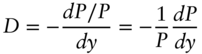
As can be seen from the tangent lines in Figure 4.3, the interest rate sensitivity of a bond falls as rates increase. Making this point more directly, Figure 4.4 graphs the DV01 of the Treasury 1.625s of 11/15/2050, a 29.5‐year bond, and of the Treasury 1.625s of 05/15/2026, a five‐year bond. DV01 falls as rates increase, but the rate of decline is much faster for the 29.5‐year bond than for the five‐year bond.
A curve is said to have a convex shape if a line connecting two points on that curve lies above the curve. The price–rate curves of coupon bonds are convex, and Figure 4.3 makes it clear that the convex shape of the price–rate curve is tantamount to DV01 falling as rates increase. For this reason, the relationship between DV01 and the level of rates is called convexity. The property of DV01 falling as rates increase is called positive convexity, while the property of DV01 rising as rates increase is called negative convexity.
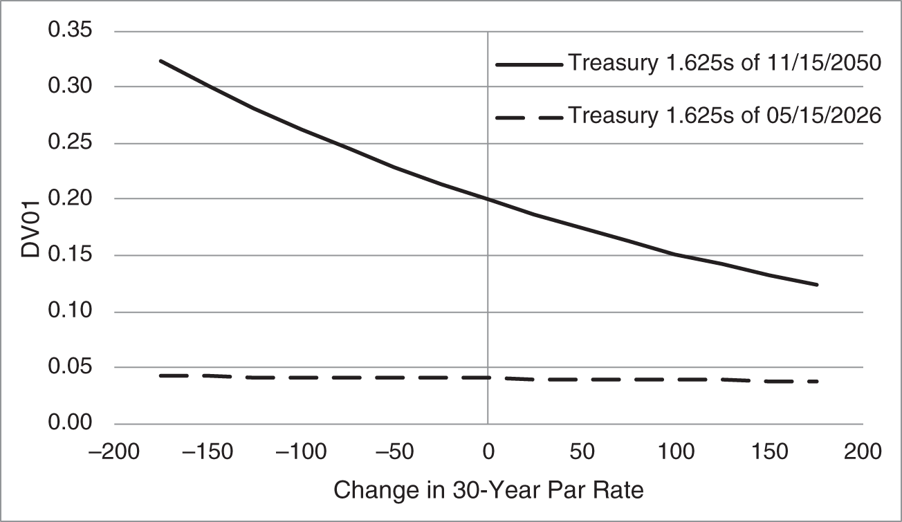
FIGURE 4.4 DV01s of the Treasury 1.625s of 11/15/2050 and of the Treasury 1.625s of 05/15/2026, as of Mid‐May 2021.
Mathematically, convexity, ![]() , is defined as,
, is defined as,
the second derivative of the price–rate function divided by price. To summarize, all of these statements are equivalent: the price–rate curve is convex; its second derivative is positive; its first derivative becomes less negative as rates increase; and its DV01 falls as rates increase.
Table 4.4 calculates the convexity of the NSC bond and of the two Treasury bonds as of mid‐May 2021. For each bond, three prices are given: the current market price, the price after the 30‐year par rate falls by one basis point, and the price after the 30‐year par rate rises by one basis point. Then, two first derivatives, or slopes, are computed for each bond. These slopes are computed just as in Equation (4.1), but the slopes here are centered around the 30‐year par rate plus and minus 0.5 basis points.
The final step in Table 4.4 is to estimate the convexity as defined in Equation (4.14). The second derivative centered at the current rate (i.e., a “change” of 0.0) is estimated as the change in the first derivatives from +0.5 to ![]() 0.5 basis points divided by the change in rates of
0.5 basis points divided by the change in rates of ![]() , or 1 basis point. Dividing the result by price gives the estimate of convexity centered at current market levels. For the NSC bond,
, or 1 basis point. Dividing the result by price gives the estimate of convexity centered at current market levels. For the NSC bond,
As expected from the curvatures of the price–rate curves in Figure 4.2, the convexity measure is largest for the NSC century bond, smaller for the 29.5‐year Treasury bond, and yet smaller for the five‐year Treasury bond.
TABLE 4.4 Calculating Convexity for Bonds in Table 4.1, as of Mid‐May 2021. Rate Changes Are in Basis Points.
| Rate Change | Price | 1st Derivative | Convexity |
|---|---|---|---|
| NSC 4.10s of 05/15/2121 | |||
| −1.0 | 100.180067 | ||
| −0.5 | −2,410.67 | ||
| 0.0 | 99.939000 | 1,101 | |
| 0.5 | −2,399.67 | ||
| 1.0 | 99.699033 | ||
| Treasury 1.625s of 11/15/2050 | |||
| −1.0 | 84.589932 | ||
| −0.5 | −1,993.08 | ||
| 0.0 | 84.390624 | 648 | |
| 0.5 | −1,987.61 | ||
| 1.0 | 84.191863 | ||
| Treasury 1.625s of 05/15/2026 | |||
| −1.0 | 103.962050 | ||
| −0.5 | −401.75 | ||
| 0.0 | 103.921875 | 12 | |
| 0.5 | −401.63 | ||
| 1.0 | 103.881712 | ||
Convexity values are not as easily interpreted as DV01 and duration values, but consider the following. Equation (4.12) showed that the percentage change in a bond's price approximately equals the negative of its duration times the change in rate. However, Appendix A4.2 shows that a better approximation uses both the bond's duration and convexity,
Because duration appears in the first term of (4.16) and convexity in the second, using duration alone is called a first‐order approximation, while using both duration and convexity is called a second‐order approximation.
Illustrating with the NSC bonds, which have a duration of 24.1 (Table 4.3) and a convexity of 1,101 (Table 4.4), estimates of the percentage change in price after rates fall by 100 basis points, or 1%, are,
using duration alone, and,
using both duration and convexity. The actual price of the bond after rates decline by 100 basis points is 130.898, which translates into a true percentage price change of ![]() , or 30.978%. Therefore, adding the convexity term in Equations (4.16) and (4.18) does result in a more accurate approximation.
, or 30.978%. Therefore, adding the convexity term in Equations (4.16) and (4.18) does result in a more accurate approximation.
Figure 4.5 makes the same point graphically. The actual price of the NSC bonds is given by the solid curve. The approximation to prices after various changes in rates using just duration or DV01 is given by the dashed line, which is the same dashed tangent shown in Figure 4.3. And the approximation using both duration and convexity is given by the dotted line. Because both duration and convexity are local estimates, using derivatives at current market levels to estimate prices, both the dashed and dotted lines are less and less accurate as rates move further from current levels. It is clear to the eye, however, that the approximation using both duration and convexity is relatively close to the true price for larger changes in rates than is the approximation using duration alone.
FIGURE 4.5 Price–Rate Curve of the NSC 4.10s of 05/15/2121, as of Mid‐May 2021, with Price Approximations Using Duration and Using both Duration and Convexity.
Returning now to interpreting convexity numbers, the difference between approximating percentage price change with both duration and convexity [Equation (4.18)] and with duration alone [Equation (4.17)] is the term,
Therefore, noting that ![]() equals one basis point, the correction of 5.5% in (4.19) is half the convexity divided by 10,000. In other words, for a 1% change in rates, the second‐order correction to the duration approximation of price change is half the convexity divided by 10,000 (i.e., 0.055), or equivalently, the percentage correction is half the convexity divided by 100 (i.e., 5.5).
equals one basis point, the correction of 5.5% in (4.19) is half the convexity divided by 10,000. In other words, for a 1% change in rates, the second‐order correction to the duration approximation of price change is half the convexity divided by 10,000 (i.e., 0.055), or equivalently, the percentage correction is half the convexity divided by 100 (i.e., 5.5).
The section concludes by noting that the convexity of a portfolio equals the weighted sum of the convexities of its component holdings, where the weights are percentages of portfolio value. The convexity of a portfolio with 25% of its value in the NSC bonds – with a convexity of 1,101 – and 75% of its value in the Treasury 1.625s of 05/15/2026 – with a convexity of 12 – is ![]() . Portfolio convexity is a weighted sum, as is portfolio duration, because both metrics divide by price: duration divides the change in price by price, and convexity divides the second derivative divided by price. A formal proof is given in Appendix A4.1.
. Portfolio convexity is a weighted sum, as is portfolio duration, because both metrics divide by price: duration divides the change in price by price, and convexity divides the second derivative divided by price. A formal proof is given in Appendix A4.1.
4.6 HEDGING A CENTURY BOND: PART II
Section 4.3 explained why and how a market maker hedges the DV01 from $10 million face amount of the NSC 4.10s of 05/15/2121 by selling $12.1 million face amount of the Treasury 1.625s of 11/15/2050. This section shows that this hedge leaves the market maker with a long convexity position and describes the resulting risk and P&L implications.
Figure 4.6 shows the P&L of $100 million face amount of the NSC century bond and of $121 million face amount of the 29.5‐year Treasury bond. For example, the prices of these bonds in mid‐May 2021 were 99.939 and 84.391, respectively, and if rates fell by 100 basis points, their prices would be 130.898 and 107.309, respectively. Hence, the P&L from $100 million of the one and $121 million of the other is $100 million × ![]() , or $30.96 million, and $121 million ×
, or $30.96 million, and $121 million × ![]() , or $27.7 million, respectively.
, or $27.7 million, respectively.
Section 4.3 showed that, with these face amounts, the two positions have the same DV01 at current market levels. Figure 4.6 reflects this fact in that the two P&L curves are tangent to each other, that is, they have the same slope, at current rates. Both bonds are positively convex, of course, but, because the NSC bonds are more convex (Table 4.4), their P&L exceeds the P&L on the Treasury bonds whether rates fall or rise. This result is emphasized by the dotted line in the figure, graphed against the right axis, which is the P&L of the NSC bonds minus the P&L of the Treasury bonds and which, in turn, is the net P&L of the market maker in this application. This net P&L is zero, of course, at current market levels but is positive for both negative and positive rate changes, and particularly large for large, negative changes.
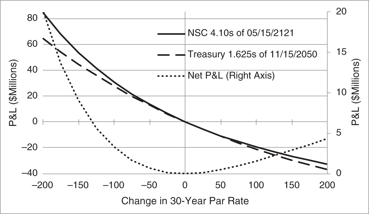
FIGURE 4.6 P&L of a Long Position of $100 Million Face Amount of the NSC 4.10s of 05/15/2121, a DV01‐Equivalent Long Position in the Treasury 1.625s of 11/15/2050, and a Position Long the NSC Bonds and Short the Treasury Bonds, as of Mid‐May 2021.
Expanding on the results of the previous paragraph, for unchanged rates and prices, the P&L of both bond holdings is clearly zero. If rates fall, both bonds increase in price and – because they are both positively convex – both their DV01s increase as well. But because the NSC bonds are more convex, their DV01 increases by more, which, for falling rates, means higher profits. Instead, if rates rise, both bonds decrease in price and in DV01. But because the NSC bonds are more convex, their DV01 falls by more, which, for rising rates, means lower losses. Therefore, whether rates fall or rise, the P&L on the NSC bonds exceeds the P&L on a DV01‐equivalent amount of Treasury bonds.
The market maker is said to have a positively convex position and to be long convexity because the convexity of its long position (NSC bonds) is greater than the convexity of its short position (Treasury bonds) and because its P&L seems to be positive whether rates fall or rise. But is it really the case that the market maker profits from the position no matter what? If so, why don't arbitrageurs initiate positions that are long the century NSC bonds and short the 29.5‐year Treasury bonds?
These questions can be answered by noting that Figure 4.6 omits an important variable: time. As mentioned earlier, all of the figures in this chapter assume an instantaneous change in rates, that is, with no passage of time. As it turns out, however, bonds or portfolios that are more convex tend to earn less over time. Therefore, the full story of a positively convex position, or of being long convexity, is that the position profits if rates move down or up by a sufficient amount. If rates change by less than that, or stay the same, the position loses money. In this sense, a long convexity position is also long volatility. In any case, this is a fundamental property of asset pricing, applicable to both stock options and coupon bonds. Section 4.8 explores the topic further in the context of pension asset–liability management, and Chapter 8 shows how convexity fits into a general framework of returns.
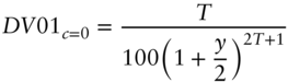
4.7 YIELD‐BASED DV01, DURATION, AND CONVEXITY
Previous sections described DV01, duration, and convexity in a general, one‐factor framework: specify the way changes in a rate or factor change the entire term structure, re‐price bonds after the change, and compute risk metrics. This section is about yield‐based metrics, for which a change in rates means a fixed change in bond yields. These metrics have two significant weaknesses. One, they are defined only for bonds with fixed cash flows, but not, for example, for a callable bond or a mortgage. Two, their use implicitly assumes parallel shifts in bond yields, which is not an empirically sound assumption. Nevertheless, there are several reasons to study and understand yield‐based metrics. First, they are simple to compute and easy to understand, and, in many situations, are perfectly reasonable to use. Second, these metrics are widely used across the financial industry. Third, much of the intuition gained from understanding these metrics carries over to more general frameworks.
The reason that yield‐based metrics are easy to compute is that price can be written as a function of yield, in the forms of Equations (3.7) and (3.8). Recalling that ![]() is the annual coupon payment and
is the annual coupon payment and ![]() is the number of years to maturity, these equations are repeated here for convenience,
is the number of years to maturity, these equations are repeated here for convenience,
With these expressions, DV01 and duration, as defined in Equations (4.5) and (4.11), can be solved explicitly. Calculate the derivative of the previous price‐yield relationships and then divide by ![]() 10,000 to find DV01 or by
10,000 to find DV01 or by ![]() to find duration. The resulting formulas for yield‐based DV01 are,
to find duration. The resulting formulas for yield‐based DV01 are,
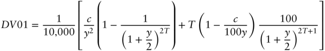
and for yield‐based duration are,
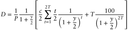
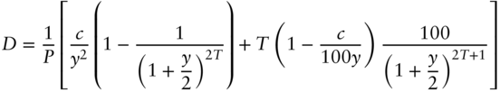
This formulation of yield‐based duration is also known in the industry as modified and adjusted duration.1
The terms inside the square brackets of Equations (4.22) and (4.24) have an intuitive interpretation that sheds light on these risk metrics. The terms ![]() and
and ![]() represent the times to receipt of each cash flow, that is, 0.5 years, 1 year, 1.5 years, and so forth, out to
represent the times to receipt of each cash flow, that is, 0.5 years, 1 year, 1.5 years, and so forth, out to ![]() years, the years to maturity. And each of these terms is multiplied by the present value of the cash flow to be received at that time, that is,
years, the years to maturity. And each of these terms is multiplied by the present value of the cash flow to be received at that time, that is, ![]() for the coupon payments and
for the coupon payments and ![]() for the principal payment. Putting this all together, the sum of the terms in brackets can be described as the weighted sum of the times at which cash flows are received, with each weight equal to the present value of the cash flow received at that time. Furthermore, in the case of duration, where the bond price can be moved inside the brackets, each weight can be described as the present value of the cash flow received at that time divided by the bond price, which is the sum of all the present values. Therefore, this weight is simply the proportion of the bond's value contributed by that cash flow.
for the principal payment. Putting this all together, the sum of the terms in brackets can be described as the weighted sum of the times at which cash flows are received, with each weight equal to the present value of the cash flow received at that time. Furthermore, in the case of duration, where the bond price can be moved inside the brackets, each weight can be described as the present value of the cash flow received at that time divided by the bond price, which is the sum of all the present values. Therefore, this weight is simply the proportion of the bond's value contributed by that cash flow.
Table 4.5 illustrates this interpretation by calculating the yield‐based DV01 and duration of the Treasury 1.625s of 05/15/2026 as of mid‐May 2021. The first column gives the term of each cash flow; the second column gives the cash flows; and the third column gives the present value of each cash flow discounted at 0.82277%, the bond's yield at the time. For example, the present value of the coupon payable in 2.5 years is,
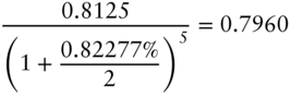
The sum of the present values of the cash flows is just the market price, in this case, 103.9219. The fourth column gives the present value of each cash flow as a percentage of the market price. Not surprisingly, for a bond maturing in five years and trading at a small premium, the principal accounts for a large share of the bond's value, in this case, over 93%.
TABLE 4.5 Calculating the Yield‐Based DV01 and Duration of the Treasury 1.625s of 05/15/2026 at a Yield of 0.82277%, as of Mid‐May 2021.
| (1) | (2) | (3) | (4) | (5) | (6) |
|---|---|---|---|---|---|
| Cash | Present | PV/Price | Term | Term‐Wtd | |
| Term | Flow | Value | (%) | PV/Price | PV |
| 0.5 | 0.8125 | 0.8092 | 0.779 | 0.0039 | 0.4046 |
| 1.0 | 0.8125 | 0.8059 | 0.775 | 0.0078 | 0.8059 |
| 1.5 | 0.8125 | 0.8026 | 0.772 | 0.0116 | 1.2038 |
| 2.0 | 0.8125 | 0.7993 | 0.769 | 0.0154 | 1.5985 |
| 2.5 | 0.8125 | 0.7960 | 0.766 | 0.0191 | 1.9900 |
| 3.0 | 0.8125 | 0.7927 | 0.763 | 0.0229 | 2.3782 |
| 3.5 | 0.8125 | 0.7895 | 0.760 | 0.0266 | 2.7632 |
| 4.0 | 0.8125 | 0.7862 | 0.757 | 0.0303 | 3.1450 |
| 4.5 | 0.8125 | 0.7830 | 0.753 | 0.0339 | 3.5236 |
| 5.0 | 100.8125 | 96.7575 | 93.106 | 4.6553 | 483.7877 |
| Sum | 103.9219 | 100.000 | 4.8267 | 501.6005 | |
| Duration: | 4.8069 | ||||
| DV01: | 0.0500 |
The fifth column of the table multiplies each present value proportion by its term: 0.5 weighted by 0.779%, 1.0 weighted by 0.775%, and so forth, and 5.0 weighted by 93.106%. In this way, the sum of the column is the weighted average of the payment times, with weights equal to the value proportion of each payment. In terms of Equation (4.24), this weighted average, 4.8267, is the sum of the terms in brackets divided by price. Duration, therefore, is ![]() , or 4.8069. This interpretation explains why many market participants say that this bond has a duration of 4.83 years: the value of the bond is paid, on average, in 4.83 years.2 This interpretation also explains why the duration of a coupon bond is somewhat less than its maturity: while most of a bond's value is paid at maturity, some portion is paid earlier.
, or 4.8069. This interpretation explains why many market participants say that this bond has a duration of 4.83 years: the value of the bond is paid, on average, in 4.83 years.2 This interpretation also explains why the duration of a coupon bond is somewhat less than its maturity: while most of a bond's value is paid at maturity, some portion is paid earlier.
Lastly, the sixth column of the table gives term times present value. The sum of this column is the sum of the terms in brackets in Equation (4.22), which means that DV01 is ![]() .
.
As mentioned earlier, the intuition derived from yield‐based measures is often useful for understanding more general risk metrics. A lot of this intuition arises from the relatively simple expressions for yield‐based DV01 and duration in Equations (4.23) and (4.25), and from the extremely simple expressions in the case of zero coupon bonds and par bonds. To derive these latter expressions, simply substitute ![]() and then
and then ![]() into the price equation, (4.21), and into the DV01 and duration equations just referenced, to obtain the following. For a zero coupon bond,
into the price equation, (4.21), and into the DV01 and duration equations just referenced, to obtain the following. For a zero coupon bond,
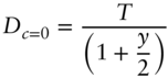
And for a par bond,
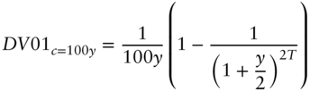
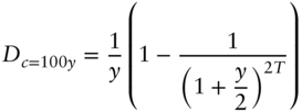
FIGURE 4.7 Yield‐Based Duration for Bonds with Coupons of 0%, 2%, and 5%. Yield Equals 2%.
The discussion now turns to using these simple expressions to understand how yield‐based duration and DV01 depend on a bond's maturity, coupon, and yield. Figure 4.7, fixing yield for all bonds at 2%, graphs the duration of bonds of terms out to 40 years with coupons of 0%, 2%, and 5%. Several lessons can be taken from this figure.
First, the duration of a zero coupon bond is approximately equal to its term, which can also be seen from Equation (4.28). Second, the duration of a par bond, in this case, of all bonds with a coupon of 2%, increases with term, which can also be deduced from Equation (4.30).3 In addition, however, the figure illustrates how the duration of par bonds increases less than linearly with term. Out to terms of five years, duration approximately equals term, but, for longer terms, duration falls more and more below term. The duration of a 10‐year par bond is about 9.0; of a 20‐year bond, 16.4; of a 30‐year bond, 22.5; and of a 40‐year bond, 27.4. Third, the duration of a premium bond, with a coupon of 5%, is less than the duration of a par bond. More generally, looking at the figure as a whole, bonds with higher coupons have lower durations. The intuition here is that higher‐coupon bonds pay a greater fraction of their value earlier, which, in turn, means that the lower terms are more heavily weighted in the calculation of duration. Put another way, higher‐coupon bonds are effectively shorter‐term bonds and, therefore, have lower durations.
Figure (4.8) graphs the DV01s of the same set of bonds, continuing to hold the yields of all bonds equal to 2%. The DV01s of par bonds increase with maturity, which follows directly from inspection of Equation (4.29). As with duration, however, the increase is less than linear. The DV01s of par bonds with terms of five years or less are about equal to term divided by 100. The DV01 of a five‐year bond at a yield of 2%, for example, is 0.047, which is slightly less than 0.05, or 5 cents per 100 face amount. But, for longer terms, the difference is larger: the DV01 of the 10‐year par bond in the figure is 9 cents; of the 20‐year bond, 16 cents; of the 30‐year bond, 22 cents; and of the 40‐year bond, 27 cents.
Unlike duration, however, Figure (4.8) shows that DV01 increases with coupon. To understand this, combine the definitions of DV01 and duration in Equations (4.5) and (4.11) to see that,
In thinking about how DV01 changes with term, therefore, there is a price effect in addition to a duration effect. The duration effect almost always causes DV01 to increase with term, along the lines of the previous discussion. The price effect, however, can reinforce or counter this duration effect. For par bonds, whose prices are always 100, there is no price effect. For premium bonds, whose prices increase with term (recall Figure 3.1), the price effect reinforces the duration effect and, therefore, as shown in Figure (4.8), the DV01s of 5% bonds increase much more rapidly with term than do the DV01s of par bonds. For discount bonds, by contrast, whose prices decrease with term, the price effect works against the duration effect and, therefore, as shown in the figure, the DV01s of zero coupon bonds increase more slowly with term than those of par bonds. In fact, inspection of Equation (4.27) reveals that, at large enough terms, the DV01s of zero coupon bonds fall as term increases further, that is, the price effect, ![]() , eventually dominates the duration effect,
, eventually dominates the duration effect, ![]() .
.
FIGURE 4.8 Yield‐Based DV01 for Bonds with Coupons of 0%, 2%, and 5%. Yield Equals 2%.
Having described how DV01 and duration vary with term and coupon rate, the discussion turns to the effect of yield. It is clear from Equation (4.22) that DV01 falls as yield increases. This fact was introduced earlier, as an implication of the convex shape of the price–rate curve. As it turns out, increasing yield also lowers duration. Intuitively, increasing yield lowers the present value of all payments, but lowers the present value of the longer payments the most. This, in turn, lowers the proportions of bond value in the longer payments, lowers their weights in the duration calculation, and, therefore, lowers the duration of the bond.
Figure 4.9 illustrates how duration changes with yield, graphing the duration of par bonds of various terms at yields of 0.5%, 2%, and 5%. As just discussed, duration is lower at higher yields, significantly so for longer terms. Furthermore, the difference between duration and term, discussed earlier, is greater at higher yields. At a yield of 0.5%, the durations of 10‐ and 30‐year par bonds are 9.7 and 27.8, respectively, while, at a yield of 5%, those durations are 7.8 and 15.5, respectively.
FIGURE 4.9 Duration of Par Bonds, with Yields Equal to 0.5%, 2%, and 5%.
The section turns now to yield‐based convexity. Given the general definition of convexity in Equation (4.14), an expression for yield‐based convexity can be found by taking the second derivative of Equation (4.20) and dividing by price. The resulting formula is,
As in the formula for yield‐based duration, Equation (4.24), the terms inside the brackets of (4.32) multiply the present value of payments by some function of the term of those payments. The big difference between the two, however, is that, in the duration formula, that function of term is linear (i.e., ![]() and
and ![]() ), while in the convexity formula, the function is quadratic,
), while in the convexity formula, the function is quadratic, ![]() and
and ![]() . The implication is that convexity increases much faster with term than duration. This can be seen in the more general case from Tables 4.3 and 4.4. The durations of the 5‐ and 29.5‐year Treasuries, and the 100‐year NSC bonds are 3.9, 23.6, and 24.1, respectively, while their convexities are 12, 648, and 1,101, respectively.
. The implication is that convexity increases much faster with term than duration. This can be seen in the more general case from Tables 4.3 and 4.4. The durations of the 5‐ and 29.5‐year Treasuries, and the 100‐year NSC bonds are 3.9, 23.6, and 24.1, respectively, while their convexities are 12, 648, and 1,101, respectively.
For completeness, the convexity formulas for zero coupon and par bonds are included here. For zero coupon bonds,
and for par bonds,
The section concludes with a note about the assumptions underlying the use of yield‐based metrics. The yield‐based DV01, duration, and convexity for each bond are determined by shifting the yield of that bond. Therefore, any risk management strategy across bonds implicitly assumes that yields of all included bonds move up and down together, in parallel. For example, if one bond has a yield‐based DV01 of 0.05 and a second of 0.10, then hedging 100 face amount of the second by selling 200 face amount of the first is perfectly successful only if the yields of both bonds move by the same amount. If a trader hedges a 9.5‐year bond with a 10‐year bond over a short period of time, the assumption of parallel shifts in yield might be reasonable enough. Hedging a two‐year bond with a 10‐year bond, however, assuming that those yields move in parallel, is not likely to produce the desired, hedged outcome.
4.8 THE BARBELL VERSUS THE BULLET
This section presents a stylized example of asset–liability management for defined‐benefit pension liabilities; applies the concepts of duration and convexity to hedging in this context, and explains how a choice arises between barbell and bullet asset portfolios, or, more generally, across asset portfolios with different convexities.
Figure 4.10 shows the liabilities of a stylized defined‐benefit pension plan. Each black dot represents the total expected payment of the fund to retirees over a six‐month period. The first total payment, in six months, is $2 million. Subsequent total payments increase, as more existing employees retire and become eligible for benefits, reaching a peak of $4 million in 10 years. From then on, deaths of retirees gradually reduce total payments, which fall to zero in 60 years. The gray dots represent the present value of each total payment, where liabilities are discounted at the HQM curve as of mid‐May 2021.
The total present value of the liabilities in the figure is about $140 million. For simplicity, assume that this pension fund is fully funded, so that the pension fund has $140 million cash on hand. The asset–liability management problem of the fund, therefore, is to invest the $140 million so as to be able to make good on pension liabilities over time, or even to earn some excess over those liabilities. Since discounting is done at the HQM corporate curve, the pension fund would break even by realizing investment returns equal to HQM rates. If the pension fund earned lower rates, likely, for example, if it were to invest in Treasuries, then there would not be enough cash available over the 60‐year horizon to meet all of the pension obligations. And if the pension earned higher rates, perhaps by investing in stocks, then it would have more than enough to fulfill its pension obligations. In this case, however, there would be a significant risk that stocks perform relatively poorly over the period and leave the pension without enough funds to meet its obligations.
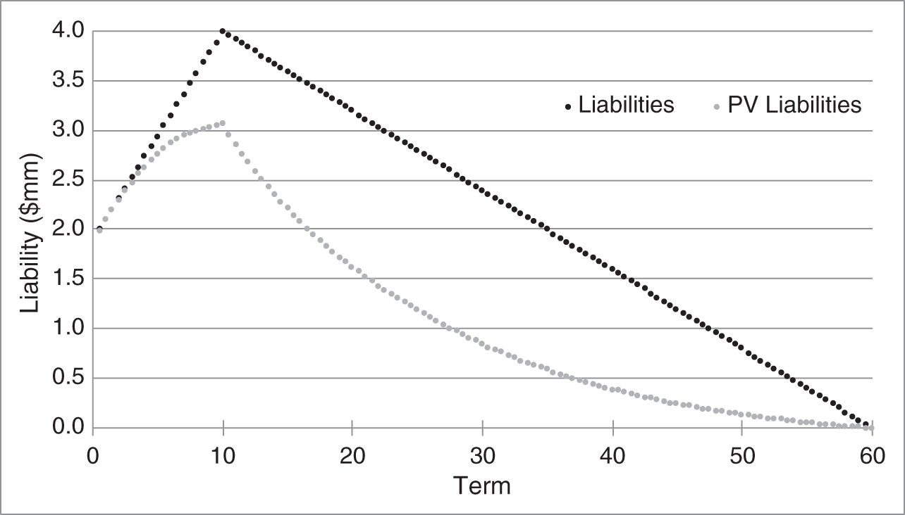
FIGURE 4.10 Liabilities of a Stylized Defined‐Benefit Pension Fund. Present Values Are Computed by Discounting at the HQM Curve, as of May 2021.
Because many pension funds make future payment commitments in line with returns on corporate bonds, the considerations in the previous paragraph lead many funds to invest a significant portion of their funds in corporate bonds. For the purposes of this section, it is assumed that all of the $140 million of pension assets are invested in corporate bonds. More specifically, it is assumed that the pension fund can invest in one or two of the Johnson & Johnson (JNJ) bonds listed in Table 4.6. As mentioned in Chapter 3, all of these bonds were issued by JNJ in August 2020. For expository purposes, these bonds are referred to by their original terms, which are not that different from their terms as of mid‐May 2021. For example, the 0.55s of 09/1/2025 are called the five‐year bonds, while the 2.45s of 09/1/2060 are called the 40‐year bonds. The durations and convexities in the table are all yield‐based metrics.
The duration and convexity of the pension liabilities, computed by a parallel shift in the HQM par rate curve, are 16.66 and 211.37, respectively. To hedge against the risk that rates fall, which would increase the present value of the liabilities, the pension fund decides to invest in an asset portfolio with a duration of 16.66, the duration of the liabilities. But in which of the JNJ bonds should the fund invest?
Perhaps the most straightforward answer is to invest in the 20‐year bonds, which have a duration of 15.56. With its assets invested in this bond, the fund would have an asset duration equal to that of the bond, 15.56, and a liability duration, given already, of 16.66. Were rates to fall by 100 basis points, then, along the lines of previous sections, assets would increase in value by approximately 15.56% and liabilities by approximately 16.66%. The result is close to hedged, but not quite. On the initial portfolio value of $140 million, the present value of the liabilities would then exceed the value of the assets by ![]() × $140 million, or 1.1% of value, or $1,540,000.
× $140 million, or 1.1% of value, or $1,540,000.
TABLE 4.6 Selected Johnson & Johnson Bond Issues. Yields, Durations, and Convexities Are as of Mid‐May 2021. Coupons and Yields Are in Percent.
| Coupon | Maturity | Yield | Duration | Convexity |
|---|---|---|---|---|
| 0.55 | 09/1/2025 | 0.717 | 4.23 | 10.06 |
| 0.95 | 09/1/2027 | 1.238 | 6.08 | 20.33 |
| 1.30 | 09/1/2030 | 1.846 | 8.69 | 41.31 |
| 2.10 | 09/1/2040 | 2.686 | 15.56 | 141.49 |
| 2.25 | 09/1/2050 | 2.849 | 20.72 | 269.41 |
| 2.45 | 09/1/2060 | 2.962 | 24.09 | 393.17 |
To clean up that hedge, the pension fund might use cash. Denote the amount held in cash by ![]() , so that the fund's remaining funds,
, so that the fund's remaining funds, ![]() , are invested in the 20‐year bond. Then, as mentioned in Section 4.4, the duration of this portfolio is the weighted average of its component durations. Note, too, that the duration of cash equals zero: its present value always equals its amount, no matter how rates change. Therefore, setting the duration of this asset portfolio equal to the duration of the liabilities,
, are invested in the 20‐year bond. Then, as mentioned in Section 4.4, the duration of this portfolio is the weighted average of its component durations. Note, too, that the duration of cash equals zero: its present value always equals its amount, no matter how rates change. Therefore, setting the duration of this asset portfolio equal to the duration of the liabilities,
Solving, ![]() , meaning that the pension fund would borrow $9.90 million, or about 7% of the $140 million, and invest
, meaning that the pension fund would borrow $9.90 million, or about 7% of the $140 million, and invest ![]() or about 107% in the 20‐year bond.
or about 107% in the 20‐year bond.
The asset portfolio just described hedges the duration risk of the liabilities. But how does the convexity of the asset portfolio compare with the convexity of the liabilities? As mentioned in Section 4.5, the convexity of a portfolio is the weighted average of the convexity of its components. Here, with the convexity of cash equal to zero and the convexity of the 20‐year bond equal to 141.49, the convexity of the asset portfolio is,
which is less than the convexity of the liabilities, given earlier as 211.37. Hence, this asset portfolio results in the pension fund having an overall negatively convex position. Figure 4.11 graphs the P&L of this asset portfolio and of the liabilities, where the P&L of the bond is calculated as a shift in its yield, and the P&L of the liabilities by parallel shifts in the HQM par rate curve. As rates fall, the values of both the liabilities and the asset portfolio increase, as envisioned by the duration hedge. Because of the duration hedge, in fact, the values of both increase by about the same amount for relatively small rate changes. But because the liabilities have a higher convexity, the duration of the liabilities increases more as rates decline. Therefore, for large declines in rates, the increase in value of the liabilities is greater than the increase in value of the assets, which leaves the pension fund with a net loss in value.
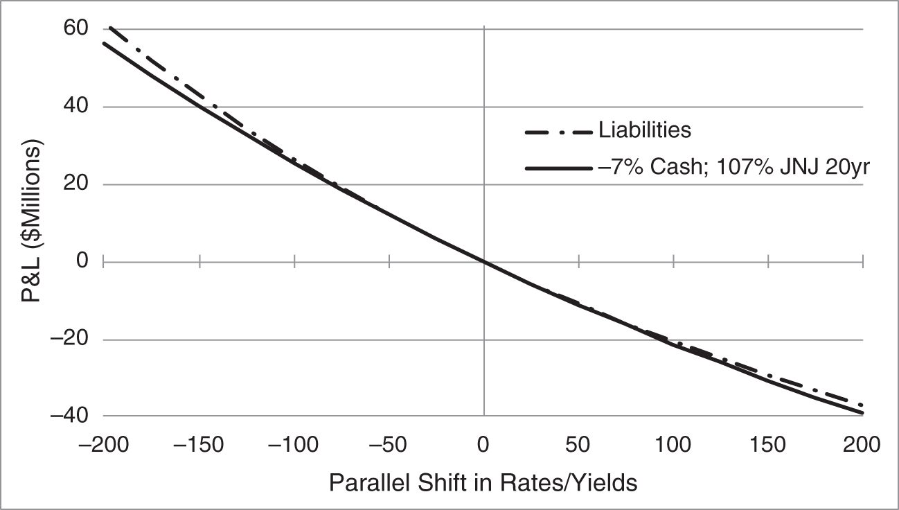
FIGURE 4.11 P&L of the Pension Fund Liabilities in Figure 4.10 and of a Portfolio Borrowing $9.90 Million and Investing $149.90 Million in the Johnson & Johnson 2.10s of 09/1/2040. The P&L of the Liabilities Is Computed Under a Parallel Shift of HQM Par Rates. The P&L of the Bond Is Computed by a Shift in Its Yield.
As rates increase, the values of both the liabilities and the asset portfolio fall, again as envisioned by the duration hedge. But because the liabilities have a higher convexity, the duration of the liabilities falls more as rates increase. Therefore, for large increases in rates, the fall in the value of the liabilities is less than the fall in value of the assets, which, again, leaves the pension fund with a net loss in value.
The pension fund could manage this negative convexity by adjusting its hedge as rates change. As rates fall, and the duration of the liabilities increases more than the duration of the assets, the fund could increase its asset duration by borrowing more cash and buying more bonds. As rates rise, and the duration of the liabilities falls more than that of the assets, the fund could lower its asset duration by selling bonds and paying off some of its borrowing. This solution is fine in theory and sometimes in practice, but it is costly in the sense of requiring potentially frequent portfolio rebalancing.
Another approach is to find an asset portfolio that not only matches the duration of the liabilities, but that also has a convexity equal to or greater than that of the liabilities. There are, of course, many such portfolios that can be formed from cash and the JNJ bonds listed in Table 4.6. For discussion purposes, Table 4.7 lists the portfolio already discussed, along with two additional, two‐asset portfolios.
TABLE 4.7 Selected Portfolios of JNJ Bonds Listed in Table 4.6 That Match the Duration of the Liabilities in Figure 4.10, as of Mid‐May 2021. Bond Duration and Convexity Are Calculated with Parallel Shifts in Yields. Proportions and Yields Are in Percent.
| Wtd‐Avg | ||||||
|---|---|---|---|---|---|---|
| Asset | Proportion | Asset | Proportion | Yield | Duration | Convexity |
| Cash | −7.05 | 2.10s of 2040 | 107.05 | 2.87 | 16.66 | 151.47 |
| 0.55s of 2025 | 24.66 | 2.25s of 2050 | 75.34 | 2.32 | 16.66 | 205.47 |
| Cash | 30.86 | 2.45s of 2060 | 69.14 | 2.06 | 16.66 | 271.84 |
Each row gives the two assets in the portfolio; the proportion of value in each asset; the weighted‐average yield of the portfolio, with weights equal to the proportions of value; the duration of the portfolio; and the convexity of the portfolio. The weighted‐average yield of the portfolio is far from a perfect measure of ex‐ante portfolio return, but will serve for the purposes of this section. Cash, consistent with market levels at the time, is assumed to have a yield of 0.05%. Portfolio duration and convexity equals the weighted average of the duration and convexity of the components, as explained earlier in the chapter.
The first row of the table corresponds to the asset portfolio already analyzed. Its duration equals 16.66, which equals the duration of the liabilities, but its convexity is significantly less than 211, the convexity of the liabilities. The second row gives a portfolio invested in the five‐year and 30‐year bonds, with the proportions such that the duration of the asset portfolio matches that of the liabilities. The convexity of the portfolio is 205.47, which is quite close to the 211.37 convexity of the liabilities. The third row gives an asset portfolio that once again matches the duration of the portfolio, this time by investing much more in cash and the residual in the 40‐year bond. This portfolio has a convexity of 271.84, which exceeds that of the liabilities.
The relative convexities of the asset portfolios in Table 4.7 illustrate the following general principle: among portfolios with the same duration, the more spread out the cash flows of a portfolio, the greater its convexity. All portfolios in the table are constructed to have the same duration, but the first portfolio is essentially all in the 20‐year bond. In the asset–liability management context, this portfolio is called a bullet portfolio: the liability cash flows, which are spread over many years, are being hedged by a single bond with matching duration. The second asset portfolio in the table is split between five‐year and 30‐year bonds, while the third is split between cash – essentially a zero‐year bond – and 40‐year bonds. These two portfolio are called barbell portfolios, because they are hedging liabilities using one bond with less duration than the liabilities and one bond with more.
Matched‐duration portfolios with cash flows that are more spread out have greater convexities because, as explained earlier, duration is roughly linear in term, while convexity is quadratic. Consider a 10‐year zero coupon bond at a yield of zero, which, according to Equations (4.28) and (4.33), has a duration of 10 and a convexity of ![]() . By contrast, a portfolio with 50% of its value in a five‐year zero coupon bond and 50% in a 15‐year zero, using the same equations, also has a duration 10, but a convexity of 50% times the convexity of the five‐year zero, 22.5, plus 50% times the convexity of the 15‐year zero, 232.5, which equals 127.5. Because convexity is quadratic in term, the convexity of the 15‐year zero dominates. Hence, the portfolio with the more spread‐out cash flows – the one with the longest‐term bond – has the greatest convexity.
. By contrast, a portfolio with 50% of its value in a five‐year zero coupon bond and 50% in a 15‐year zero, using the same equations, also has a duration 10, but a convexity of 50% times the convexity of the five‐year zero, 22.5, plus 50% times the convexity of the 15‐year zero, 232.5, which equals 127.5. Because convexity is quadratic in term, the convexity of the 15‐year zero dominates. Hence, the portfolio with the more spread‐out cash flows – the one with the longest‐term bond – has the greatest convexity.
Given the calculations in Table 4.7, how should the pension fund choose among the alternatives? Figure 4.12 graphs the net P&L of the liabilities and each of the asset portfolios. The net P&L of the liabilities and the bullet portfolio, ![]() 7% in cash and 107% in the 20‐year bond, is clearly negatively convex: it loses value whether rates fall or rise. The barbell portfolio with 25% in the five‐year bond and 75% in the 30‐year bond, which matches the duration and approximately matches the duration of the liabilities, gives rise to a net P&L that is very small over a wide range of rates. In other words, a pension fund with this portfolio need not rebalance its asset portfolio unless rates fall significantly. Lastly, the barbell portfolio with 31% in cash and 69% in the 40‐year, gives rise to an overall, positively convex position. The combination of assets and liabilities gains value whether rates fall or rise.
7% in cash and 107% in the 20‐year bond, is clearly negatively convex: it loses value whether rates fall or rise. The barbell portfolio with 25% in the five‐year bond and 75% in the 30‐year bond, which matches the duration and approximately matches the duration of the liabilities, gives rise to a net P&L that is very small over a wide range of rates. In other words, a pension fund with this portfolio need not rebalance its asset portfolio unless rates fall significantly. Lastly, the barbell portfolio with 31% in cash and 69% in the 40‐year, gives rise to an overall, positively convex position. The combination of assets and liabilities gains value whether rates fall or rise.
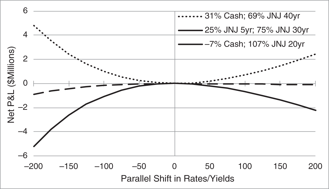
FIGURE 4.12 Net P&L of the Pension Fund Liabilities in Figure 4.10 and the Asset Portfolios in Table 4.7. The P&L of the Liabilities Is Computed Under a Parallel Shift of HQM Par Rates. The P&L of the Bond Is Computed by a Shift in Its Yield.
Does Figure 4.12 prove that the pension fund should always choose the most convex asset portfolio? The answer is no. As mentioned in Section 4.6, evaluating P&L purely as a function of changes in rates does not account for the passage of time. As a rough proxy for return as time passes with rates unchanged, consider the weighted‐average yields in Table 4.7, which fall with convexity. In other words, markets recognize the contribution of convexity to P&L as rates change, as shown in Figure 4.12, and, therefore, offer lower yields for highly convex portfolios. As a result, a portfolio with relatively low convexity and relatively high yield underperforms if rates change a lot but outperforms if rates stay about the same. By contrast, a portfolio with relatively high convexity and relatively low yield outperforms if rates change a lot but underperforms if rates stay about the same.
Figure 4.13 illustrates the trade‐off between yield and convexity by graphing the yields of the JNJ bonds from Table 4.6 against their durations. The curve has a concave shape, meaning that any line connecting two points on the curve is below the curve. Now, in the context of this graph, compare the second portfolio from Table 4.7 – the barbell of the five‐year and 30‐year bonds – versus the bullet 20‐year bond portfolio. The barbell portfolio, with a duration of 16.66 and a weighted‐average yield of 2.32%, corresponds to the point on the dotted line at a duration of 16.66. By the concavity of the yield‐duration curve, this yield is very much below the yield of the 20‐year bond, which has a similar duration.4 More generally, the concavity of the duration‐yield curve implies that the weighted‐average yield on portfolios with more spread‐out component bonds, which are more convex portfolios, is lower than the yield of bullet portfolios and also of less spread‐out – less convex – portfolios. Chapter 8 demonstrates more formally how the shape of the term structure ensures that the benefits of convexity are fairly offset by lower return.
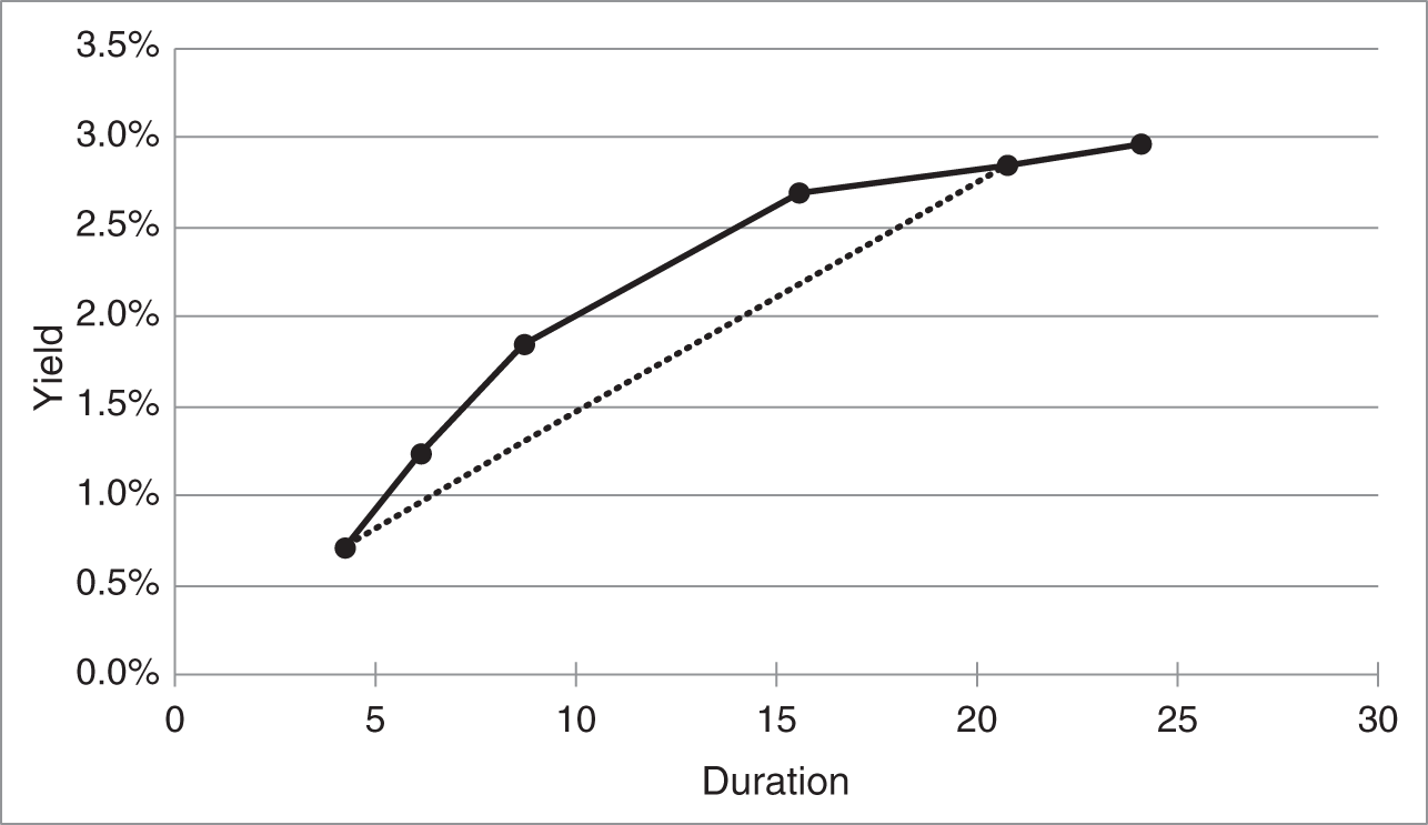
FIGURE 4.13 Yields of the Johnson & Johnson Bonds in Table 4.6 Against Their Durations.
Given the discussion in the last several paragraphs, a pension fund manager who decides to match the duration of assets and liabilities has to decide whether to trade yield for positive convexity. An asset portfolio with a relatively low yield but convexity exceeding that of the liabilities does not have to be rebalanced often to avoid losses, does relatively well when rates move a lot, and does relatively poorly when rates do not move much. An asset portfolio with a relatively high yield but convexity less than that of the liabilities has to be rebalanced often to avoid losses, does relatively poorly when rates move a lot, and does relatively well when rates do not move much. To summarize, then, the choice actually depends on whether rates will change by much or not, that is, on future interest rate volatility!
NOTES
- 1 This terminology is a historical artifact. The first metric of this sort was Macaulay duration, which equals the expressions in (4.24) or (4.25) ×
 . Over time, however, the definitions in the text became the industry standard. Macaulay duration has the advantage that the resulting duration of a zero coupon bond is exactly equal to its years to maturity. The definitions in the text, however, have the advantage that they are exactly equal to the percentage change in price for a change in rates.
 - 2 A purely mathematical reason that the units of duration is years is that duration is a percentage change divided by a change in interest rate per year.
- 3 While usually the case, it is not true that duration of any bond always increases with term. The durations of deeply discounted coupon bonds increase with term, arbitrarily close to the zero coupon line in Figure 4.7, but can then decline, with further increases in term, as the duration falls to that of a perpetuity. The duration of a perpetuity is the reciprocal of the yield, which can be shown letting
 approach infinity in Equations (4.21) and (4.25).
 - 4 This is a bit imprecise: the duration of the 20‐year bond is actually 15.56, while the bullet portfolio has a duration of 16.66.