
CHAPTER 5
Key‐Rate, Partial, and Forward‐Bucket '01s and Durations
The assumption in Chapter 4 that changes in the entire term structure can be described by one interest rate factor may be convenient and appropriate in certain situations, but applications with exposures across the term structure require more realistic foundations. Consider a life insurance company that has liabilities spread out over many years in the future. The insurer could make assumptions about how rates across the term structure typically vary with the 10‐year par rate and then hedge all of its liabilities by buying 10‐year bonds. But what if, over a particular period, the 30‐year rate falls and the 10‐year rate stays the same? The present value of liabilities would increase, asset value would be unchanged, and the insurer would experience a net loss in value.
Given that a one‐factor framework cannot reliably describe rate changes across the term structure, market participants have pursued three broad strategies. First, build a multi‐factor term structure model, based on a combination of data and market analysis. Many active hedge funds and asset managers, who build such models for investment purposes anyway, pursue this path for hedging as well. The Gauss+ model presented in Chapter 9 is an example of this approach. Second, hedge based on empirical analyses of relationships across rates of various terms. Examples of this approach are given in Chapter 6. Third, adopt a robust approach to hedging, which performs well regardless of how the term structure evolves but which leaves little room for subjective views and gives no guidance as to investment decisions. Many asset–liability managers and market makers, who do not see themselves in the business of taking views on term structure movements, pursue this path, which is the subject of this chapter.
The extreme of robust approaches to hedging is immunization, that is, hedging away the risk of every single cash flow. An example would be buying eight zero coupon bonds to fund eight semesters of college tuition payments. No matter what happens to interest rates and the term structure, the maturing zero coupon bonds will fund the assumed payments. Immunization is not practical, however, in many institutional contexts. An insurance company has too many liabilities on too many future dates for each of them to be funded – and therefore hedged – individually. Aside from the operational costs of such a program, the transaction costs of buying relatively small quantities of so many different fixed income securities is likely to be prohibitive.
Practical approaches to robust hedging, therefore, incorporate enough factors to ensure acceptable performance under a wide range of term structure scenarios but limit the number of factors to maintain tractability and contain transaction costs. The three approaches described in this chapter – key‐rate '01s and durations, partial '01s – and forward‐bucket '01s, have proved popular as striking a sensible balance between hedging effectiveness and practicality or cost. The final section of the chapter briefly connects multi‐factor exposures with portfolio volatility.
5.1 KEY RATES: MOTIVATION
The main motivation for multi‐factor hedging is to control curve risk, that is, the risk that rates across the term structure do not move in parallel or in any fixed relationship. Figure 5.1 illustrates this phenomenon using changes in the term structure of on‐the‐run US Treasury yields on selected days in June 2021. (On‐the‐run bonds are the most recently issued bonds – and usually the most liquid – in their respective maturity ranges.) Each point on each curve represents a change in an on‐the‐run Treasury yield over a business day. The 20‐year term point on the June 18, 2021, curve, for example, shows that the yield of the on‐the‐run 20‐year Treasury bond fell by 9.7 basis points from June 17, 2021, to June 18, 2021.
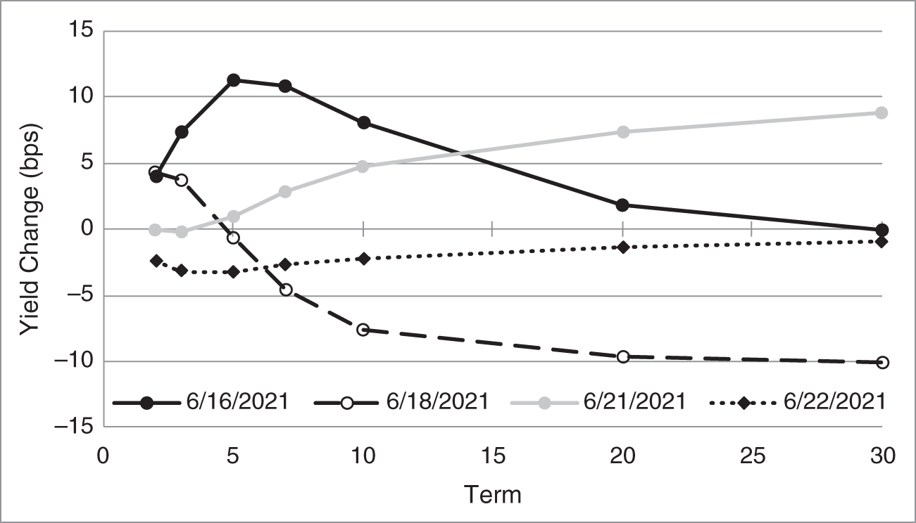
FIGURE 5.1 Changes in the Term Structure of On‐the‐Run US Treasury Yields, Selected Days, June 2021.
The June 16, 2021, curve shows a significant change in the curvature of the term structure: short‐term rates rose some; intermediate‐term rates rose a lot; and long‐term rates rose very little. The June 18, 2021, curve is an example of a flattening of the term structure: short‐term rates rose, intermediate rates fell some, and long‐term rates fell a lot. The June 21, 2021, curve is an example of a steepening: short‐term rates stayed about the same, while longer‐term rates rose significantly. And finally, the June 22, 2021, curve can be very roughly categorized as a parallel shift. From Figure 5.1 as a whole, hedges constructed with the single‐factor metrics of Chapter 4 would not have performed reliably over several days in the second half of June 2021.
5.2 KEY RATES: OVERVIEW
Key‐rate '01s, or key‐rate DV01s, along with key‐rate durations, are designed: i) to describe how the risks of a bond portfolio are distributed along the term structure, and ii) to hedge those risks using some set of bonds, usually the most liquid government bonds of various maturities. To introduce the topic, Table 5.1 shows the key‐rate durations for the JPMorgan Government Bond Fund and its benchmark portfolio, the Bloomberg‐Barclays US Government Bond Index, as of May 31, 2021. The “Total” durations, in the last row of the table, have similar interpretations as the yield‐based durations of Chapter 4. The JPM fund's total duration of 5.73 means that its value increases by approximately 5.73% for a parallel decline in par rates of 100 basis points. The JPM fund, therefore, has less duration risk than its benchmark, which has a duration of 6.78. The other rows of the table give the key‐rate durations of these two bond portfolios. From the “5yr” row, for example, the JPM fund increases in value by approximately 0.80% when the five‐year par rate declines by 100 basis points, but all other par rates remain unchanged. Similarly, from the 20‐year row, the benchmark portfolio increases in value by approximately 1.67% when the 20‐year par rate declines by 100 basis points, but all other par rates remain unchanged.
TABLE 5.1 Key‐Rate Durations of JPMorgan Government Bond Fund and Its Benchmark Portfolio, the Bloomberg‐Barclays US Government Bond Index, as of May 31, 2021.
| JPM Government | Bloomberg‐Barclays | |
|---|---|---|
| Key Rate | Bond Fund | Government Bond Index |
| 6mo | 0.03 | – |
| 1yr | 0.11 | 0.11 |
| 2yr | 0.19 | 0.34 |
| 3yr | 0.40 | 0.60 |
| 5yr | 0.80 | 0.88 |
| 7yr | 1.19 | 0.86 |
| 10yr | 1.31 | 0.57 |
| 20yr | 1.05 | 1.67 |
| 30yr | 0.65 | 1.75 |
| Total | 5.73 | 6.78 |
The key‐rate duration profile of a portfolio, therefore, decomposes its total duration, that is, its sensitivity to parallel shifts in par rates, into separate durations or sensitivities to changes in individual par rates. Consistent with key‐rate durations as a decomposition of total duration, the sum of all key‐rate durations of a portfolio is equal or very nearly equal to the total duration of the portfolio.
The key‐rate duration profiles in the table say a lot about the exposures of the two portfolios to par rates of different terms. The interest rate risk of the JPM fund is somewhat concentrated in seven‐ to 20‐year par rates, while the risk of the index is concentrated in five‐ to seven‐year and, even more so, in 20‐ to 30‐year rates. Part of the reason for the relative differences in these exposures is that the JPM fund invests in US agency mortgage‐backed securities, which are particularly sensitive to seven‐ to 10‐year rates, while the benchmark index contains only government bonds. In any case, as a result of these key‐rate duration differences, the two portfolios will perform differently as the shape of the term structure fluctuates.
The JPM fund reports exposures to the nine key rates listed in Table 5.1. The index fund reports only eight key rates, leaving out the six‐month rate. The number of key rates chosen involves a trade‐off, along the lines of the introduction. With too few key rates, the term structure is likely to move in a way not captured by the framework. With too many, risk management becomes cumbersome and costly.
Along with the number of key rates, the terms of the key rates need be chosen. Because key‐rate DV01s and durations are designed to be hedged with a relatively small set of liquid bonds, the most popular choices for key rates are those that correspond to the maturities of on‐the‐run Treasuries. Including the Treasury's regular issuance of six‐month and one‐year bills, along with its regular issuance of two‐, three‐, five‐, seven‐, 10‐, 20‐, and 30‐year bonds, the JPM and index funds in Table 5.1 have clearly made this popular choice.
5.3 KEY RATES: SHIFTS
The next section applies key‐rate metrics and hedging to the problem of the pension fund introduced in Section 4.8. To keep the exposition simple, and to dovetail with the pension fund's long‐term liabilities and intention to invest in the Johnson & Johnson (JNJ) bonds listed in Table 4.6, the analysis here is restricted to four key rates with terms of 10, 20, 30, and 40 years.
The key‐rate framework imposes no restrictions on how any key rate changes relative to another. But in order to reprice any bond after any shift of key rates, the framework must specify how all par rates move, not just how key rates move. To that end, key‐rate analysis makes the following assumptions: i) each key‐rate shift leaves all other key rates unchanged; ii) each key‐rate shift changes only those par rates that are between adjacent key rates; and iii) changes in par rates due to a key‐rate shift decline linearly from the change in that key rate to zero at adjacent key rates. The resulting shifts, in the current example, are shown in Figure 5.2.
The 20‐year key‐rate shift, depicted by the black, dashed line in the figure, equals one basis point at a term of 20 years. That shift has no effect on par rates with terms less than 10 years – the term of the previous key rate – or on par rates with terms greater than 30 years – the term of the next key rate. Between 10 and 30 years, however, the impact of the shift declines linearly from the 20‐year term, which, since the adjacent key rates are both 10 years distant, means a decline of 0.1 basis points per year. For example, the shift increases the 19‐ and 21‐year par rates by 0.9 basis points each; the 18‐ and 22‐year rates by 0.8 basis points each; etc., the 11‐ and 29‐year rates by 0.1 basis points each; and the 10‐ and 30‐year par rates, which are the adjacent key rates, by 0.0 basis points each.
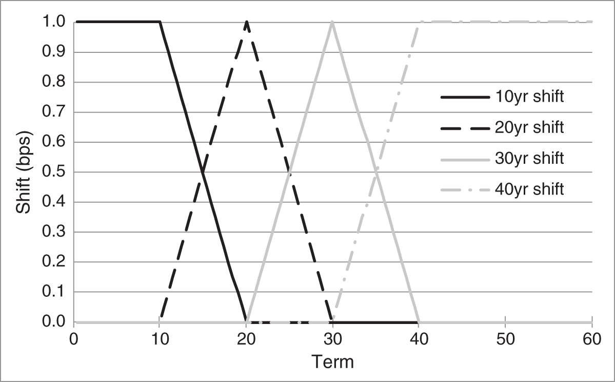
FIGURE 5.2 Key Rate Shifts with Four Key Rates at Terms of 10, 20, 30, and 40 Years.
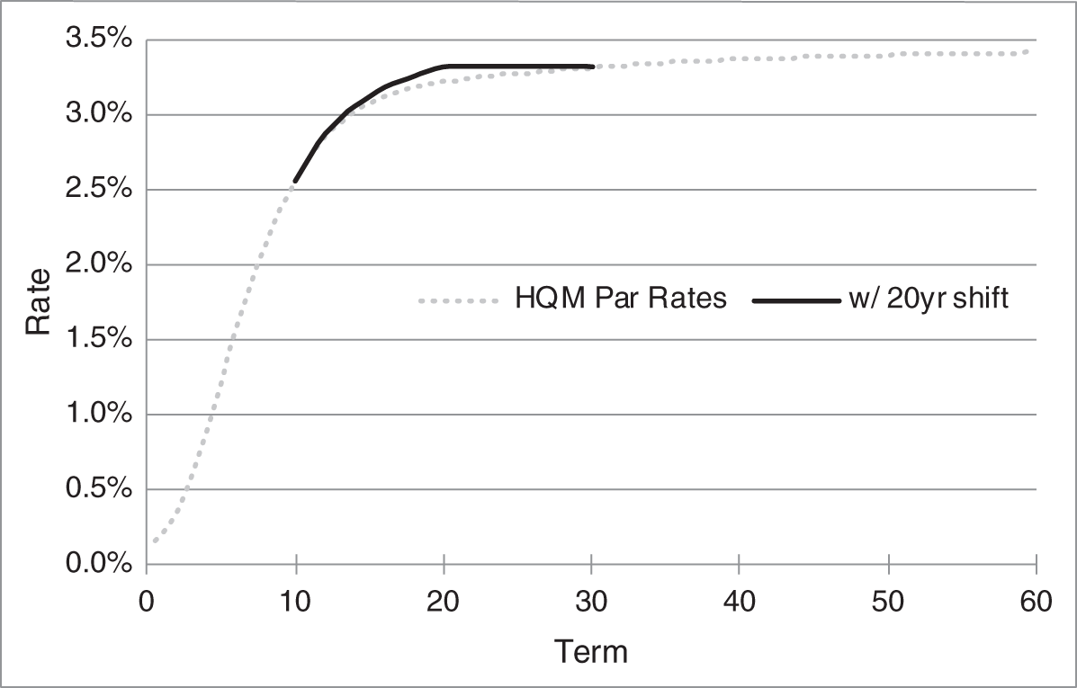
FIGURE 5.3 The HQM Par Rate Curve, as of May 2021, with and Without a 20‐Year Key‐Rate Shift.
When computing the 20‐year key‐rate DV01 or key‐rate duration of a bond or portfolio, all prices are recomputed after shifting the existing par rate curve by the 20‐year key‐rate shift. Figure 5.3 shows the starting High‐Quality Market‐Weighted (HQM) corporate par‐rate curve as the gray, dotted line, and the 20‐year key‐rate shift, just described, added to that par‐rate curve. The shifted par‐rate curve, therefore, is the dotted line out to 10 years, the black line from 10 to 30 years, and the dotted line again from 30 to 60 years. As an aside, while this shifted par‐rate curve looks reasonable enough, spot and forward rates implied by this shifted curve may not look as natural or reasonable.
The 30‐year key‐rate shift in Figure 5.2 is constructed like the 20‐year shift. The shift equals one basis point at 30 years and declines linearly on both sides, at 0.1 basis points a year, because the adjacent key rates – at 20 and 40 years – are each 10 years distant. The 10‐year and 40‐year shifts are constructed somewhat differently, because there is no key‐rate at a term less than 10 years or greater than 40 years. The 10‐year shift, therefore, equals one basis point for all par rates with terms less than 10 years, and the 40‐year shift equals one basis point for all par rates with terms greater than 40 years.
Were all the shifts in Figure 5.2 to occur simultaneously, the result would be a parallel shift of one basis point. This is obvious for par rates of terms less than or equal to 10 years. For terms between 10 and 20 years, which are affected by the 10‐ and 20‐year shifts, note the following. The 10‐year shift, which starts at one basis point at 10 years, decreases by 0.1 basis points per year. At the same time, the 20‐year shift, which starts at zero at 10 years, increases by 0.1 basis points per year. Hence, the decrease and increase cancel, leaving the shift at one basis point. With similar logic, it is easy to see that simultaneous shifts of all the key rates do result in a parallel shift. This observation explains the sense in which key‐rate '01s and key‐rate durations decompose the DV01 and duration of Chapter 4: each key‐rate exposure is that part of the overall exposure arising from a change in that key rate, holding all other key rates constant.
This section concludes by emphasizing that the assumptions invoked to compute the shifts of par rates between key rates are for convenience rather than to capture market or empirical realities. Most obviously, there is no reason to think that par rates respond linearly to changes in adjacent key rates. More subtly, the assumption that par rates are affected only by adjacent par rates is restrictive as well. If, for example, the 10‐year rate falls, while the 20‐ and 30‐year rates stay the same, the 25‐year rate might very well change so that the overall shape of the term structure continues to be reasonable. In any case, despite these objections, the formulation of key‐rate shifts described here has been widely accepted as a sensible trade‐off between reality and tractability.
5.4 KEY RATES: '01S, DURATIONS, AND HEDGING
Unlike their one‐factor equivalents in Chapter 4, key‐rate DV01s and durations are based on change in price, or percentage change in price, for a change in a single key rate. Mathematically, the DV01 and duration with respect to key rate ![]() are defined as,
are defined as,
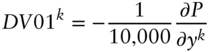
where ![]() denotes the partial derivative of price with respect to that one key rate. For example, the price of the JNJ 2.10s of 09/1/2040 is 91.2209, at which price its spread to the HQM par‐rate curve is
denotes the partial derivative of price with respect to that one key rate. For example, the price of the JNJ 2.10s of 09/1/2040 is 91.2209, at which price its spread to the HQM par‐rate curve is ![]() 0.514%. After a 20‐year key‐rate increase of one basis point, the price of the bond – at the same spread – falls to 91.0790. Therefore, the bond's 20‐year key‐rate '01 is,
0.514%. After a 20‐year key‐rate increase of one basis point, the price of the bond – at the same spread – falls to 91.0790. Therefore, the bond's 20‐year key‐rate '01 is,
and its 20‐year key‐rate duration is,
TABLE 5.2 Key‐Rate DV01s and Hedging of the Pension Liabilities in Figure 4.10 with Par Bonds as of Mid‐May 2021.
| Pension | 2.560s of | 3.215s of | 3.309s of | 3.365s of | |
|---|---|---|---|---|---|
| Liabilities | 05/15 | 05/15 | 05/15 | 05/15 | |
| ($) | 2031 | 2041 | 2051 | 2061 | |
| PV/Price | 139,786,479 | 100 | 100 | 100 | 100 |
| 10yr Shift | 33,192 | 0.09125 | 0 | 0 | 0 |
| 20yr Shift | 52,969 | 0 | 0.15282 | 0 | 0 |
| 30yr Shift | 57,786 | 0 | 0 | 0.19508 | 0 |
| 40yr Shift | 88,766 | 0 | 0 | 0 | 0.22437 |
| Total | 232,713 | 0.09125 | 0.15282 | 0.19508 | 0.22437 |
| Hedge Face | |||||
| Amount ($millions) | 36.375 | 34.661 | 29.622 | 39.562 | |
Table 5.2 takes a preliminary step in using key rates for asset – liability management in the context of the pension fund introduced in Section 4.8. The first column gives the key‐rate DV01s of the pension liabilities in Figure 4.10. The total present value of the pension liabilities is about $140 million, and the DV01 of those liabilities is $232,713. The key‐rate DV01s decompose that total DV01 into exposures to the four key rates. A 10‐year shift of minus one basis point increases the present value of the liabilities by $33,192; a 20‐year shift of minus one basis point increases value by $52,969; and so forth. The exposure to the 10‐year shift is relatively low because, as evident from Figure 4.10, the liabilities build up gradually over the first 10 years and because the values of cash flows of relatively near terms have relatively low interest rate sensitivities. The exposure to the 40‐year key‐rate shift is relatively high because, unlike the other shifts, it affects 30 years of cash flows – from 30 to 60 years out – and because the values of those distant cash flows have relatively high interest rate sensitivities.
For expositional purposes, four fictional bonds are created for the rest of the table. (After these results are discussed, the analysis returns to the JNJ bonds.) The maturities of these fictional bonds are chosen to match the terms of the key rates exactly, that is, 10, 20, 30, and 40 years, and their coupons are chosen so that their prices are all par under the HQM par‐rate curve in May 2021.
Given the careful selection of these bonds, each has exposure only to the key rate corresponding to its maturity. The 2.560s of 05/15/2031, for example, as of May 15, 2021, are exactly 10‐year par bonds. Their price changes only if the 10‐year par rate changes. But, by construction, the 20‐year, 30‐year, and 40‐year shifts do not change the 10‐year par rate. Therefore, the 2.560s have exposure only to the 10‐year shift, and that exposure also equals the bond's total exposure. With the same logic applying to the other three bonds, key‐rate '01s are nonzero only when the term of the key rate equals the maturity of the bond.
Because each of the bonds has such a simple key‐rate '01 profile, computing the key‐rate hedge of the pension liabilities is correspondingly simple. The objective of the hedge is to purchase an asset portfolio that offsets the key‐rate exposures of the liabilities. More specifically, the asset portfolio must have a DV01 exposure to the 10‐year shift of $33,192; to the 20‐year shift of $52,969; etc. But because the only bond that has any exposure to the 10‐year shift is the 2.560s of 05/15/2031, the full exposure to that shift has to come from that bond. Mathematically, denoting the face amount of the 10‐year bond by ![]() ,
,
Solving, ![]() is about $36.375 million, which is listed in the bottom row of Table 5.2. Proceeding analogously to hedge the next three key‐rate exposures, the equations are,
is about $36.375 million, which is listed in the bottom row of Table 5.2. Proceeding analogously to hedge the next three key‐rate exposures, the equations are,
Each of these equations can be solved on its own to find the hedge face amounts recorded in the table.
To summarize, because the hedging bonds are par bonds with maturities equal to the terms of the key rates, key‐rate hedges can essentially be read off the table. The pension fund must purchase $33,192 in DV01 from 10‐year par bonds; $52,969 in DV01 from 20‐year par bonds; and so forth. In this way, the pension fund will be hedged against any combination of key‐rate shifts. The four key rates do not need to move according to any model or predetermined pattern. The 10‐year key rate might move by +8 basis points, the 20‐year by +2 basis points, the 30‐year by 0 basis points, and the 40‐year by ![]() 2 basis points (i.e., something like the May 16, 2021, shift in Figure 5.1), and the hedge should perform relatively well. The caveat, of course, is that the performance can be eroded to the extent that rates between the key rates change in a way markedly different from the shapes of the shifts in Figure 5.2. This caveat, however, is more of an issue in this simplified example, with only four key rates over a maturity range of 60 years, than it is in practice, for example, with the eight or nine key rates over a maturity range of 30 years used by the JPM Government Bond Fund and the Bloomberg‐Barclays US Government Bond Index in Table 5.1.
2 basis points (i.e., something like the May 16, 2021, shift in Figure 5.1), and the hedge should perform relatively well. The caveat, of course, is that the performance can be eroded to the extent that rates between the key rates change in a way markedly different from the shapes of the shifts in Figure 5.2. This caveat, however, is more of an issue in this simplified example, with only four key rates over a maturity range of 60 years, than it is in practice, for example, with the eight or nine key rates over a maturity range of 30 years used by the JPM Government Bond Fund and the Bloomberg‐Barclays US Government Bond Index in Table 5.1.
TABLE 5.3 Key‐Rate DV01s and Hedging of the Pension Liabilities in Figure 4.10 with Johnson & Johnson Bonds. Indicative Prices Are as of Mid‐May 2021.
| Pension | 1.30s of | 2.10s of | 2.25s of | 2.45s of | |
|---|---|---|---|---|---|
| Liabilities | 09/01 | 09/01 | 09/01 | 09/01 | |
| ($) | 2030 | 2040 | 2050 | 2060 | |
| PV / Price | 139,786,479 | 95.357 | 91.221 | 88.154 | 88.157 |
| HQM Sprd (bps) | 0 | −56.4 | −51.4 | −45.4 | −39.2 |
| 10yr Shift | 33,192 | 0.08577 | 0.00597 | −0.00393 | −0.00250 |
| 20yr Shift | 52,969 | 0 | 0.14191 | 0.00707 | −0.00473 |
| 30yr Shift | 57,786 | 0 | 0 | 0.18494 | 0.00871 |
| 40yr Shift | 88,766 | 0 | 0 | 0 | 0.21548 |
| Total | 232,713 | 0.08577 | 0.14788 | 0.18808 | 0.21695 |
| Hedge Face | |||||
| Amount ($millions) | 38.647 | 37.239 | 29.306 | 41.195 | |
With the basics of key‐rate hedging understood, the fictional par bonds created for Table 5.2 are replaced by the approximately 10‐year, 20‐year, 30‐year, and 40‐year JNJ bonds listed in Table 4.6. The updated analysis is presented in Table 5.3. The row “HQM Sprd” gives the spread of each of the JNJ bonds to the HQM par‐rate curve as of mid‐May 2021. These spreads are all negative, because, with its triple‐A rating, JNJ bonds sell at lower rates than HQM par‐rates, which represent double‐ and single‐A credits. In any case, the bond spreads in the table are kept constant as key‐rate shifts are applied. No spread is attached to the pension fund liabilities, because, by assumption, their present value is computed directly from the HQM par‐rate curve.
A major difference between Table 5.2, which features fictional, par bonds, and Table 5.3, which features the JNJ bonds, is that the key‐rate DV01 profile of the JNJ bonds is more complex. As of mid‐May 2021, the 1.30s of 09/1/2030 mature in less than 10 years, which means that only the 10‐year key‐rate shift affects their valuation. Their key‐rate profile, therefore, is completely concentrated in the risk of a 10‐year shift. The other bonds, however, which do not mature in exactly 20‐, 30‐, and 40‐years and which are not priced at par, have small positive or negative exposures to key rates other than those corresponding most closely to their maturities.
Because the bulk of each bond's exposure is still at the key rate closest to its maturity, the hedging problem in Table 5.3 is not conceptually different from the earlier table. Solving for the hedging portfolio is more tedious, however, because no key‐rate exposure of the liability can be handled in isolation. All of the bonds have exposures to the 10‐year shift; three have exposures to the 20‐year shift; and so forth. Consequently, the following equations (with key‐rate '01s rounded for readability) need to be solved together,
Equation (5.9) says that the combined 10‐year key‐rate '01 of the asset portfolio must offset the 10‐year key‐rate '01 of the liabilities. Equation (5.10) says the same for the 20‐year key rate; Equation (5.11) for the 30‐year key rate; and Equation (5.12) for the 40‐year key rate. The solution, given in the bottom row of Table 5.3, is not the same as that in Table 5.3 but is certainly of the same order of magnitude.
5.5 PARTIAL '01S AND PV01
Interest rate swap trading desks are firmly in the category of market participants that require robust, multi‐factor frameworks for hedging. These desks are mostly market makers in swaps, regularly paying fixed to and receiving fixed from customers, while trying to hedge any residual interest rate and curve risk. In order to value these trading books, swap rate curves are constructed to fit or pass through rates of all terms that trade with significant liquidity. There are typically quite a few of these fitting rates or fitting points, perhaps between 15 to 25, depending on the application and currency. In any case, swap desks often leverage their curve‐building machinery to compute PV01s (i.e., present value of an '01) and partial '01s or partial PV01s. The term PV01 is standard in swap markets, but it is really a synonym for the general conception of DV01 described in the early sections of Chapter 4. The term is likely preferred so as to differentiate between that general conception and yield‐based DV01, which is particularly widespread in bond markets.1
The PV01 of a portfolio of swaps is found as follows: compute its present value with the current swap rate curve; shift all fitted rates by one basis point; refit the curve; recompute the present value; and subtract one present value from the other. The sign convention for PV01 is the same as for DV01: positive numbers mean that value increases when rates fall.
A partial '01 of a portfolio is defined for each rate used to fit the swap curve. To find a partial '01 with respect to a particular fitted rate, compute the present value of the portfolio with the current swap curve; shift that fitted rate, keeping all other fitted rates the same; refit the curve; recompute the present value; and subtract one present value from the other, again observing the usual sign convention.
The advantages and caveats of using key‐rate '01s apply to partial PV01s as well. Partial '01s decompose the overall PV01 into exposures to the individual fitted swap rates. Hedging is simple by construction: given a portfolio's partial '01 with respect to a particular fitted rate, offset that exposure by receiving or paying fixed in a swap whose term corresponds to that fitted rate. In this respect, hedging is actually simpler with partial '01s than with key‐rate '01s. Because new, hedging swaps are always at par (see Chapter 2), each partial '01 can be hedged individually, as in the simplified example of Table 5.2, where key‐rate exposures are hedged with par bonds.
With respect to caveats, refitting a curve after shifting one fitted swap rate, keeping all other fitted rates the same, can result in oddly shaped term structures of swap rates and even more so, of spot and forward rates. Furthermore, additional problems can arise if the curve‐fitting methodology is not local enough, that is, for example, if shifting the 10‐year swap rate, keeping other rates the same, unintentionally moves rates between the fitted five‐ and seven‐year rates. In that case, the present value of a six‐year swap would show an unintended sensitivity to the 10‐year swap rate, and, even though five‐ and seven‐year swap rates are included as hedging instruments, the methodology would call for hedging six‐year swaps not only with five‐ and seven‐year swaps, but also with some amount of 10‐year swaps. This outcome is fine if intended, but not fine if just an artifact of the curve‐fitting methodology. Because the success of using partial '01s is very dependent on the properties of the curve fitting methodology, many market participants are careful to use robust curve fitting methodologies or use forward‐bucket '01s, which are described in the next section.2
Before concluding this section, it is noted that the term CV01 denotes the change in value of a swap for a one‐basis‐point decrease in its coupon or fixed swap rate. CV01 is particularly easy to compute, because a moment's reflection reveals that it is proportional to the sum of the discount factors used to discount the fixed payments of the swap. CV01 and PV01 are quite different conceptually, with the former shifting the coupon and the latter shifting discount rates. The two are sometimes used interchangeably and confused, however, perhaps because they are essentially equal for par swaps, which constitute the bulk of swaps trading activity.3
5.6 FORWARD‐BUCKET '01S
Key‐rate and partial '01s are particularly convenient in that they translate directly into hedging with liquid instruments, whether on‐the‐run or near on‐the‐run Treasuries or swaps of the most liquid terms. But the shifts themselves are not very intuitive. Shifting the 10‐year par rate by a basis point does not mean that the 10‐year segment of the term structure shifts, while all other segments stay constant: shifting the 10‐year par rate has implications for discounting all cash flows out to 10 years. Furthermore, as mentioned earlier, shifting one par rate, while holding all other rates constant, can imply odd shifts in spot or forward rates. Forward‐bucket '01s, by contrast, are more easily interpretable in terms of changes in the shape of the term structure. They do not, however, provide the same direct visibility into hedging with liquid instruments as do key‐rate and partial '01s.
This section illustrates the use of forward‐bucket '01s with reference to the general obligation bonds of the Town of Wellesley, Massachusetts, issued in May 2020.4 Table 5.4 lists the first nine bond series sold at that time. Note that, for the tax reasons explained in Section O.2, it is common for municipalities to issue bonds with a coupon of 5% even though market yields are much lower.
Using the yields in Table 5.4, the analytical tools of Part One can be used to calculate a term structure of forward rates, which is graphed in Figure 5.4.5 The idea behind forward‐bucket '01s is to shift “buckets,” that is, individual segments of the forward term structure, directly. For purposes of exposition, this section breaks the term structure into three segments: one to two years; three to five years; and six to nine years. Figure 5.4 shows, for example, a +10‐basis‐point shift of the three‐ to five‐year segment. In practice, practitioners choose buckets most suitable to their businesses. A money‐market desk, for example, which trades very heavily in short‐term instruments, might have many buckets in the short end of the curve and few further on. A swaps desk, on the other hand, which trades evenly across maturities from one to 30 years, might not have nearly as many buckets in the short end but many more evenly spaced buckets across the rest of the curve.
TABLE 5.4 Selected General Obligation Refunding Bonds Issued by the Town of Wellesley, Massachusetts, in May 2020. Coupons and Yields Are in Percent.
| Maturity | Principal | Coupon | Yield |
|---|---|---|---|
| 06/01/2021 | 1,175,000 | 5.00 | 0.75 |
| 06/01/2022 | 1,205,000 | 5.00 | 0.80 |
| 06/01/2023 | 1,210,000 | 5.00 | 0.84 |
| 06/01/2024 | 1,225,000 | 5.00 | 0.90 |
| 06/01/2025 | 1,235,000 | 5.00 | 0.96 |
| 06/01/2026 | 1,250,000 | 5.00 | 1.01 |
| 06/01/2027 | 1,255,000 | 5.00 | 1.06 |
| 06/01/2028 | 1,265,000 | 5.00 | 1.11 |
| 06/01/2029 | 1,270,000 | 5.00 | 1.18 |
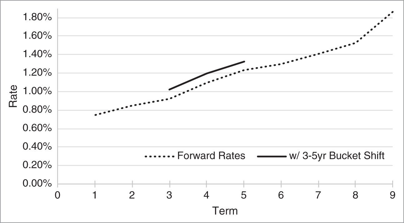
FIGURE 5.4 Town of Wellesley General Obligation Forward Rate Curve with a 10‐Basis‐Point Shift of the Three‐ to Five‐Year Forward Bucket, as of June 1, 2020.
Forward‐bucket '01s are computed analogously to any other interest rate risk metric: price the bond or portfolio with the current term structure; shift a forward‐bucket by one basis point; reprice the bond or portfolio with the new term structure; and subtract one price from another, observing the usual sign convention. Table 5.5 reports forward‐bucket '01 profiles computed along these lines. The second to fourth columns give the forward‐bucket '01s for three of the Wellesley bonds, a two‐year bond, a five‐year bond, and a nine‐year bond, all as of June 1, 2020. For expositional purposes, the fifth column gives the forward‐bucket '01s of a fictional nine‐year par bond, discounted with the same curve. The final row of the table sums all the forward‐bucket '01s, which gives the increase in price after shifting all forward rates down by one basis point. Hence, the forward‐bucket '01s in the table decompose these totals into exposures to individual segments of the term structure.
TABLE 5.5 Forward‐Bucket Exposures and Hedging of Selected Town of Wellesley General Obligation Refunding Bonds, as of June 1, 2020. The 5s of 06/01/2029 are Hedged with the 1.205s of 06/01/2029.
| (1) | (2) | (3) | (4) | (5) | (6) |
|---|---|---|---|---|---|
| Hedged | |||||
| 5s of | 5s of | 5s of | 1.205s of | 5s of | |
| 06/01 | 06/01 | 06/01 | 06/01 | 06/01 | |
| 2022 | 2025 | 2029 | 2029 | 2029 | |
| 1‐2yr Shift | 0.02099 | 0.02324 | 0.02578 | 0.01972 | 0.00239 |
| 3‐5yr Shift | 0 | 0.03112 | 0.03492 | 0.02862 | 0.00098 |
| 6‐9yr Shift | 0 | 0 | 0.03983 | 0.03642 | −0.00337 |
| Total | 0.02099 | 0.05437 | 0.10053 | 0.08475 | 0 |
The two‐year bond, which has no cash flows past two years, has no exposure to the three‐ to five‐year and the six‐ to nine‐year forward‐bucket shifts. Similarly, the five‐year bond has no exposure to the six‐ to nine‐year shift. As intended, forward‐bucket '01s clearly convey exposures to individual segments of the term structure. For example, if forward rates in the three‐ to five‐year segment of the curve fall by one basis point, the price of the 5s of 06/1/2029 increases by 3.5 cents per 100 face amount.
The usefulness of forward‐bucket '01s to assess curve risk is illustrated in the sixth column of Table 5.5. Say that a market maker hedged the 5s of 06/01/2029 with the hypothetically liquid, fictional 1.205s of 06/01/2029 using the parallel shift, that is, the total '01s in the last row of the table. Against a purchase of 100 face amount of the 5s of 06/01/2029, the market maker would sell ![]() of the 1.205s. By definition, the total '01 of this hedged portfolio is zero, but it does have curve risk, which is computed in the last column of the table.
of the 1.205s. By definition, the total '01 of this hedged portfolio is zero, but it does have curve risk, which is computed in the last column of the table.
The exposure of the hedged portfolio to each forward bucket is the sum of the exposures of the two bond positions. For the one‐ to two‐year forward bucket, for example, the portfolio exposure is,
The other two bucket exposures are computed similarly. Taken as a whole, the forward‐bucket '01 profile of the hedged portfolio, with the first two exposures positive and the third negative, shows that the market maker's position loses money if the forward curve flattens. For example, in a particular flattening scenario, if one‐ to five‐year forward rates increase, while six‐ to nine‐year forward rates decrease, the position will lose money due to each of the three forward rate shifts. With curve risk quantified in this way, the market maker can choose between hedging out all curve risk, at some cost, or bearing the risk until the position can be unwound.
Hedging a bond or portfolio with forward‐bucket '01s follows along the same lines as hedging with key‐rate '01s. If there are five forward buckets, for example, then five hedging instruments are required. The five unknowns are the face amount of the five hedging instruments, and each of five equations sets the net '01 of its corresponding forward bucket to zero. While this procedure is perfectly straightforward, an approximate solution is not as immediately apparent as in the case of key‐rate '01s. Inspection of the sixth column of Table 5.5 does not reveal the approximate position of a bond or portfolio of bonds that hedges out the residual curve risk. By contrast, inspection of the dollar key‐rate DV01s in the second column of Table 5.3 readily reveals the approximate trades required in the hedging bonds.
5.7 MULTI‐FACTOR EXPOSURES AND PORTFOLIO VOLATILITY
As discussed in this chapter and Chapter 4, risk metrics are useful for quantifying the effect of a change in rates on prices and for hedging interest rate risk. This section makes the point that risk metrics are also useful for quantifying portfolio volatility.
Say that a portfolio has a DV01 of $10,000 and that interest rates have a volatility of 100 basis points per year. It follows that the portfolio has an annual volatility of $10,000 times 100, or $1 million. This, of course, is a one‐factor formulation of interest rate volatility.
The motivation for multi‐factor exposures, however, is that portfolios are exposed to changes in interest rates all along the curve and that these changes are not perfectly correlated. The discussion here quantifies portfolio volatility in the simple, multi‐factor setting of two key rates. The ideas, however, are easily extended to additional key rates and to partial and forward‐bucket '01s.
To estimate portfolio volatility with two key rates, follow these steps. First, empirically estimate the volatility of changes in each key rate and the correlation between them. Second, compute the key‐rate '01s of the portfolio. Third, compute the variance or volatility of the portfolio. To illustrate this third step, denote the change in the value of the portfolio by ![]() ; the change in the two key rates by
; the change in the two key rates by ![]() and
and ![]() ; and the key rates of the portfolio by
; and the key rates of the portfolio by ![]() and
and ![]() . Then, by the definition of key‐rate '01s,
. Then, by the definition of key‐rate '01s,
Furthermore, denoting the volatility of changes in portfolio value and changes in the two key rates by ![]() ,
, ![]() , and
, and ![]() , respectively, and the correlation between changes in the key rates by
, respectively, and the correlation between changes in the key rates by ![]() , Equation (5.14) and the rules for computing variances and standard deviations imply that,
, Equation (5.14) and the rules for computing variances and standard deviations imply that,
Of course, as the number of key rates or, more generally, factors, increases, more volatility and correlation inputs are required.
NOTES
- 1 While this section focuses on swaps trading desks, any business that trades heavily in swaps, whether to take positions or to hedge, may choose to use partial '01s as well. One example would be a hedge fund that specializes in relative value trades across the swaps curve. Another would be a credit hedge fund or asset manager that hedges away some or all of the interest rate risk of bond positions with swaps. In that case, it is typically convenient to use the swap curve for all discounting and interest rate risk metrics and to handle the idiosyncrasies of individual issuers and bond issues with spreads against the swap curve.
- 2 There is a brief discussion of robustness in curve fitting in Section 12.3.
- 3 For a rough understanding of this equality, note from Equation (4.21) that, with a curve flat at the rate
 , the change in the price of a bond for a one‐basis‐point change in coupon (e.g., from a dollar coupon of 2 to 2.01), is
  , which is exactly the same as the DV01 of a par bond in Equation (4.29).
 - 4 General obligation bonds are discussed in Chapter 0.
- 5 For simplicity, it is assumed that bonds pay annually rather than semiannually. Absent this assumption, other assumptions would have to be made about discount factors on September 1 of each year.