
CHAPTER 7
Arbitrage Pricing with Term Structure Models
Principal components analysis reveals that the term structure of interest rates is determined by relatively few factors or random processes. Therefore, assumptions about how these few factors evolve over time, combined with arbitrage arguments, can deliver strong predictions about the prices and interest rate sensitivities of bonds and other interest rate contingent claims (i.e., securities with cash flows that depend on interest rates, like bond options). Formulating assumptions about the evolution of interest rate factors, pricing fixed income securities, and determining hedge ratios comprise the art and science of term structure models.
Term structure models are presented in three chapters. This chapter uses a very simple setting to show how assumptions about the evolution of the short‐term rate over time allows for the arbitrage pricing of bonds of all maturities and of interest rate contingent claims. Option‐adjusted spread (OAS) is introduced both as a metric of a security's mispricing relative to a model and as the spread that can be earned – if the model is correct – by trading that security. Chapter 8 shows how the shape of the term structure is determined by: expectations about future short‐term rates, the risk premium required by investors to bear interest rate risk, and convexity, whose effect is a result of interest rate volatility. Chapter 9 then illustrates the art of modeling the evolution of short‐term rates by presenting two term structure models: the classic Vasicek model and the two‐factor Gauss+ model, which has proven popular in industry for both relative value and macro‐style trading.
7.1 RATE AND PRICE TREES
Assume that the six‐month and one‐year spot rates are 2% and 2.15%, respectively. Taking these market rates as given is equivalent to taking the prices of a six‐month bond and a one‐year‐bond as given. Securities with assumed prices are called underlying securities to distinguish them from the contingent claims priced by arbitrage arguments.
Next, assume that six months from now the six‐month rate is either 2.50% or 1.50% with equal probability. This very strong assumption is depicted at the top of Figure 7.1 by means of a binomial tree, where “binomial” means that only two future values are possible. The columns in the tree represent dates. The six‐month rate is 2% today, which is called date 0. Six months from now, on date 1, there are two possible outcomes or states of the world. The 2.50% state is called the upstate while the 1.50% state is called the downstate.
Given the current term structure of spot rates (i.e., the current six‐month and one‐year rates), trees can be computed for the prices of six‐month and one‐year zero coupon bonds. The price tree for $1,000 face value of the six‐month zero, depicted at the bottom left of Figure 7.1, shows that the date‐0 price is ![]() . (For readability, currency symbols are not included in price trees.) Note that, in a tree for the value of a particular security, the maturity of the security falls over time. On date 0 of the tree just discussed, the security is a six‐month zero, while on date 1 the security is a maturing zero.
. (For readability, currency symbols are not included in price trees.) Note that, in a tree for the value of a particular security, the maturity of the security falls over time. On date 0 of the tree just discussed, the security is a six‐month zero, while on date 1 the security is a maturing zero.
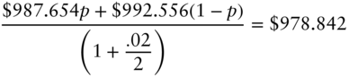
The price tree for $1,000 face value of a one‐year zero is depicted at the bottom right of Figure 7.1. The three prices on date 2 are all $1,000, which is the face value of the one‐year zero. The two prices on date 1 are found by discounting this certain $1,000 at the then‐prevailing six‐month rate. Hence, the date 1 upstate price is ![]() , or $987.654, and the date 1 downstate price is
, or $987.654, and the date 1 downstate price is ![]() , or $992.556. Finally, the date 0 price is computed using the given, date 0, one‐year rate of 2.15%:
, or $992.556. Finally, the date 0 price is computed using the given, date 0, one‐year rate of 2.15%: ![]() , or 978.842.
, or 978.842.
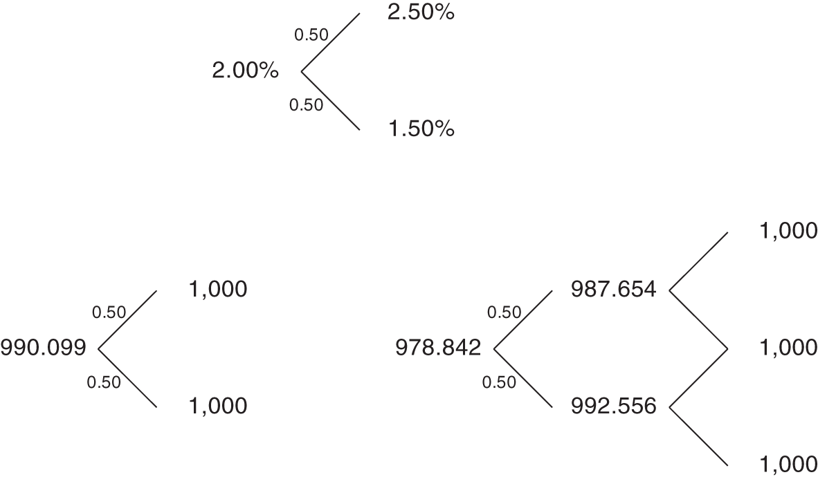
FIGURE 7.1 Pricing Six‐Month and One‐Year Zero Coupon Bonds with a Binomial Rate Tree.
The probabilities of moving up or down the tree may be used to compute average or expected values. As of date 0, the expected value of the one‐year zero price on date 1 is,
Discounting this expected value to date 0, at the date 0, six‐month rate gives an expected discounted value of,
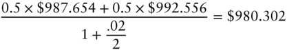
Note that the one‐year zero's expected discounted value of $980.302 is not equal to its market price of $978.842. These two numbers need not be equal, because investors do not price securities by expected discounted value. Over the next six months, the one‐year zero is a risky security, worth $987.654 half of the time and $992.556 the other half of the time, for an average or expected value of $990.105. If investors do not like this price uncertainty, they would prefer a security worth $990.105 on date 1 with certainty. More specifically, a security worth $990.105 with certainty after six months would sell for ![]() , or $980.302, as of date 0. By contrast, investors penalize the risky one‐year zero coupon bond with an average price of $990.105 in six months by pricing it today at $978.842. Chapters 8 and 9 elaborate further on investor risk aversion.
, or $980.302, as of date 0. By contrast, investors penalize the risky one‐year zero coupon bond with an average price of $990.105 in six months by pricing it today at $978.842. Chapters 8 and 9 elaborate further on investor risk aversion.
7.2 ARBITRAGE PRICING OF DERIVATIVES
This section prices an interest rate contingent claim or derivative, in particular, a call option that expires in six months to purchase $1,000 face value of a then six‐month zero at $990. Figure 7.2 starts the price tree for this call option based on the rates and prices in Figure 7.1. If on date 1 the six‐month rate is 2.50%, and a six‐month zero sells for $987.654, the right to buy that zero at $990 is worthless. On the other hand, if the six‐month rate is 1.50%, and the price of a six‐month zero is $992.556, then the right to buy the zero at $990 is worth ![]() , or $2.556. This description of the option's terminal payoffs emphasizes the contingent claim nature of the option: its value depends on interest rates through the value of an underlying bond.
, or $2.556. This description of the option's terminal payoffs emphasizes the contingent claim nature of the option: its value depends on interest rates through the value of an underlying bond.
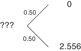
FIGURE 7.2 Pricing a 990 Six‐Month Call Option on a Six‐Month Zero Coupon Bond.
Chapter 1 showed that a security is priced by arbitrage by finding and pricing its replicating portfolio. In that context, because all bond cash flows are fixed or constant, the construction of the replicating portfolio is relatively simple. The present context is more difficult, because cash flows do depend on the level of rates, and the replicating portfolio must replicate the contingent claim for any possible interest rate scenario.
To price the call option of this section by arbitrage, construct a portfolio on date 0 of underlying securities, namely six‐month and one‐year zero coupon bonds, such that the portfolio is worth $0 in the upstate on date 1 and $2.556 in the downstate. Let ![]() and
and ![]() be the face values of six‐month and one‐year zeros in this replicating portfolio, respectively, and recall that the possible values of these bonds on date 1 are shown in Figure 7.1. These face amounts, therefore, must satisfy the following two equations,
be the face values of six‐month and one‐year zeros in this replicating portfolio, respectively, and recall that the possible values of these bonds on date 1 are shown in Figure 7.1. These face amounts, therefore, must satisfy the following two equations,
Equation (7.3) may be interpreted as follows. In the upstate, the value of the replicating portfolio's now maturing six‐month zero is its face value. The value of the once one‐year zeros, now six‐month zeros, is .987654 per dollar face value. Hence, the left‐hand side of Equation (7.3) denotes the value of the replicating portfolio in the upstate. This value must equal $0, the value of the option in the upstate. Similarly, Equation (7.4) sets the value of the replicating portfolio in the downstate equal to the value of the option in the downstate.
Solving Equations (7.3) and (7.4) gives ![]() and
and ![]() . In words, the option can be replicated by buying $521.4375 face value of one‐year zeros and shorting $515.0000 face amount of six‐month zeros on date 0. Therefore, by the law of one price, the price of the option equals the price of the replicating portfolio, which, using the bond prices given earlier, is equal to,
. In words, the option can be replicated by buying $521.4375 face value of one‐year zeros and shorting $515.0000 face amount of six‐month zeros on date 0. Therefore, by the law of one price, the price of the option equals the price of the replicating portfolio, which, using the bond prices given earlier, is equal to,

Recall that pricing based on the law of one price is enforced by arbitrage. If the price of the option were less than $0.504, arbitrageurs could buy the option, short the replicating portfolio, keep the difference, and have no future liabilities. Similarly, if the price of the option were greater than $0.504, arbitrageurs could short the option, buy the replicating portfolio, keep the difference, and, once again, have no future liabilities. Thus, ruling out profits from riskless arbitrage implies an option price of $0.504.
It is important to emphasize that the option cannot be priced by expected discounted value, which gives an option price of,
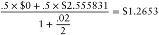
The true option price is lower, because investors dislike the risk of the call option and, as a result, will not pay as much as its expected discounted value. Put another way, the risk penalty implicit in the call option price is inherited from the risk penalty of the one‐year zero, that is, from the property that the price of the one‐year zero is less than its expected discounted value. Once again, the pricing of risk is discussed in the next two chapters. While this section illustrates arbitrage pricing with a call option, it should be clear that the framework can be used to price any security with cash flows that ultimately depend on the six‐month rate. For example, because the price of a five‐year bond over time depends on the evolution of the six‐month rate, an option on that five‐year bond can be priced in this framework as well.
A remarkable feature of arbitrage pricing is that the probabilities of up‐ and down‐moves never enter into the calculation of the arbitrage price. See Equations (7.3) through (7.5). The explanation for this somewhat surprising result follows from the principles of arbitrage. Arbitrage pricing requires that the value of the replicating portfolio be the same as the value of the option in both the up‐ and the down‐states. Therefore, the composition of the replicating portfolio is the same whether the probability of the upstate is 20%, 50%, or 80%. But if the composition of the portfolio does not depend directly on the probabilities, and if the prices of the securities in the portfolio are given, then the price of the replicating portfolio and the price of the option cannot depend directly on the probabilities either.
Despite the fact that the option price does not depend directly on the probabilities, these probabilities must have some impact on the option price. After all, as it becomes more and more likely that rates will rise to 2.50% and that bond prices will be low, the value of options to purchase bonds must fall. The resolution of this apparent paradox is that the option price depends indirectly on the probabilities through the price of the one‐year zero. Were the probability of an up move to increase suddenly, the current value of a one‐year zero would decline. And since the replicating portfolio is long one‐year zeros, the value of the option would decline as well. In summary, a derivative like an option depends on the probabilities only through current bond prices. Given bond prices, however, probabilities are not needed to derive prices determined by arbitrage.
7.3 RISK‐NEUTRAL PRICING
Risk‐neutral pricing is a technique that modifies an assumed interest rate process, like the one assumed at the start of this chapter, so that any contingent claim can be priced without having to construct and price its replicating portfolio. Because the technique requires that the original interest rate process be modified only once, and because this modification requires no more effort than pricing a single contingent claim by arbitrage, risk‐neutral pricing is an extremely efficient way to price many contingent claims under the same assumed rate process.
In the example of this chapter, the price of a one‐year zero does not equal its expected discounted value: its price is $978.842, computed from the given one‐year spot rate of 2.15%, while its expected discounted value is $980.302, as derived in Equation (7.2). The probabilities of 0.5 for the up‐ and down‐states are the assumed true or real‐world probabilities. But there are other probabilities, called risk‐neutral probabilities, which do cause the expected discounted value to equal the market price. To find these probabilities, let the risk‐neutral probabilities in the up‐ and down‐states be ![]() and
and ![]() , respectively. Then, solve the following equation,
, respectively. Then, solve the following equation,
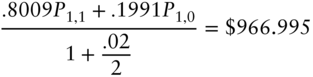
to find that ![]() . Hence, under the risk‐neutral probabilities of .8009 and .1991, the expected discounted value does equal the market price.
. Hence, under the risk‐neutral probabilities of .8009 and .1991, the expected discounted value does equal the market price.
Risk‐neutral probabilities can also be described in terms of the drift in interest rates. Under the true probabilities, there is a 50% chance that the six‐month rate rises from 2% to 2.50%, and a 50% chance that it falls from 2% to 1.50%. Hence, the expected change in the six‐month rate, or the drift of the six‐month rate, is zero. Under the risk‐neutral probabilities, there is an 80.09% chance of a 50‐basis point increase and a 19.91% chance of a 50‐basis point decrease, for an expected change of 30.09 basis points. Hence, the drift of the six‐month rate under these probabilities is 30.09 basis points.
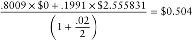
As pointed out in the previous section, the expected discounted value of the option payoff is $1.2653, while the arbitrage price is $0.504. But if expected discounted value were computed using the risk‐neutral probabilities, the resulting option value would equal its arbitrage price,
The fact that the arbitrage price of the option equals its expected discounted value under the risk‐neutral probabilities is not a coincidence. In general, to value contingent claims by risk‐neutral pricing, proceed as follows. First, find the risk‐neutral probabilities that equate the prices of the underlying securities to their expected discounted values. (In the simple example here, the only risky, underlying security is the one‐year zero.) Second, price the contingent claim by expected discounted value under these risk‐neutral probabilities. The remainder of this section describes intuitively why risk‐neutral pricing works. Since the argument is a bit complex, it is broken up into four steps:
- Given trees for the underlying securities, the price of a security that is priced by arbitrage does not depend on investors' risk preferences. The reasoning is as follows.
A security is priced by arbitrage if its cash flows can be replicated by some portfolio of underlying securities. Under the assumed process for interest rates in this chapter, the bond option is priced by arbitrage. By contrast, it is unlikely that a specific common stock can be priced by arbitrage, because no portfolio of underlying securities can mimic the idiosyncratic fluctuations of a single common stock's market value.
If a security is priced by arbitrage, and if everyone agrees on the price evolution of the underlying securities, then everyone agrees on the replicating portfolio. In the option example, both an extremely risk‐averse, retired investor and a professional gambler agree that a portfolio of $521.4375 face of one‐year zeros and ‐$515.0000 face of six‐month zeros replicates the option. And because they agree both on the composition of the replicating portfolio and on the prices of the underlying securities, they must also agree on the price of the option.
- Imagine an economy that has the same current bond prices and possible future values of the six‐month rate as the true economy. The imaginary economy is different, however, in that its investors are risk neutral. Unlike investors in the true economy, then, investors in the imaginary economy do not penalize securities for risk: they price securities by expected discounted value. In particular, under the probabilities in the imaginary economy, the expected discounted value of the one‐year zero equals its market price. But, by Equation (7.7), the expected discounted value of the one‐year zero does equal its market price under the risk‐neutral probabilities of .8009 and .1991. Hence, these risk‐neutral probabilities are the probabilities in the imaginary economy.
- The price of the option in the imaginary economy, like any other security in that economy, is computed by expected discounted value. Since the probability of the upstate in that economy is .8009, the price of the option in that economy is given by Equation (7.8) and is $0.504.
- Step 1 implies that, given the prices of the six‐month and one‐year zeros, as well as possible values of the six‐month rate, the price of an option does not depend on investor risk preferences. Therefore, because the real and imaginary economies have the same bond prices and the same possible values for the six‐month rate, the option price must be the same in both economies. In particular, the option price in the real economy must also equal $0.504. More generally, the price of a derivative in the real economy may be computed by expected discounted value under the risk‐neutral probabilities.
7.4 ARBITRAGE PRICING IN A MULTI‐PERIOD SETTING
Maintaining the binomial assumption, Figure 7.3 extends the tree from the previous section for another six months. This tree is called a recombining tree, because an up‐move followed by a down‐move, to the up–down state, lands in the same place as a down‐move followed by an up‐move, to the down–up state. Trees for which this is not the case are said to be nonrecombining. While nonrecombining trees might represent economically reasonable dynamics, they tend to be avoided as difficult or even impossible to implement. After six months there are two possible states, after one year there are four, and after ![]() semiannual periods there are
semiannual periods there are ![]() possibilities. A tree with enough semiannual steps to price 10‐year securities has, in its rightmost column alone, over 500,000 nodes, and to price 20‐year securities, over 500 billion. Furthermore, as discussed later in the chapter, it is often desirable to reduce the time interval between dates substantially. In short, even with modern computers, trees that grow this quickly are computationally unwieldy. This does not mean that the effects that seem to give rise to nonrecombining trees – like volatilities that change across states – cannot be modeled. It does mean, however, that such effects have to be implemented in more efficient ways.
possibilities. A tree with enough semiannual steps to price 10‐year securities has, in its rightmost column alone, over 500,000 nodes, and to price 20‐year securities, over 500 billion. Furthermore, as discussed later in the chapter, it is often desirable to reduce the time interval between dates substantially. In short, even with modern computers, trees that grow this quickly are computationally unwieldy. This does not mean that the effects that seem to give rise to nonrecombining trees – like volatilities that change across states – cannot be modeled. It does mean, however, that such effects have to be implemented in more efficient ways.
Returning to the recombining format, as trees grow it becomes convenient to develop a notation with which to refer to particular nodes. One convention is as follows. The dates, represented by columns of the tree, are numbered from left to right starting with 0. The states, represented by rows of the tree, are numbered from bottom to top, also starting from 0. For example, in Figure 7.3, the six‐month rate on date 2, state 0 is 1%. The six‐month rate on state 1 of date 1 is 2.50%.
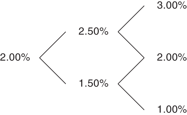
FIGURE 7.3 A Recombining Binomial Rate Tree.
Continuing where the option example left off, having derived the risk‐neutral tree for pricing a one‐year zero, the goal is to extend the tree to price a 1.5‐year zero assuming that the 1.5‐year spot rate is 2.25%. Ignoring the probabilities for a moment, several nodes of the 1.5‐year zero price tree can be written down immediately, as shown in Figure 7.4. On date 3, the zero with an original term of 1.5 years matures and is worth its face value of $1,000. On date 2, the value of the then six‐month zero equals its face value discounted for six months at the then‐prevailing spot rates of 3%, 2%, and 1%, in states 2, 1, and 0, respectively,
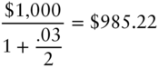
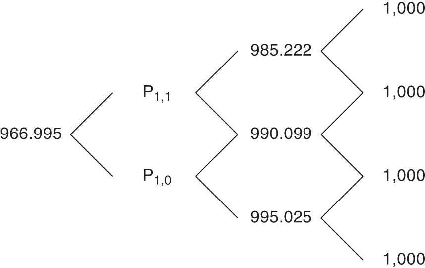
FIGURE 7.4 Price Tree for a 1.5‐Year Zero Coupon Bond.
Finally, on date 0, the 1.5‐year zero equals its face value discounted at the given, 1.5‐year spot rate,
The prices of the zero on date 1 in states 1 and 0 are denoted in Figure 7.4 by ![]() and
and ![]() , respectively. These one‐year zero prices are not known at this point.
, respectively. These one‐year zero prices are not known at this point.
The previous section showed that the risk‐neutral probability of an up‐move on date 0 is 0.8009. Letting ![]() be the risk‐neutral probability of an up‐move on date 1, and, for the purposes of this section, making the simplifying assumption that the probability of moving up from state 0 is the same as the probability of moving up from state 1, the resulting tree is shown in Figure 7.5.
be the risk‐neutral probability of an up‐move on date 1, and, for the purposes of this section, making the simplifying assumption that the probability of moving up from state 0 is the same as the probability of moving up from state 1, the resulting tree is shown in Figure 7.5.
By definition, the expected discounted value under risk‐neutral probabilities recovers market prices. With respect to the 1.5‐year zero price on date 0, this requires that,
And with respect to the prices of a then one‐year zero on date 1,
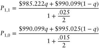
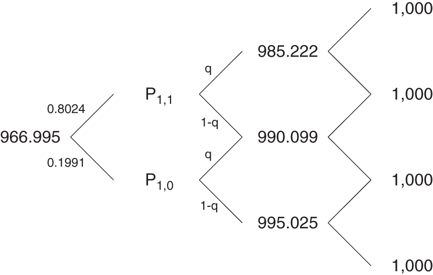
FIGURE 7.5 Price Tree for a 1.5‐Year Zero Coupon Bond, with Probabilities.
Substituting Equations (7.14) and (7.15) into Equation (7.13) results in a linear equation in the one unknown, ![]() , which can be solved to find that
, which can be solved to find that ![]() . Therefore, the risk‐neutral interest rate process is summarized by the tree in Figure 7.6. Furthermore, any contingent claim that depends on the six‐month rate in six months and in one year may be priced by computing its discounted expected value along this tree. An example is given in the next section.
. Therefore, the risk‐neutral interest rate process is summarized by the tree in Figure 7.6. Furthermore, any contingent claim that depends on the six‐month rate in six months and in one year may be priced by computing its discounted expected value along this tree. An example is given in the next section.
The difference between the true and risk‐neutral probabilities may once again be described in terms of drift. From dates 1 to 2, the drift under the true probabilities is zero. Under the risk‐neutral probabilities, the drift is computed from a 65.20% chance of a 50‐basis‐point increase in the six‐month rate and a 34.80% chance of a 50‐basis‐point decline in the rate. These numbers give a drift or expected change of 15.20 basis points.
Substituting ![]() back into Equations (7.14) and (7.15) completes the tree for the price of the 1.5‐year zero, which is shown in Figure 7.7. It follows immediately from this tree that the one‐year spot rate in six months may be either 2.5754% or 1.5754%, because,
back into Equations (7.14) and (7.15) completes the tree for the price of the 1.5‐year zero, which is shown in Figure 7.7. It follows immediately from this tree that the one‐year spot rate in six months may be either 2.5754% or 1.5754%, because,
(7.17)
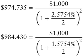
The fact that the possible values of the one‐year spot rate can be extracted from the tree is at first surprising. The starting point of the example is the date 0 values of the 0.5‐, 1‐, and 1.5‐year spot rates, along with assumptions about the evolution of the six‐month rate over the next years. But because this information, in combination with arbitrage or risk‐neutral arguments, is sufficient to determine the price tree of the 1.5‐year zero, it is also sufficient to determine the possible values of the one‐year spot rate in six months. Put another way, having specified initial spot rates and the evolution of the six‐month rate, a modeler may not make any further assumptions about the behavior of the one‐year rate.
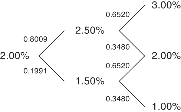
FIGURE 7.6 Risk‐Neutral Process for the Six‐Month Rate.
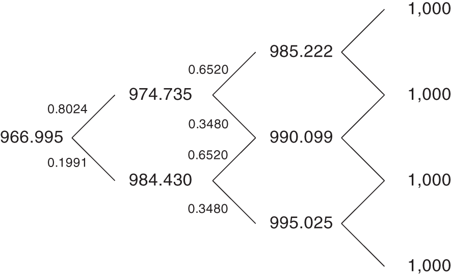
FIGURE 7.7 Final Price Tree for a 1.5‐Year Zero Coupon Bond, with Probabilities.
The six‐month rate process completely determines the one‐year rate process here, because the model presented has only one factor. Writing down a tree for the evolution of the six‐month rate alone implicitly assumes that prices of all fixed income securities can be determined by the evolution of that rate. A multi‐factor term structure model is presented in Chapter 9.
This section concludes with two additional observations about multi‐period settings. First, extending the tree to any number of dates requires assumptions about the future possible values of the short‐term rate and the calculation of risk‐neutral probabilities that recover a given set of bond prices. Second, the composition of replicating portfolios depends on date and state. For example, the replicating portfolio of a derivative as of date 0 is usually different from its replicating portfolio on date 1, state 0, and different again from its replicating portfolio on date 1, state 1. From a trading perspective, this means that replicating portfolios must be adjusted as time passes and as interest rates change. These adjustments are known as dynamic replication, in contrast to the static replication strategies of earlier chapters, like replicating a coupon bond with an unchanging portfolio of two other coupon bonds of the same maturity.
7.5 PRICING A CONSTANT‐MATURITY TREASURY SWAP
Equipped with the tree in Figure 7.7, this section prices a $1,000,000 stylized constant‐maturity Treasury (CMT) swap struck at 2%. This swap pays,
every six months until it matures, where ![]() is the semiannually compounded yield – of a predetermined maturity – on the payment date. This example prices a one‐year CMT swap on the six‐month yield, though, in practice, CMT swaps trade most commonly on the yields of the most liquid bonds, for example, on two‐, five‐ and 10‐year Treasury yields.
is the semiannually compounded yield – of a predetermined maturity – on the payment date. This example prices a one‐year CMT swap on the six‐month yield, though, in practice, CMT swaps trade most commonly on the yields of the most liquid bonds, for example, on two‐, five‐ and 10‐year Treasury yields.
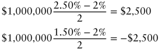
Because six‐month semiannually compounded yields equal six‐month spot rates, rates from the tree of the previous section can be substituted into Equation (7.18) to calculate the payoffs of the CMT swap. On date 1, the state 1 and state 0 payoffs are, respectively,
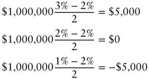
Similarly on date 2, the state 2, 1, and 0 payoffs are, respectively,
The possible values of the CMT swap at maturity, on date 2, are given by Equations (7.21) through (7.23). The possible values on date 1 are given by the expected discounted value of the date 2 payoffs under the risk‐neutral probabilities plus the date 1 payoffs given by (7.19) and (7.20). The resulting date 1 values in states 1 and 0 are, respectively,
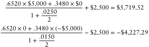
Finally, the value of the swap on date 0 is the expected discounted value, under the risk‐neutral probabilities, of the date‐1 payoffs, given by Equations (7.24) and (7.25),
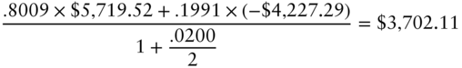
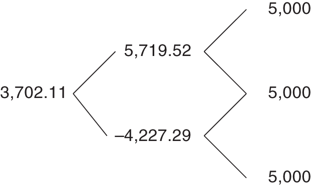
FIGURE 7.8 Price Tree for a Stylized CMT Swap.
The tree in Figure 7.8 summarizes the value of the stylized CMT swap over dates and states. A value of $3,702.11 for the CMT swap might seem surprising at first. After all, the cash flows of the CMT swap are zero at a rate of 2%, and 2% is, under the true probabilities, the average rate on each date. The explanation, of course, is that the risk‐neutral probabilities, not the true probabilities, determine the arbitrage price of the swap. The expected discounted value of the swap under the true probabilities can be computed by following the steps leading to Equations (7.24) through (7.26) but using the probability 0.5 for all up‐ and down‐moves. The result of these calculations does give a value close to zero, namely, −$6.07.
7.6 OPTION‐ADJUSTED SPREAD
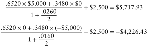
Option‐adjusted spread is a widely used measure of the relative value of a security, that is, of its market price relative to its model value. OAS is defined as the spread such that the market price of a security is recovered when that spread is added to discount rates in the model. To illustrate, say that the market price of the CMT swap in the previous section is $3,699.18, $2.92 less than the model price. In that case, the OAS of the CMT swap turns out to be 10 basis points. To see this, add 10 basis points to the discounting rates of 2.5% and 1.5% in Equations (7.24) and (7.25), respectively, to get new swap values of,
Note that, when calculating value with an OAS spread, rates are only shifted for the purpose of discounting. Rates are not shifted for the purposes of computing cash flows. In the CMT swap example, cash flows are still computed using Equations (7.19) through (7.23).
Completing the valuation with an OAS of 10 basis points, use the results of (7.27) and (7.28) and a discount rate of 2% plus the OAS spread of 10 basis points, or 2.10%, to obtain an initial CMT swap value of,
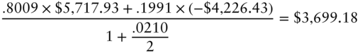
Hence, as claimed, discounting at the risk‐neutral rates plus an OAS of 10 basis points in the model recovers the given market price of $3,699.18. If a security's OAS is positive, its market price is less than its model price, which means that the security trades cheap. If the OAS is negative, the security trades rich.
Another perspective on the relative value implications of an OAS spread is the fact that the expected return of a security with an OAS, under the risk‐neutral process, is the short‐term rate plus the OAS per period. Very simply, discounting a security's expected value by a particular rate per period is equivalent to that security's earning that rate per period. In the example of the CMT swap, the expected return of the fairly priced swap under the risk‐neutral process over the six months from date 0 to date 1 is,

which is six months' worth of the initial rate of 2%. On the other hand, with an OAS of 10 basis points, the expected return of the cheap swap is,

which is six months' worth of the initial rate of 2% plus the OAS of 10 basis points, or half of 2.10%.
7.7 PROFIT AND LOSS ATTRIBUTION WITH AN OAS
Chapter 3 introduced profit and loss (P&L) attribution. This section gives a mathematical description of attribution in the context of term structure models and of securities that trade with an OAS. While the notation of this chapter is quite formal, the presentation remains intuitive.
By the definition of a one‐factor model, and by the definition of OAS, the market price of a security at time ![]() and a factor,
and a factor, ![]() , which is often a rate, can be written as
, which is often a rate, can be written as ![]() . Using a first‐order Taylor approximation, the change in the price of the security is,
. Using a first‐order Taylor approximation, the change in the price of the security is,
where ![]() gives the change in the price of the security for a change in
gives the change in the price of the security for a change in ![]() , holding
, holding ![]() and
and ![]() constant;
constant; ![]() gives the change in price for a change in
gives the change in price for a change in ![]() holding
holding ![]() and
and ![]() constant; and the same for
constant; and the same for ![]() . In words, Equation (7.32) breaks down the total change in price to components of change due to changes in
. In words, Equation (7.32) breaks down the total change in price to components of change due to changes in ![]() ,
, ![]() , and
, and ![]() .
.
Dividing both sides of Equation (7.32) by price and taking expectations,
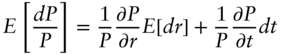
Note that ![]() is the change in price divided by price, or the percentage change in price. Because the OAS calculation assumes that OAS is constant over the life of the security, moving from (7.32) to (7.33) assumes that the expected change in the OAS is zero.
is the change in price divided by price, or the percentage change in price. Because the OAS calculation assumes that OAS is constant over the life of the security, moving from (7.32) to (7.33) assumes that the expected change in the OAS is zero.
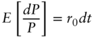
As mentioned in the previous section, if expectations are taken with respect to the risk‐neutral process, then, for any security priced according to the model,
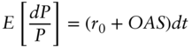
But Equation (7.34) does not apply to securities that are not priced according to the model, that is, to securities with an OAS not equal to zero. For these securities, by definition, the cash flows are discounted not at the short‐term rate, but at the short‐term rate plus the OAS. Equivalently, as argued in the previous section, the expected return under the risk‐neutral probabilities is not the short‐term rate, but the short‐term rate plus the OAS. Hence, the more general form of Equation (7.34) is,
Combining these pieces, substitute for ![]() from (7.33) and then for
from (7.33) and then for ![]() from (7.35) into Equation (7.32) and rearrange terms, which breaks down the return of a security into its component parts,
from (7.35) into Equation (7.32) and rearrange terms, which breaks down the return of a security into its component parts,
Finally, multiplying through by ![]() ,
,
In words, the return of a security or its P&L may be divided into a component due to the passage of time; a component due to changes in the factor; and a component due to the change in the OAS. In the language of Chapter 3, the terms on the right‐hand side of (7.37) represent, in order, carry–roll‐down, gains or losses from rate changes, and gains or losses from spread change.1 For models with predictive power, the OAS converges or trends to zero; that is, the security price converges or trends toward its fair value according to the model.
The decompositions of Equations (7.36) and (7.37) highlight the usefulness of OAS as a measure of value. If a model is correct, a long position in a cheap security earns superior returns in two ways. First, it earns the OAS over time intervals in which the security does not converge to its fair value. Second, it earns its sensitivity to OAS times any convergence of that OAS to zero.
The decompositions also provide a framework for relative value trading. When a cheap or rich security is identified, a relative value trader buys or sells the security and hedges out all interest rate or factor risk. Mathematically, ![]() . In that case, the expected return or P&L depends only on the short‐term rate, the OAS of the securities traded, and any OAS convergence. If the trader finances the trade at the short‐term rate, that is, borrows
. In that case, the expected return or P&L depends only on the short‐term rate, the OAS of the securities traded, and any OAS convergence. If the trader finances the trade at the short‐term rate, that is, borrows ![]() at rate
at rate ![]() to purchase the security, then the expected return is simply equal to the OAS plus any convergence return. If the hedge itself costs or generates funds, then the P&L also includes a return on those funds at the short‐term rate. If the hedging securities are not fairly priced relative to the model, but have an OAS of their own, then the P&L also includes an OAS on the hedge. Finally, Chapter 8 explains that bearing interest rate or factor risk may earn a risk premium, in which case there would be an additional term in Equations (7.34) through (7.37) that depends on the amount of factor risk borne. But, in the relative value context, where factor risk is hedged away, any risk premium terms cancel out, and the P&L of the trade is as described in this paragraph.
to purchase the security, then the expected return is simply equal to the OAS plus any convergence return. If the hedge itself costs or generates funds, then the P&L also includes a return on those funds at the short‐term rate. If the hedging securities are not fairly priced relative to the model, but have an OAS of their own, then the P&L also includes an OAS on the hedge. Finally, Chapter 8 explains that bearing interest rate or factor risk may earn a risk premium, in which case there would be an additional term in Equations (7.34) through (7.37) that depends on the amount of factor risk borne. But, in the relative value context, where factor risk is hedged away, any risk premium terms cancel out, and the P&L of the trade is as described in this paragraph.
7.8 REDUCING THE TIME STEP
This chapter has so far assumed that the time elapsed between dates of the tree is six months. The methodology outlined, however, adapts easily to any time step of ![]() years. For monthly time steps, for example,
years. For monthly time steps, for example, ![]() or .0833, and one‐month rather than six‐month interest rates appear on the tree. Furthermore, discounting is done over the appropriate time interval. If the rate of term
or .0833, and one‐month rather than six‐month interest rates appear on the tree. Furthermore, discounting is done over the appropriate time interval. If the rate of term ![]() is
is ![]() , then discounting means dividing by
, then discounting means dividing by ![]() . In the case of monthly time steps, discounting with a one‐month rate of 2% means dividing by
. In the case of monthly time steps, discounting with a one‐month rate of 2% means dividing by ![]() .
.
In practice there are two reasons to choose time steps smaller than six months. First, a security or portfolio of securities rarely makes all of its payments in even six‐month intervals from the starting date. Reducing the time step to a month, a week, or even a day can ensure that all cash flows are sufficiently close in time to some date in the tree. Second, assuming that the six‐month rate can take on only two values in six months, three values in one year, and so on, produces a tree that is too coarse for many practical pricing problems. Reducing the step size can fill the tree with enough rates to price contingent claims with sufficient accuracy.
While smaller time steps generate more realistic interest rate distributions, they require that more attention be paid to numerical issues, and they may make computations too slow for their intended uses. The choice of step size ultimately depends, therefore, on the problem at hand. When pricing a 30‐year callable bond, for example, a model with weekly or even monthly time steps may provide a realistic enough interest rate distribution to generate reliable prices. By contrast, pricing a one‐month bond option with any precision would require a much smaller time step. While the trees in this chapter assume that the step size is the same throughout the tree, this need not be the case. Sophisticated implementations of trees allow step size to vary across dates in order to achieve a balance between realism and computational concerns.
7.9 FIXED INCOME VERSUS EQUITY DERIVATIVES
The famous Black‐Scholes‐Merton (BSM) pricing analysis of stock options can be summarized as follows. Under the assumptions that the stock price evolves according to a particular random process and that the short‐term interest rate is constant, it is possible to form a portfolio of the underlying stock and short‐term bonds that replicates the option. Therefore, by arbitrage arguments, the price of the option equals the price of the replicating portfolio.
Consider applying this logic to price an option on a five‐year bond. The starting point might be an assumption about how the price of the five‐year bond evolves over time, but the task is considerably more complicated than for the price of a stock. First, the price of a bond converges to its face value at maturity, while the stock price has no similar constraint. Second, because of the maturity constraint, the volatility of a bond's price must decline as the bond approaches maturity. Hence, the simple assumption that the volatility of a stock is constant is not as appropriate for bonds. Third, because stock volatility is very large relative to short‐term rate volatility, it is often acceptable to assume that the short‐term interest rate is constant. By contrast, it seems inconsistent to assume that bond prices – which depend on interest rates – follow some random process, while assuming that the short‐term interest rate is constant.
These objections led researchers to make assumptions about the random evolution of the interest rate rather the bond price. In that way, bond prices naturally approach par, price volatilities naturally approach zero, and no interest rate is assumed to be constant. But this approach raises another set of questions. Which interest rate is assumed to evolve in a particular way? Assumptions about the five‐year spot rate, for example, are not sufficient for two reasons. First, five‐year coupon bond prices depend on shorter‐term spot rates as well. Second, an option on a particular five‐year bond soon depends on the prices of a bond that is no longer a five‐year bond, but a bond with slightly less time to maturity. Therefore, assumptions usually have to be made about the evolution of the entire term structure of interest rates to price bond options and other derivatives. This chapter shows that, in a one‐factor model, assumptions about the evolution of the short‐term rate are sufficient to model the evolution of the entire term structure.
In short, there are several arguments to move beyond BSM in the fixed income context. Nevertheless, for simplicity, practitioners do use versions of BSM to price and hedge several classes of fixed income derivatives. These methodologies are described at length in Chapter 16.
NOTE
- 1 For expositional simplicity no explicit coupon or other direct cash flows have been included in this discussion.