
APPENDIX TO CHAPTER 9
The Vasicek and Gauss+ Models
A9.1 THE VASICEK MODEL IN A BINOMIAL TREE
This section illustrates the implementation of the Vasicek model in a binomial tree. The parameters are ![]() ;
; ![]() ;
; ![]() ; and
; and ![]() . The step size is one year. The first stages of construction are shown in Figure A9.1. The starting short‐term rate, by definition is 2%. By a discrete time approximation to the dynamics of the risk‐neutral process in Equation (9.1) of the text, the expected short‐term rate after one year is,
. The step size is one year. The first stages of construction are shown in Figure A9.1. The starting short‐term rate, by definition is 2%. By a discrete time approximation to the dynamics of the risk‐neutral process in Equation (9.1) of the text, the expected short‐term rate after one year is,
Note that, if the time step were one month, instead of one year, the ![]() factor would be
factor would be ![]() instead of 1. In any case, adding a volatility of 0.95% up and down around the expectation from (A9.1) gives the date‐1 up‐ and down‐states in Figure A9.1.
instead of 1. In any case, adding a volatility of 0.95% up and down around the expectation from (A9.1) gives the date‐1 up‐ and down‐states in Figure A9.1.
Because of the mean reversion in the Vasicek model, computing the evolution of the short‐term rate over the next date is more complicated than the examples in Chapter 7. More specifically, because the drifts from the two states on date 1 are different from the drift from date 0, the tree does not necessarily recombine. One methodology for constructing a recombining tree is the following, though a full analysis of numerical issues is beyond the scope of this treatment.
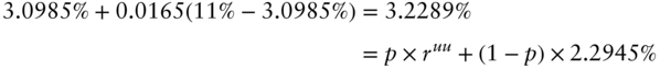
Given that the expected short‐term rate on date 1 is 2.1485%, as calculated in (A9.1), the expected short‐term rate on date 2 is,
which is the short‐term rate assigned to the date‐2, state 1 node of Figure A9.1.
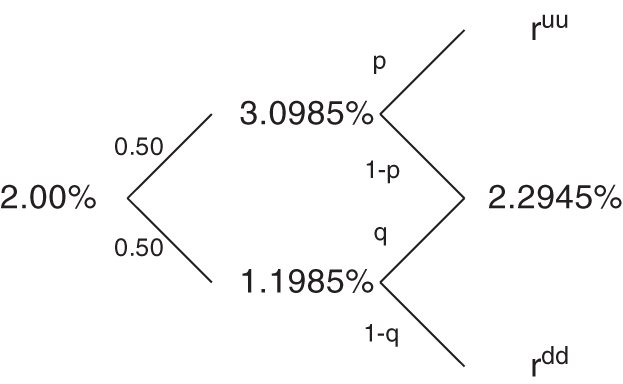
FIGURE A9.1 Binomial Tree Setup for Three Dates of the Vasicek Model.
The next stages of the construction are to find the missing rates and probabilities in Figure A9.1. From the date‐1 up‐state, the unknowns, ![]() and
and ![]() , must result in the drift and volatility specified by the model. Mathematically, the drift condition is,
, must result in the drift and volatility specified by the model. Mathematically, the drift condition is,
and the volatility condition is,
Solving Equations (A9.3) and (A9.4) simultaneously shows that ![]() and
and ![]() . These values are given in Figure A9.2 along with solutions to the analogous equations for
. These values are given in Figure A9.2 along with solutions to the analogous equations for ![]() and
and ![]() .1
.1
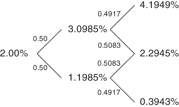
FIGURE A9.2 Binomial Tree Solution for Three Dates of the Vasicek Model.
A9.2 THE GAUSS+ MODEL
A9.2.1 Model Solution
Recall the dynamics of the short rate in cascade form presented in the text, where the cascade form means that each factor mean reverts to another factor, which mean reverts to another factor, in order of persistence. In order to solve the model (where “solving” means solving for the mapping from factors to forward rates), it will be convenient to work with the factors written in reduced form (where “reduced form” means that each factor mean reverts to a constant). After we have solved the model, we will write it back in cascade form in order to proceed to the estimation of its parameters. It will be convenient to partition the parameter vector ![]() in three blocks as
in three blocks as ![]() and
and ![]() and
and ![]() . In the reduced form, we have
. In the reduced form, we have ![]() and the relationship between the reduced form expression and cascade form expression of the factors is,
and the relationship between the reduced form expression and cascade form expression of the factors is,
where,
The dynamics of the reduced form factors are then given by,
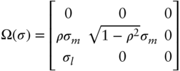
where for convenience we have appended a zero to the two‐dimensional random process ![]() and,
and,
Let ![]() denote the zero coupon bond price at time
denote the zero coupon bond price at time ![]() with time‐to‐expiry
with time‐to‐expiry ![]() . Taking the usual expectation of exponential of future short rate path conditional on the factors expressed in reduced form, one can show that,
. Taking the usual expectation of exponential of future short rate path conditional on the factors expressed in reduced form, one can show that,
where the yield of a zero coupon bond with maturity ![]() at time
at time ![]() is given by,
is given by,
where ![]() is a three‐dimensional vector with
is a three‐dimensional vector with ![]() for
for ![]() , and the term
, and the term ![]() can be written as,
can be written as,
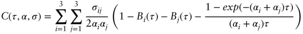
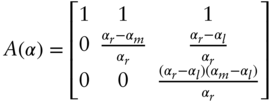
where ![]() stands for the
stands for the ![]() row and
row and ![]() column of matrix,
column of matrix, ![]() with,
with,

Mapping reduced form factors in (A9.10) to factors in cascade form, we finally have,
where 1 is a three‐dimensional column vector of ones and we have defined,
where ![]() where
where ![]() ,
, ![]() and
and ![]() represent the partial derivatives (a.k.a. loadings) of the changes of the zero coupon yield of maturity
represent the partial derivatives (a.k.a. loadings) of the changes of the zero coupon yield of maturity ![]() on the short, medium and long rate factors. A similar representation for the (continuously compounded) forward rate of tenor
on the short, medium and long rate factors. A similar representation for the (continuously compounded) forward rate of tenor ![]() as an affine function of the factors in cascade form can be obtained as follows,
as an affine function of the factors in cascade form can be obtained as follows,
where,
Expression (A9.15) can be interpreted as follows: The time ![]() forward rate with maturity
forward rate with maturity ![]() and tenor
and tenor ![]() can be decomposed into a component that represents the risk‐neutral expectation of the
can be decomposed into a component that represents the risk‐neutral expectation of the ![]() maturity yield prevailing at time
maturity yield prevailing at time ![]() (first two terms of the right‐hand side) minus a component that represents the convexity advantage of receiving (i.e., being long) rates (third term of the right‐hand side). The first on the right‐hand side component can be shown to be null for
(first two terms of the right‐hand side) minus a component that represents the convexity advantage of receiving (i.e., being long) rates (third term of the right‐hand side). The first on the right‐hand side component can be shown to be null for ![]() and converges to
and converges to ![]() as
as ![]() grows toward infinity. For maturities between zero and infinity, the risk‐neutral expectation of the zero yield prevailing at that maturity will depend on the value that the factors take at time
grows toward infinity. For maturities between zero and infinity, the risk‐neutral expectation of the zero yield prevailing at that maturity will depend on the value that the factors take at time ![]() , namely,
, namely, ![]() , and this is what the second term on the right‐hand side captures. We can also think of the sum of the first two components on the right‐hand side as the fair futures rate at time
, and this is what the second term on the right‐hand side captures. We can also think of the sum of the first two components on the right‐hand side as the fair futures rate at time ![]() for a mark‐to‐market futures contract on the zero coupon yield that will prevail at time
for a mark‐to‐market futures contract on the zero coupon yield that will prevail at time ![]() . The shape of the slopes
. The shape of the slopes ![]() , evaluated at estimated parameter values, are displayed in Figure 9.7.
, evaluated at estimated parameter values, are displayed in Figure 9.7.
The last term on the right‐hand side of (A9.15) is null for ![]() and grows at speed equal to the square of maturity
and grows at speed equal to the square of maturity ![]() . This convexity term drives a wedge between the futures rate and the forward rate. Imagine that an investor can bet on the yield that will prevail at time
. This convexity term drives a wedge between the futures rate and the forward rate. Imagine that an investor can bet on the yield that will prevail at time ![]() in two different contracts: the first is a daily‐settled futures contract. Any increase (decrease) in the market expected future rate will be paid (received) today by the long (short) investor. The second is a standard forward contract. Any increase (decrease) in the market expected future rate will be paid (received) by the long (short) investor not today, but at time
in two different contracts: the first is a daily‐settled futures contract. Any increase (decrease) in the market expected future rate will be paid (received) today by the long (short) investor. The second is a standard forward contract. Any increase (decrease) in the market expected future rate will be paid (received) by the long (short) investor not today, but at time ![]() . Now, if the futures rate and the forward rate were equal, the long investor would be at an advantage in transacting via the forward contract rather than the futures contract: when the market future rate expectation increases (decreases) their future losses (gains) will be discounted to today at a relatively higher (lower) rate, hence yielding a relatively smaller (larger) present value loss (gain). Therefore, to prevent an arbitrage between forward and futures rates, today's forward rate should be somewhat lower than today's futures rate. The difference between the two is what we call the convexity correction or convexity advantage term, that is, the last term on the right hand side.
. Now, if the futures rate and the forward rate were equal, the long investor would be at an advantage in transacting via the forward contract rather than the futures contract: when the market future rate expectation increases (decreases) their future losses (gains) will be discounted to today at a relatively higher (lower) rate, hence yielding a relatively smaller (larger) present value loss (gain). Therefore, to prevent an arbitrage between forward and futures rates, today's forward rate should be somewhat lower than today's futures rate. The difference between the two is what we call the convexity correction or convexity advantage term, that is, the last term on the right hand side.
A9.2.2 A Practical Estimation Method
There exists a large literature on estimating gaussian term structure models, of which the Gauss+ model is a particular case. The methods typically rely on maximum‐likelihood estimation procedures which are not easy to implement in general. In the next section we discuss a procedure that is fast and intuitive for the purpose of finding reasonable values for the Gauss+ parameter vector ![]() . Given this parameter vector, and for any time
. Given this parameter vector, and for any time ![]() , we will then extract the factors
, we will then extract the factors ![]() in order to have the model zero yields be close to the market zero yields. The short rate
in order to have the model zero yields be close to the market zero yields. The short rate ![]() will not need to be filtered because it will be set equal to the observed short policy rate.
will not need to be filtered because it will be set equal to the observed short policy rate.
In order to estimate parameters ![]() , we first obtain a time series of zero coupon bond prices (discount factors) at different maturities. These can be obtained by using an external curve construction bootstrap method using bonds or par swap rates. For the purpose of fitting the Gauss+ model, it does not matter whether these discount factors come from a swap curve (index or discount curves) or from a bond curve. Here we will use the time series of zero coupon bonds published by the New York Fed, which is based on applying the well‐known Nelson‐Siegel‐Svensson smooth curve construction procedure to US Treasury notes and bonds.2
, we first obtain a time series of zero coupon bond prices (discount factors) at different maturities. These can be obtained by using an external curve construction bootstrap method using bonds or par swap rates. For the purpose of fitting the Gauss+ model, it does not matter whether these discount factors come from a swap curve (index or discount curves) or from a bond curve. Here we will use the time series of zero coupon bonds published by the New York Fed, which is based on applying the well‐known Nelson‐Siegel‐Svensson smooth curve construction procedure to US Treasury notes and bonds.2
There is always a trade‐off when it comes to selecting the sample for the estimation of the model. Longer samples will lead to more robust estimates in a statistical sense but will also reflect different market conditions from the ones in which we intend to use the model. We have found that, in practice, a good compromise is to use a sample size of eight years and a decay factor of 0.8. (This means that in the loss‐functions associated with the optimization problems that follow we will give a weight of 1 to the last observation, a weight of 0.8 to an observation that is one year old relative to the last observation, a weight of 0.64 to an observation that is two years old relative to the last observation, and so forth.) Our sample thus begins on January 5, 2014, and ends on January 21, 2022.
While the Gauss+ model involves three factors, only two are genuine factors as we will equal the short rate to a given observed short rate, which tends to change at predictable dates. For this reason, we will take the short rate ![]() to be the fed funds target. While taking the general collateral repo rate would be closer to the actual overnight funding rate for US Treasury bonds, this series also exhibits spikes that reflect circumstantial funding conditions and are generally unrelated to monetary policy, and hence unrelated to expectations of future paths of the short rate.
to be the fed funds target. While taking the general collateral repo rate would be closer to the actual overnight funding rate for US Treasury bonds, this series also exhibits spikes that reflect circumstantial funding conditions and are generally unrelated to monetary policy, and hence unrelated to expectations of future paths of the short rate.
In what follows we will denote by ![]() the
the ![]() matrix of observed zero coupon yields for
matrix of observed zero coupon yields for ![]() periods and
periods and ![]() maturities, and by
maturities, and by ![]() the vector of
the vector of ![]() maturity yields observed at time
maturity yields observed at time ![]() . Similarly, we will denote by
. Similarly, we will denote by ![]() the vector of model implied zero coupon yields for
the vector of model implied zero coupon yields for ![]() periods and
periods and ![]() maturities.
maturities. ![]() is a function of
is a function of ![]() , the
, the ![]() vector of factors in cascade form. In addition, let and
vector of factors in cascade form. In addition, let and ![]() , as described in (A9.13), stand for the vector of yields for the
, as described in (A9.13), stand for the vector of yields for the ![]() maturities as a function of the cascade form factors at time
maturities as a function of the cascade form factors at time ![]() , namely,
, namely, ![]() . Finally, let
. Finally, let ![]() stand for the yield of maturity
stand for the yield of maturity ![]() at time
at time ![]() , as a function of the factors and the parameter vector
, as a function of the factors and the parameter vector ![]() .
.
Estimation involves one step for data preparation, and three steps for parameter optimization. Data preparation consists of netting the effect of the (observed) short rate factor from the observed zero coupon yields. This works as follows. Take a candidate parameter value for ![]() . Then, given the structure of
. Then, given the structure of ![]() , subtract
, subtract ![]() from both sides of (A9.13). With an abuse of notation, we will denominate
from both sides of (A9.13). With an abuse of notation, we will denominate ![]() the zero coupon yield netted out of the short rate, and we will drop the short rate
the zero coupon yield netted out of the short rate, and we will drop the short rate ![]() from the vector of factors in cascade form, so from now on we have
from the vector of factors in cascade form, so from now on we have ![]() . Incidentally, one could show that
. Incidentally, one could show that ![]() depends only on parameter
depends only on parameter ![]() .
.
The next step consists of inverting (A9.13) and expressing the factors ![]() as a linear function of the observed two‐ and 10‐year yields (henceforth 2y and 10y). We will assume that the yields of these two maturities are priced exactly by the model, unlike other maturities. Denote these benchmark yields at time
as a linear function of the observed two‐ and 10‐year yields (henceforth 2y and 10y). We will assume that the yields of these two maturities are priced exactly by the model, unlike other maturities. Denote these benchmark yields at time ![]() as
as ![]() . We can then invert (A9.13) for the 2y and 10y maturity and express the factors in cascade form as linear functions of the vector of benchmark yields. Then we replace the resulting expression for the factors in (A9.13). Finally, write the resulting expression of benchmark yields as a function of factors, in changes,
. We can then invert (A9.13) for the 2y and 10y maturity and express the factors in cascade form as linear functions of the vector of benchmark yields. Then we replace the resulting expression for the factors in (A9.13). Finally, write the resulting expression of benchmark yields as a function of factors, in changes,
where ![]() stands for a matrix formed by the vectors (A9.14) corresponding to maturities
stands for a matrix formed by the vectors (A9.14) corresponding to maturities ![]() , and dropping the column. Now, solving for
, and dropping the column. Now, solving for ![]() and plugging the resulting expression into equation (A9.13) written in changes, we obtain a linear expression relating the yield changes at any maturity to the yield changes of the two benchmark maturities, where the slopes are a nonlinear function of just the parameter
and plugging the resulting expression into equation (A9.13) written in changes, we obtain a linear expression relating the yield changes at any maturity to the yield changes of the two benchmark maturities, where the slopes are a nonlinear function of just the parameter ![]() ,
,
we can then compute an estimate for ![]() by solving,
by solving,
where ![]() stands for the L2 norm and
stands for the L2 norm and ![]() is the ordinary least square estimate of regressing
is the ordinary least square estimate of regressing ![]() onto
onto ![]() , namely,
, namely,
Figure 9.5 in the text shows the estimated OLS parameters of regressing yield changes at different maturities on the changes in the two‐ and 10‐year yield. It also shows the values of the model slopes ![]() , evaluated at the optimal solution of (A9.20). The parameter
, evaluated at the optimal solution of (A9.20). The parameter ![]() allows one to examine the impact of a change in the factors
allows one to examine the impact of a change in the factors ![]() on the instantaneous forward rates and yields. This allows a clear interpretation of each of the factors: the medium rate
on the instantaneous forward rates and yields. This allows a clear interpretation of each of the factors: the medium rate ![]() has maximum impact around the 2y to 3y maturities; hence it can be interpreted as a monetary policy factor (as has been argued in the text). On the other hand, the long factor exhibits maximum impact around the 7y forward maturity (and 15y for zero yield maturity).
has maximum impact around the 2y to 3y maturities; hence it can be interpreted as a monetary policy factor (as has been argued in the text). On the other hand, the long factor exhibits maximum impact around the 7y forward maturity (and 15y for zero yield maturity).
Armed with the estimated parameter ![]() that solves (A9.20), we proceed to estimate the vector
that solves (A9.20), we proceed to estimate the vector ![]() that minimizes the distance between model implied yield volatilities and realized volatilities of constant maturity yields by solving,
that minimizes the distance between model implied yield volatilities and realized volatilities of constant maturity yields by solving,
where ![]() is a
is a ![]() vector of yield changes for all maturities. Figure 9.6 in the text shows the fitted zero yield volatilities, versus the volatilities computed directly from observed, constant maturity yield changes.
vector of yield changes for all maturities. Figure 9.6 in the text shows the fitted zero yield volatilities, versus the volatilities computed directly from observed, constant maturity yield changes.
Finally, using ![]() that solves (A9.20) and
that solves (A9.20) and ![]() that solves (A9.22), we determine the parameter
that solves (A9.22), we determine the parameter ![]() by minimizing the sum of squares of yield fitting errors, namely,
by minimizing the sum of squares of yield fitting errors, namely,
where ![]() is the vector of model yields for all maturities, at time
is the vector of model yields for all maturities, at time ![]() . The estimated parameters are shown in Table 9.1 in the text.
. The estimated parameters are shown in Table 9.1 in the text.
Once the parameter vector ![]() has been estimated, we can solve for the factors
has been estimated, we can solve for the factors ![]() to ensure that the model fits exactly the two‐ and 10‐year forward rates (with tenor one year) on each date. (Filtering methods such as least‐squares or Kalman filtering could be employed to extract fitted factors, but we find exact fitting of two points in the curve is preferable in practical trading applications.) We show the fitted factors in Figure 9.8 in the text, along with the 2y forward rate.3
to ensure that the model fits exactly the two‐ and 10‐year forward rates (with tenor one year) on each date. (Filtering methods such as least‐squares or Kalman filtering could be employed to extract fitted factors, but we find exact fitting of two points in the curve is preferable in practical trading applications.) We show the fitted factors in Figure 9.8 in the text, along with the 2y forward rate.3
Note that in the text we plot the affine function of ![]() ,
, ![]() below rather than
below rather than ![]() itself, so that we can interpret the derived long factor as an approximation of the expectation of what the short rate will be in 10 years' time. This is necessary because the extreme persistence (or large half‐life, or low mean‐reversion parameter) of the factor
itself, so that we can interpret the derived long factor as an approximation of the expectation of what the short rate will be in 10 years' time. This is necessary because the extreme persistence (or large half‐life, or low mean‐reversion parameter) of the factor ![]() makes the interpretation of the fitted level of
makes the interpretation of the fitted level of ![]() less intuitive. As you can see, the long factor closely tracks the 10y forward rate from before (the difference between the two is explained by the convexity correction adjustment),
less intuitive. As you can see, the long factor closely tracks the 10y forward rate from before (the difference between the two is explained by the convexity correction adjustment),
The time series properties of the model can be described by graphing its fitted factors over time. As mentioned already, the short‐term rate is set each day to the fed funds target rate, and the medium‐ and long‐term factors are set so as to match the model and market two and 10 years forward. Figure 9.8 in the text graphs these empirically recovered market factors from January 2007 to January 2022.4
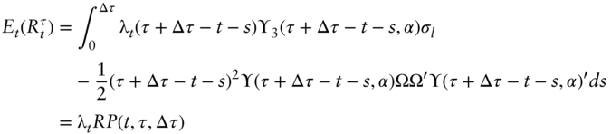
A9.2.3 Implied Risk Premia Calculation
Denote by ![]() the price at time
the price at time ![]() of a zero coupon bond that matures at time
of a zero coupon bond that matures at time ![]() and let
and let ![]() . Note that here
. Note that here ![]() stands for a fixed date in the future, and not a date interval.
stands for a fixed date in the future, and not a date interval.
We will assume henceforth that only the risk of the long factor is priced. This is reasonable for the application we have in mind, which will involve extracting expectations about the 10‐year maturity and, at that maturity, the loadings of the forward relative to the short and medium rate are negligible. Now, applying Ito's lemma to the zero coupon bond price as an exponential affine function of the cascade form factors (A9.9) using (A9.13), and passing to the true measure, we can write the dynamics of the instantaneous return of a zero coupon bond as follows,

where the loadings vector ![]() was defined in (A9.14), and
was defined in (A9.14), and ![]() stands for its last element, i.e., the loading of a zero coupon yield with maturity
stands for its last element, i.e., the loading of a zero coupon yield with maturity ![]() on the long rate factor. Also,
on the long rate factor. Also, ![]() was defined in (A9.8) and
was defined in (A9.8) and ![]() stands for the Wiener process under the true measure.
stands for the Wiener process under the true measure.
The term multiplying ![]() on the right‐hand side of (A9.25) has a clear interpretation: the expected return at time
on the right‐hand side of (A9.25) has a clear interpretation: the expected return at time ![]() of holding
of holding ![]() maturity zero coupon bond from time
maturity zero coupon bond from time ![]() to time
to time ![]() is equal to the riskless rate prevailing at time
is equal to the riskless rate prevailing at time ![]() , plus a risk‐premium term that is equal to the duration of the zero coupon bond (its maturity) times the loading of the yield of a zero coupon bond with maturity
, plus a risk‐premium term that is equal to the duration of the zero coupon bond (its maturity) times the loading of the yield of a zero coupon bond with maturity ![]() , times the volatility of the long rate, times the price of risk prevailing at time t, namely,
, times the volatility of the long rate, times the price of risk prevailing at time t, namely, ![]() . We will assume that the price of risk does change over time. We will not specify its dynamics, but we will assume that
. We will assume that the price of risk does change over time. We will not specify its dynamics, but we will assume that ![]() is a very persistent process, so that
is a very persistent process, so that ![]() for
for ![]() , i.e. one price of risk next‐year is expected to be equal to this year's. If we changed measure to the risk‐neutral measure, this term would disappear from the right‐hand side of (A9.25), that is, the expected instantaneous return of our zero coupon bond would equal the riskless rate.
, i.e. one price of risk next‐year is expected to be equal to this year's. If we changed measure to the risk‐neutral measure, this term would disappear from the right‐hand side of (A9.25), that is, the expected instantaneous return of our zero coupon bond would equal the riskless rate.
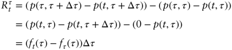
Recall as well the definition of the forward rate at time ![]() with maturity
with maturity ![]() and tenor
and tenor ![]() :
: ![]() – we will omit the tenor as an explicitly argument of
– we will omit the tenor as an explicitly argument of ![]() . Now, consider the following strategy: At time
. Now, consider the following strategy: At time ![]() , buy one zero coupon bond with maturity
, buy one zero coupon bond with maturity ![]() , and simultaneously sell one zero coupon bond with maturity
, and simultaneously sell one zero coupon bond with maturity ![]() . First, we claim that the return of this strategy is equal to the forward rate with tenor
. First, we claim that the return of this strategy is equal to the forward rate with tenor ![]() prevailing at time
prevailing at time ![]() , minus the
, minus the ![]() maturity yield prevailing at time
maturity yield prevailing at time ![]() . To see this, denote by
. To see this, denote by ![]() the cumulative realized return between time
the cumulative realized return between time ![]() and time
and time ![]() . We then have,
. We then have,
where ![]() is equal to the zero coupon yield with maturity
is equal to the zero coupon yield with maturity ![]() prevailing at time
prevailing at time ![]() which, for a sufficiently small
which, for a sufficiently small ![]() , approximately equals the spot rate prevailing at time
, approximately equals the spot rate prevailing at time ![]() . Hence, the expected return (under the true measure) of this strategy at time
. Hence, the expected return (under the true measure) of this strategy at time ![]() is equal to the forward rate at time
is equal to the forward rate at time ![]() , minus the expected short rate at time
, minus the expected short rate at time ![]() . Let's keep this result aside for a moment.
. Let's keep this result aside for a moment.
We will now compute the expected return of this strategy (again, under the true measure). Note that the expected return of the long and short side cancel out for entire the holding period except for the segment ![]() and
and ![]() , because in the model the risk premia depends on time to maturity only. Applying Ito's lemma to (A9.25), canceling the short rate, integrating and taking expectations, and dismissing the contribution of the segments
, because in the model the risk premia depends on time to maturity only. Applying Ito's lemma to (A9.25), canceling the short rate, integrating and taking expectations, and dismissing the contribution of the segments ![]() because only the long factor is priced, we get,
because only the long factor is priced, we get,
Note that the expected risk premium (A9.27) is the product of the yet unknown ![]() and an amount of risk term
and an amount of risk term ![]() that can be easily computed. As we mention in the text, in order to imply
that can be easily computed. As we mention in the text, in order to imply ![]() from the observed forward rates and the parameters of the model, we will assume that there is a maturity
from the observed forward rates and the parameters of the model, we will assume that there is a maturity ![]() such that the (true) expectation of what the short rate will be at maturity
such that the (true) expectation of what the short rate will be at maturity ![]() is equal to the (true) expectation of the short rate will be at any maturity
is equal to the (true) expectation of the short rate will be at any maturity ![]() . With this assumption, we can specialize this reasoning to two long maturities
. With this assumption, we can specialize this reasoning to two long maturities ![]() , subtract the resulting equations and solve for the price of risk
, subtract the resulting equations and solve for the price of risk ![]() as follows,
as follows,
Armed with an estimate for ![]() , we can then take expectations on both sides of the equation (A9.26) at maturity
, we can then take expectations on both sides of the equation (A9.26) at maturity ![]() and use (A9.27) to solve for the expected rate for a long enough maturity
and use (A9.27) to solve for the expected rate for a long enough maturity ![]() . We finally get,
. We finally get,
To get an intuition for (A9.29), say that the price of risk ![]() that we solved before is 0.09. The loading of the 10‐year zero coupon bond yield on the long factor is 0.7, and the volatility of the long factor is about 100 basis points, then the 10‐year risk premium would be approximately
that we solved before is 0.09. The loading of the 10‐year zero coupon bond yield on the long factor is 0.7, and the volatility of the long factor is about 100 basis points, then the 10‐year risk premium would be approximately ![]() bps. The convexity advantage term for the 10‐year rate is about 24bps. These numbers are very close to the ones obtained by evaluating the model at estimated parameters, and 0.09 is the average price of risk in the sample.5 If we assume that the 10‐year forward rate is
bps. The convexity advantage term for the 10‐year rate is about 24bps. These numbers are very close to the ones obtained by evaluating the model at estimated parameters, and 0.09 is the average price of risk in the sample.5 If we assume that the 10‐year forward rate is ![]() , the implied expected one‐year rate, nine years rate under the true measure would then be
, the implied expected one‐year rate, nine years rate under the true measure would then be ![]()
We computed the price of risk in the manner described already for using the 14‐ and 15‐year forwards to extract ![]() for every day in our sample, and then using this estimate to imply the expectation of the 10‐year rate using the 10‐year forward rate. Results are not sensitive to using other, longer maturities.
for every day in our sample, and then using this estimate to imply the expectation of the 10‐year rate using the 10‐year forward rate. Results are not sensitive to using other, longer maturities.
The implied 10‐year rate expectation computed in this manner is plotted in the text against an estimate of the long run expected short rate obtained outside the model, just by just adding the real rate forecast produced by the Cleveland Fed, to a measure of long run inflation, which we took as the average of the 10‐year inflation rate forecast produced by the Cleveland Fed, the 10‐year forecast produced by the ATSIX model of the Philadelphia Fed, and an estimate of trend inflation obtained with a simple exponential moving average rule with a decay parameter of 0.987, a value used elsewhere in the literature.6 Other procedures to assess long rate expectations are possible (for example, the Survey of Market Participants conducted by the New York Fed several times a year, or the long‐standing Bluechip Financial Forecast survey).
NOTES
- 1 The values of
 and
and  are the same to four decimal places but are not identically equal.
 - 2 See Gürkaynak, R., Sack, B., and Wright, J. (2006), “The US Treasury Yield Curve: 1961 to the Present,” and https://www.federalreserve.gov/data/nominal‐yield‐curve.html
- 3 While the sample we used for parameter estimation starts in January 2014, we expanded the period for which we extract the filtered factors backward to create Figure 9.8 – holding the estimated parameters constant – in order to facilitate interpretation.
- 4 The model is estimated using data from January 2014, but the resulting parameters are used to extract model factors back through 2007. Also, instead of the long‐term factor itself, the figure graphs the long‐term factor shifted forward 10 years. This allows the series to be more easily interpreted as an approximation for expectations of the short‐term rate in 10 years.
- 5 This value may look low for the usual estimates of Sharpe ratio obtained for risky assets. Note, however, that bonds prices have been negatively correlated with risky assets for the last decades, and thus a lower price of interest rate risk relative to risky asset in positive supply (e.g., the stock market), even negative at times, should be expected.
- 6 See for example, Cieslak, A., and Povala, P. (2015), “Expected Returns in Treasury Bonds,” Review of Financial Studies 28(10).