
APPENDIX TO CHAPTER 11
Note and Bond Futures
A11.1 FORWARD DROP APPROXIMATELY EQUALS CASH CARRY
Define the following notation, all for 100 face amount of a bond:
 : flat price for spot settlement
 : annual coupon payment
 : number of days from spot settlement to the coupon payment date
 : number of days from the coupon payment date to forward settlement
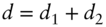 : number of days from spot to forward settlement
 : accrued interest as of spot and forward settlements, respectively
 : repo rate from spot to forward settlement
 : flat price for forward settlement
With this notation, the forward price of the bond, based on the discussion in the text, can be written as,
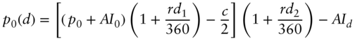
Equation (A11.2) follows from Equation (A11.1) by dropping terms that are small, because they represent interest‐on‐interest. In particular, the following approximations are made: ![]() ; and
; and ![]() .
.
A11.2 FORWARD VERSUS FUTURES PRICES IN A TERM STRUCTURE MODEL
This section highlights the differences between pricing forward and futures contracts in a term structure model. To focus on this difference, it is assumed here that the futures contract has one delivery date and one deliverable bond and that its conversion factor is one. Section A11.4 discusses the pricing of delivery options in a term structure model. Also, for simplicity, it is assumed here that there are no intermediate coupon dates between the spot and forward settlement dates.
Using the methodology of Chapter 7, begin with a recombining, binomial tree with three dates, labeled 0, 1, and 2, where the forward and futures contracts expire on date 2. Set the following notation:
 ,
,  , and
, and  : the initial one‐period rate, and the one‐period rates on date 1, in the up and down states, respectively.
 ,
,  ,
,  , and
, and  : the initial full price of the underlying bond, and the date‐2 full prices in the “up–up,” “up–down,” and “down–down” states, respectively.
 ,
,  ,
,  , and
, and  : flat prices at the indicated dates and states.
 : the initial full forward price.
 : the initial flat forward price.
 ,
,  ,
,  : the initial futures price, and the date‐1 futures prices in the up and down states, respectively.
 ,
,  : the risk‐neutral transition probabilities on all dates to move up and down from the current state, respectively.
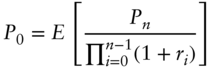
By the definition of a risk‐neutral tree, the initial price of the bond can be computed as,
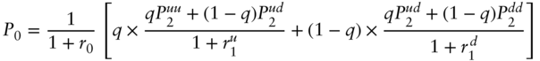
or, rearranging terms,
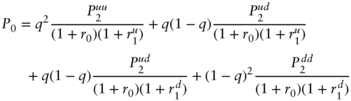
Each term of Equation (A11.4) is the probability of a particular path through the tree times the discounted value of the bond price at the end of that path, where discounting is done using the short‐term rates along the path. Taking all terms together, therefore, ![]() is the expected discounted bond price. More generally, then, letting
is the expected discounted bond price. More generally, then, letting ![]() be the number of periods,
be the number of periods, ![]() the random full price of the bond at period
the random full price of the bond at period ![]() , and
, and ![]() the random short‐term rate over period
the random short‐term rate over period ![]() to
to ![]() ,
,
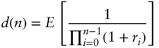
The discount factor to period ![]() ,
, ![]() , is just a special case of (A11.5) when the terminal price equals one in all states. Hence,
, is just a special case of (A11.5) when the terminal price equals one in all states. Hence,
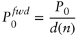
Following the discussion in the text, the forward full price of the bond is just the future value, to the forward delivery date, of the full spot price of the bond. Therefore, using Equations (A11.5) and (A11.6),
Turning to the futures price, start again with the recombining, risk‐neutral binomial tree. At expiration on date 2, the futures price equals the flat bond price. (At contract expiration, the bond is delivered at the futures price plus accrued interest.) In the up state of date 1, the futures price is ![]() , which means that the daily settlement payment for a long position of one contract on date 2 is
, which means that the daily settlement payment for a long position of one contract on date 2 is ![]() in the up‐up state and
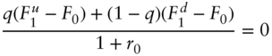
in the up‐up state and ![]() in the up‐down state. But because the value of a futures contract initiated at any date is zero, the expected discounted value of the daily settlement payments from the date 1 up state must be zero. Hence,
in the up‐down state. But because the value of a futures contract initiated at any date is zero, the expected discounted value of the daily settlement payments from the date 1 up state must be zero. Hence,
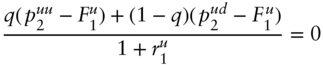
And, solving for the futures price,
Analogously, the futures price in the date 1 down state is,
On date 0, the futures price is ![]() , and the expected discounted value of the date 1 settlement payment must be zero. Hence,
, and the expected discounted value of the date 1 settlement payment must be zero. Hence,
Or,
Finally, substituting Equations (A11.9) and (A11.10) into (A11.12),
Hence, in a risk‐neutral tree, the futures price is the expected value of the bond price on the contract expiration date. More generally,
This result is proved more formally in Section A16.5.
A11.3 THE FUTURES‐FORWARD DIFFERENCE
Recall that for any two random variables, ![]() and
and ![]() , their covariance can be written as,
, their covariance can be written as,
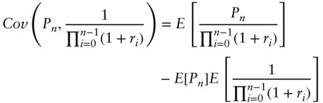
Applying this to two random variables from the previous section, namely, ![]() and
and ![]() ,
,
Let ![]() be the accrued interest on the bond as of date
be the accrued interest on the bond as of date ![]() . Because accrued interest is not a random variable,
. Because accrued interest is not a random variable, ![]() . Next, substitute the definitions of
. Next, substitute the definitions of ![]() ,
, ![]() , and
, and ![]() from Equations (A11.5), (A11.6), and (A11.14) into Equation (A11.16) to see that,
from Equations (A11.5), (A11.6), and (A11.14) into Equation (A11.16) to see that,
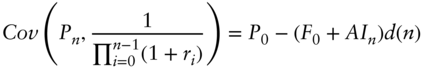
Rearranging terms, substituting in the forward price from Equation (A11.7), and recognizing that ![]() ,
,
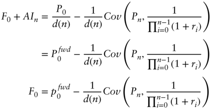
Finally, because bond prices are negatively correlated with interest rates, the covariance term in Equation (A11.18) is negative and, therefore,
The futures price is less than the forward price.
A11.4 FUTURES DELIVERY OPTIONS IN A TERM STRUCTURE MODEL
Having set up a term structure model in the form of a tree, the quality option can be priced as follows. Start at the delivery date. At each node, compute the ratio of the price to conversion factor for each deliverable bond. Find the bond with the minimum ratio and set the futures price equal to that ratio. Then, given these terminal values of the futures price, prices on earlier dates can be computed along the lines described in Section A11.2. In the case of the timing, end‐of‐month, and wild‐card options, which are American‐style options exercisable by the short, the futures price at each node in the tree is the minimum of the futures price with the option exercised and with the option not exercised.
The previous paragraph assumes that the prices of the bonds are available on the tree as of the last delivery date. These bond prices can be computed in one of two ways. If a model with a closed‐form solution for spot rates is being used, then these rates can be used to compute the bond prices as needed. Otherwise, the tree has to be extended to the maturity date of the longest bond in the basket and bond prices have to be computed using the usual tree methodology. The first solution is faster and less subject to numerical error, but a model with a closed‐form solution may or may not be suitable for the problem at hand.
Arbitrage‐free pricing models usually assume that some set of securities is fairly priced. In the case of futures, the standard assumption is that the forward prices of all bonds in the deliverable basket are fair. Technically, this calibration can be accomplished by assigning a spread to each bond such that its forward price in the model matches the forward price in the market. The assumption that bond prices are fair is in the spirit of pricing the futures relative to cash. Another approach can be used to decide whether the underlying bonds are fairly priced or not.
Term structure models commonly used for pricing futures fall into two main categories. First are one‐ or two‐factor short‐rate models along the lines of those described in Chapters 7–9. These models are relatively easy to implement and, for the most part, flexible enough to capture the yield curve dynamics driving futures prices. With only one or two factors, however, these models cannot capture the idiosyncratic price movements of any deliverable bond relative to another.
The second type of model allows for a richer set of relative price movements across bonds in the deliverable basket. These models essentially allow each bond to follow its own price or yield process. There are costs to this flexibility, however. First, ensuring that these models are arbitrage free takes some effort. Second, the user must specify the parameters that describe the stochastic behavior of all bond prices in the basket, for example, a volatility for each of the bonds in the basket along with correlations between each pair of bonds.
Futures traders often describe their models in terms of the beta of each bond in the basket relative to a benchmark bond in the basket. The beta of a bond represents the expected change in yield of that bond given a one‐basis‐point change in the yield of the benchmark. A bond with a beta of 1.02, for example, implies that the bond's yield is assumed to change 2% more than the yield of the benchmark bond. The beta of a particular bond can be thought of as the coefficient from a regression of changes in its yield on changes in the benchmark's yield. Note that in a one‐factor model the beta of a bond is simply the ratio of the volatility of that bond yield to the volatility of the benchmark's yield.