Physical Layer and Data Link Layer
Think of the Physical Layer as the media and signal that support the transmission of signals. A transmission medium can be air (radio frequency), metal (copper unshielded twisted-pair, shielded twisted-pair, or coaxial cable), or glass (optical fiber). Today, the transmission of signals in the fastest but most accurate manner is critical. Digital transmission of 1’s and 0’s must have high speeds with low errors. The Physical Layer is concerned about the transmission of 1’s and 0’s. The Data Link Layer defines the frame format that the 1’s and 0’s are to follow. Frame formats are based on 8 bits or 1 octet, also known as a byte. The frame format is what defines the structure of the 1’s and 0’s being transmitted. Think of the Data Link Layer as the physical envelope that you put the letter in where the letter is composed of a series of 1’s and 0’s.
FIGURE 4-1 depicts the bottom two layers of the OSI model representing the Physical Layer and Data Link Layer, and how they correspond to layers of the related TCP/IP model.
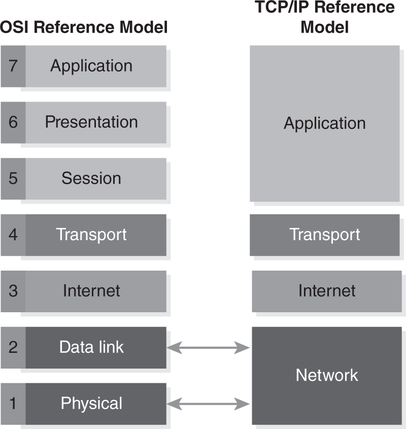
FIGURE 4-1 OSI model compared to TCP/IP model.
Physical Layer: OSI Layer 1
The Physical Layer operates at the bottom layer (Layer 1) of the Open Systems Interconnection (OSI) Reference Model. This layer is where the signaling of 1’s and 0’s occurs. This layer is also where cabling or other transmission media is needed to transmit them. The evolution of communications at the Physical Layer can be traced back to Morse code and the transmission of “dots” and “dashes.” Morse code is named after Samuel F. B. Morse, who invented the telegraph. The telegraph used copper wires to transmit electrical signals to remote stations during the mid-1880s into the early 1990s. These electrical signals translated to letters in the alphabet such that a message could be created and sent.
During the 1960s and 1970s, analog voice communications were used. There were two kinds of telephones in use. The first was the rotary dial telephone. This was followed by dual touch multifrequency (DTMF) telephones. DTMF telephones transmit digits via different voltages.
The voltage signals are sent to the phone company’s central office (CO). This is where phone calls are routed to destination phone numbers. Copper wire was used to send electrical signals or current through the telephony communications network.
Analog and digital communications are most concerned about loss of a signal or loss of the message itself. In other words, this is the loss of a 1 or a 0, or several of them, which can result in a communication error.
 TIP
TIP
Analog communications use alternating current (AC). This is the same type of current that electrical appliances use. AC current continuously changes given it is sent via a sine wave signal. A sine wave has a continuously changing voltage or amplitude signal over time (see FIGURE 4-2).
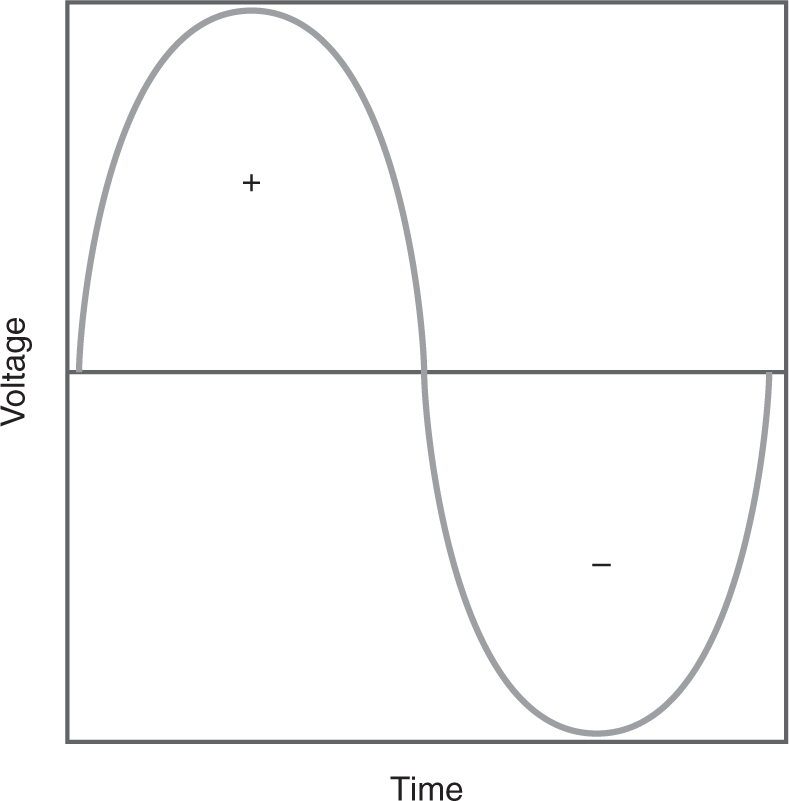
FIGURE 4-2 A sine wave.
Digital communications utilize discrete voltages or values to represent a 1 or a 0 in transmission. Voltage is the indicator for an on (represents a 1) or off (represents a 0) value. This is the same type of direct current (DC) used for battery-powered toys and devices. A square wave is shown in FIGURE 4-3. Notice that it has a discrete on or off value over a specific time.
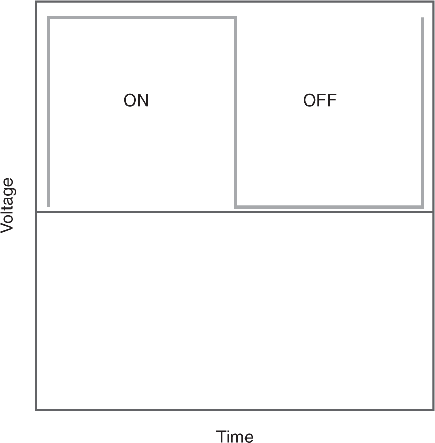
FIGURE 4-3 A square wave.
Depending on the physical media, the bit error rate (BER) will be different. How reliable is the communication link? Which physical media or cable was used? What is the BER of that media? What kind of data is being sent? Is it a data file transfer or real-time multimedia application? Do you need high-speed transmissions with a low BER? This is where the term reliability comes into play. Reliability is the availability and integrity of the data transmission.
These are the design decisions that should be addressed. Availability refers to uptime—whether there is physical link access to the communication line. Integrity refers to whether the data (the 1’s and 0’s) made it to the destination intact and accurate.
The math formula for BER = # of errored bits / total number of bits sent.
 NOTE
NOTE
Communications throughout history utilized the concept of a 1 or 0; examples include smoke signals, Morse code, electrical signals, or sending light. These communication methods can transmit a 1 and 0 or on and off to represent a digital signal and transmission.
Smoke signals were used to notify armies and headquarters at far distances.
Morse code was used with the telegraph system for distant but near-real-time messages.
Electrical signals send rapid streams of 1’s and 0’s to represent complete messages.
Laser or light signals send the fastest streams of 1’s and 0’s to represent complete messages.
TIP
Analog transmissions use sine waves and are measured in frequency. Frequency is the number of cycles per second measured, or hertz. A hertz is one electrical energy cycle from positive voltage (1) to negative voltage (0). Digital transmission uses square waves and is measured as a positive (1) or negative (0) voltage level. If measured in a 1-second time interval, FIGURE 4-4 represents analog versus digital communications.
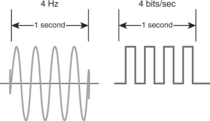
FIGURE 4-4 Hertz versus bits.
Courtesy of Endeavor Business Media, LLC.
Transmission Media
Voltage is what defines a 1 or a 0. To send a lot of them quickly, a cable or transmission medium is needed. We learned that having a low bit error rate is key to supporting high-speed data transmissions such as voice, video, or live gaming. Today, both personal and business communications must support real-time communications. This includes presence/availability, voice, video, instant messaging (IM) chat, conferencing, and collaboration. The more information or data you need to send, the more bits you need to transmit it.
The four most common types of transmission media are:
- Copper—This is used in unshielded twisted-pair (UTP) and shielded twisted-pair (STP) cable. Depending on the application, UTP or STP cabling can be used for low-, medium-, and high-speed transmissions and data networking. UTP is most common in office buildings and wired network environments. UTP is typically used for voice and data communications to the desktop location. TABLE 4-1 lists the various twisted-pair categories and their specifications.
- Coaxial—This is a rugged indoor or outdoor cable. Coaxial cable has an outside insulation protective sheath supported by a metal inner conductor and metallic braided sheath (FIGURE 4-5). The braided sheath surrounds the metal inner conductor. Using radio frequency (RF) coax cable can support greater bandwidth and transmissions at further distances. The cable TV infrastructure is supported by coaxial cable to the residence. The most common types of coaxial cables are:
- RG-6—Typically used for home audio, video, and TV transmission equipment
- RG-58—Typically used for RF transmissions and antennae cabling to radio equipment
- RG-58/U—10Base2 Ethernet, also known as Thinnet
- RG-59/U—Closed circuit television (CCTV) transmission to monitors
- RG-8U—10Base5 Ethernet, also known as Thicknet
- RG-60U—High definition television (HDTV) and high-speed cable modems
- Glass/fiber—Fiber cables have a glass core surrounded by a glass cladding. The glass core is the portion that light travels through. The primary buffer is a protective cover. The outer sheath acts as a jacket to protect the fiber cable. Fiber optics can support large amounts of data transmissions over very far distances. Fiber optics are used for long-haul data transmissions. In addition, fiber optics are used for data centers, campuses, and buildings. Some applications that require high reliability use fiber optic cabling to the desktop. Fiber optic cables typically have multiple strands within the same cable sheath (see FIGURE 4-6). This allows multiple devices to be connected to the ends of each fiber optic strand pair. Single-mode optical equipment and transceivers can operate in bidirectional mode (two directions at one) supporting full-duplex (two-way) communications using a single strand of fiber. A technique called wavelength division multiplexing (WDM) allows multiple wavelengths of light to travel through a single fiber strand, allowing for bidirectional and full-duplex communications.
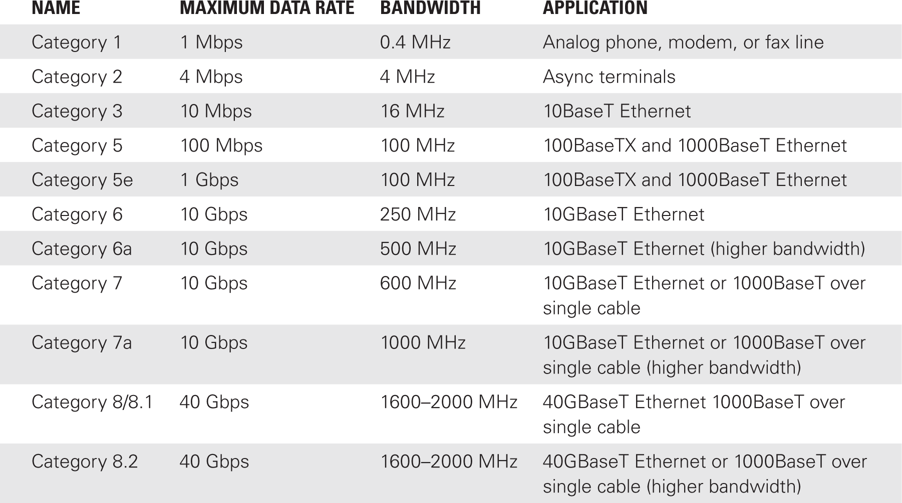
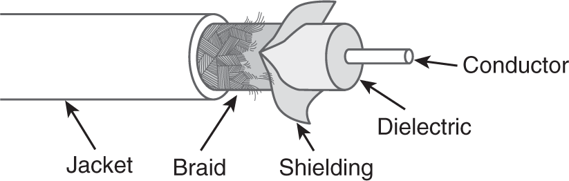
FIGURE 4-5 Anatomy of a coaxial cable.
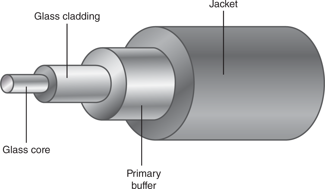
FIGURE 4-6 Anatomy of a fiber optic cable.
Optical devices use transceivers to transmit and receive light signals. Communication equipment uses laser technology to send light through the optical fiber strands (see FIGURE 4-7). Light is measured in wavelengths. Think of a wavelength as the frequency of light or color of light. The optical devices will specify the wavelength of light that the lasers use. This is what your fiber optic cabling must match. There are two kinds of fiber optic cables in use, multimode and single mode.
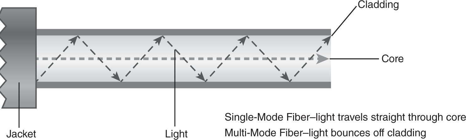
FIGURE 4-7 Today’s multimodal business communication options.
Today’s optical equipment is based on laser technology to send wavelengths of light through a fiber optic cable. High-speed and long-distance fiber cables can support large amounts of bandwidth.
- Air—This is the transmission medium for infrared, satellite, wireless, or radio frequency (RF)–based network technology. How can air impact the transmission of 1’s and 0’s? Air impacts transmission when there is no clear line of sight between two endpoints or the air has moisture such as fog or raindrops. A line of sight between two microwave radio transceivers is shown in FIGURE 4-8. The Fresnel zone is the air space near transceivers that RF signals traverse through.
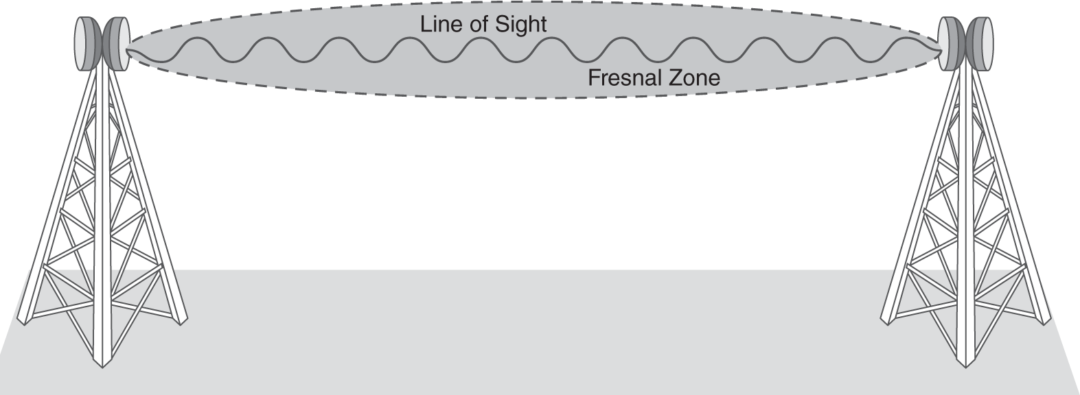
FIGURE 4-8 Line of sight between two microwave radio transceivers.
TIP
The bandwidth you need at your workstation location will define the type of cabling to use. More importantly, installing a cabling system that can support 10+ years of connectivity is desired.
TABLE 4-2 summarizes the bandwidth and BER for the different families of transmission media.
| MEDIA TYPE | BANDWIDTH | PERFORMANCE: TYPICAL ERROR RATE |
|---|---|---|
| UTP—Category 1 (voice grade) UTP—Category 3/4/5/5e/6/6a (high-speed grade) |
1 MHz 10 MHz to 1 GHz |
Poor to fair (10–5) Good (10–7 to 10–9) |
| Coaxial cable | 1 GHz | Good (10–9) |
| Microwave | 100 GHz | Good (10–9) |
| Satellite | 100 GHz | Good (10–9) |
| Fiber | 75 THz | Great (10–11 to 10–13) |
Note that high-speed UTP from Category 3 to Category 6 can support similar bandwidths and BER as coaxial cable but at shorter distances.
Structured Wiring Systems
Businesses need voice and data connectivity to the desktop. New construction projects and building renovations need new wiring. A structured wiring system is a modular cabling solution that is flexible. Structured wiring systems include both outside cabling and indoor cabling. These systems have the following benefits:
- Modular and flexible for supporting end-to-end connectivity
- Support rapid moves, adds, and changes
- Have a lifespan of more than 10 years of operation
- Support high-speed bandwidth and connectivity to the desktop
A structured wiring system has the following parts:
- Workstation outlet and RJ-45 connections—The termination point at the desktop location where twisted-pair cabling is connected to an 8-pin, modular RJ-45 connector
- Intermediate distribution frame (IDF) or wiring closet—The location or room where building backbone cabling terminates to provide connectivity to desktop locations
- Intrabuilding distribution—The cabling that typically emanates from a main distribution frame (MDF) or data center facility to an intermediate distribution frame (IDF) or wiring closets
- Main distribution frame (MDF) or data center—The location or room where backbone cabling terminates to provide connectivity to the data center facility
- Campus or building backbone distribution—The interbuilding cabling that typically consists of fiber optic backbone cabling and twisted-pair bundled cabling to support 10–20 years or more of connectivity for a campus or within a building
FIGURE 4-9 provides a diagram of a structured wiring system in a building.
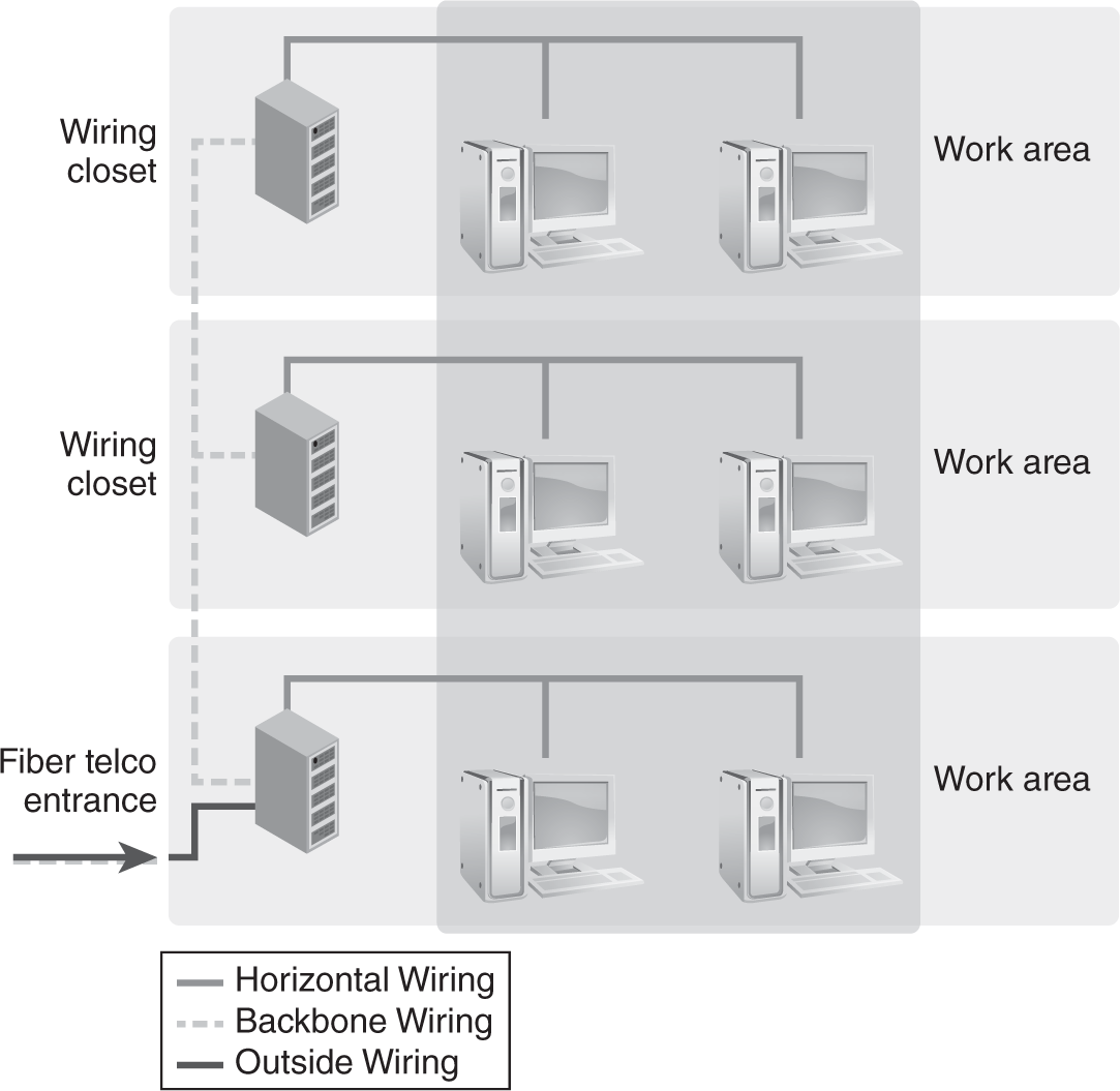
FIGURE 4-9 An example of a structured wiring system.
Technical TIP
RJ-45 connector patch cables are needed to physically connect the workstation to the workstation outlet and the horizontal workstation cabling patch panel to the Ethernet Layer 2 or Layer 3 switch. It is important to verify and confirm the following:
- Workstation outlet RJ-45 connector pin configuration used: TIA-568A or TIA-568B
- Wiring closet RJ-45 connector pin configuration patch panel used: TIA-568A or TIA-568B
The only difference between TIA-568A and TIA-568B is that the orange pair is swapped for the green pair in the RJ-45 connector. For Ethernet LANs that utilize UTP transmission media, the TIA-568B pin configuration is typically used for all RJ-45 connectors and patch panels.
Refer to FIGURE 4-10 for the TIA-568A and TIA-568B pin configurations.
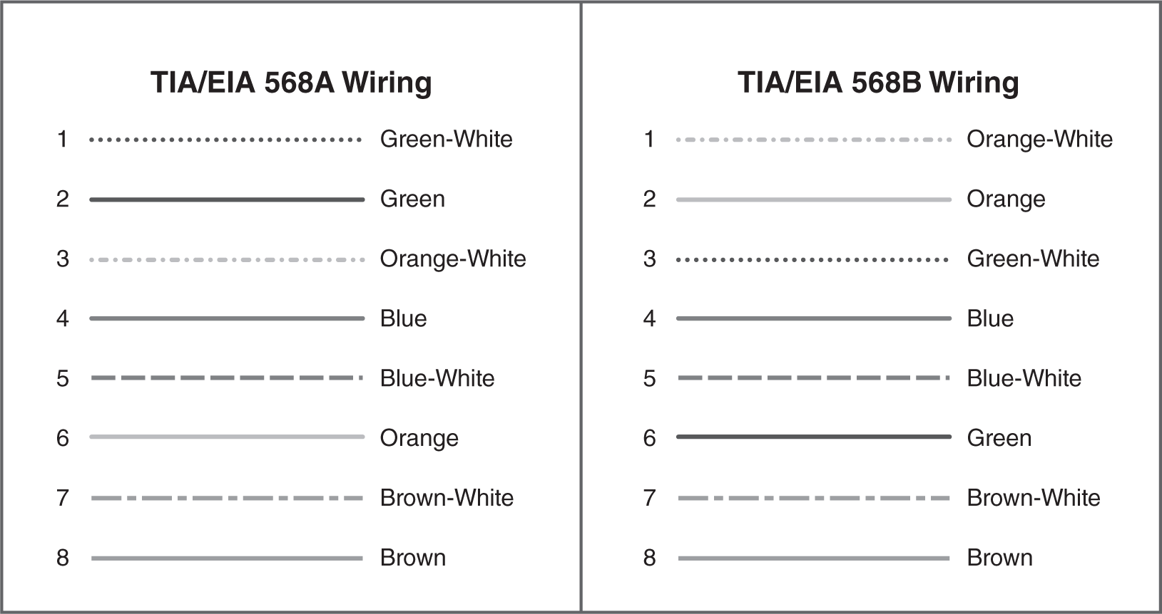
FIGURE 4-10 RJ-45 connector pin configurations.
Once you select which version of the RJ-45 pin-configuration to use, the RJ-45 patch cables you select must also match the pin configuration selected.
A crossover cable has a crossover pin configuration with the orange pair inserted where the green pair would normally be positioned on one end, creating a crossover connection. This is the equivalent of a 568A termination with the other end being 568B terminated. Crossover cables are used to connect two devices directly without the use of a switch. Most switches today can auto-detect if a straight-through or crossover patch cable is used and can enable link integrity regardless.
Straight-through patch cables have each pin and colored wire connected to the exact same pin on the other end of the RJ-45 connector. Both sides are wired as either TIA-568A or TIA-568B.
FIGURE 4-10 provides a diagram of the TIA-568A and TIA-568B pin configurations.
Structured Wiring Standards
Structured wiring systems are supported by both national and international wiring standards. There are several resources available for wiring standards. The three primary sources for wiring standards are:
- Building Industry Consulting Service International (BICSI)—BICSI was created in 1984 when the AT&T monopoly was broken up. This led to on-premise wiring being the responsibility of the building owner, tenant, or homeowner. BICSI has developed standards for cabling distribution systems and the installation of both outdoor and indoor cable plants (http://www.bicsi.org).
- Electronics Industries Association (EIA)—EIA was the original association hired to develop telecommunication wiring standards; it later became the Electronic Components Industries Association (ECIA). The standards were adopted by the Telecommunications Industry Association (TIA), hence the TIA/EIA designation (https://www.ecianow.org).
- Telecommunications Industry Association (TIA)—The current owner of the TIA/EIA 568 standards family, TIA was accredited by the American National Standards Institute (ANSI) to develop and publish industry standards with input from manufacturers and members of the association. TIA is closely linked to telecommunication and communication manufacturers and currently represents approximately 400 companies (http://standards.tiaonline.org/all-standards/committees/tr-42).
NOTE
For additional information, a primer on structured wiring systems is included as an appendix to the textbook.
Data Link Layer: OSI Layer 2
On top of the Physical Layer in the OSI model sits the Data Link Layer. This is where it all comes together on a LAN, from an electrical signaling and frame format perspective. Without the Data Link Layer, computers cannot communicate with servers. The Data Link Layer does exactly that—it prepares the data to be placed onto the physical link.
Data Link Layer Sublayers
There are two sublayers to the Data Link layer that support different functions:
- Media Access Control (MAC)—The MAC sublayer controls access to the media. This is where the Ethernet transceiver operates and interfaces with the Physical Layer. This sublayer listens to the network, and transmits or receives Ethernet frames onto the physical network. This listening is the carrier sense of carrier sense multiple access with collision detection (CSMA/CD). This will be discussed further in the next section.
- Logical Link Control (LLC)—The LLC sublayer controls linking logically. The LLC sublayer sits above the MAC sublayer and acts like a traffic cop, organizing the upper layer protocols into their MAC layer frame prior to transmission onto the network. Think of the LLC sublayer as the flow and error control traffic cop. It allows multipoint communications over a computer network.
FIGURE 4-11 provides a diagram of the Data Link Layer and its sublayers.
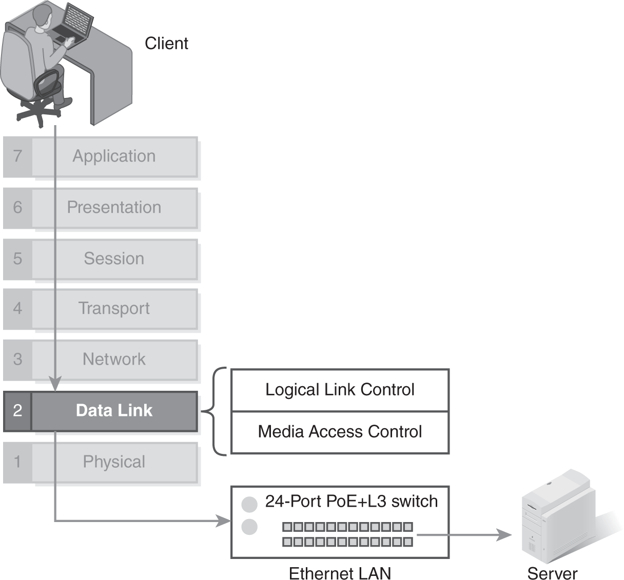
FIGURE 4-11 The Data Link Layer and its sublayers.