

2.3
C
C
loudRenderi
Fi
gu
Soft
w
Fi
gu
(ins
e
ngTechniqu
e
u
re 2.2. Volu
m
w
are, LL
C
.)
u
re 2.3. Wirefr
e
t). (Image cou
r
e
s
m
etric cloud d
a
ame overlay o
r
tesy Sundog
S
a
ta rendered u
s
f splatted clo
u
S
oftware, LL
C
.
s
ing splatting.
u
ds with the si
n
)
(
I
mage court
e
n
gle cloud pu
f
e
sy of Sundog
f
f texture used
31
32 2.Modeling,Lighti ng,andRenderingTechniquesforVolumetricClouds
Lighting and rendering are achieved in separate passes. In each pass, we set
the blending function to (
ONE, ONE_MINUS_SRC_ALPHA) to composite the voxels
together. In the lighting pass, we set the background to white and render the
voxels front to back from the viewpoint of the light source. As each voxel is ren-
dered, the incident light is calculated by multiplying the light color and the frame
buffer color at the voxel’s location prior to rendering it; the color and transparen-
cy of the voxel are then calculated as above, stored, and applied to the billboard.
This technique is described in more detail by Harris [2002].
When rendering, we use the color and transparency values computed in the
lighting pass and render the voxels in back-to-front order from the camera.
To prevent breaking the illusion of a single, cohesive cloud, we need to en-
sure the individual billboards that compose it aren’t perceptible. Adding some
random jitter to the billboard locations and orientations helps, but the biggest is-
sue is making sure all the billboards rotate together in unison as the view angle
changes. The usual trick of axis-aligned billboards falls apart once the view angle
approaches the axis chosen for alignment. Our approach is to use two orthogonal
axes against which our billboards are aligned. As the view angle approaches the
primary axis (pointing up and down), we blend toward using our alternate (or-
thogonal) axis instead.
To ensure good performance, the billboards composing a cloud must be ren-
dered as a vertex array and not as individual objects. Instancing techniques
and/or geometry shaders may be used to render clouds of billboards from a single
stream of vertices.
While splatting is fast for sparser cloud volumes and works on pretty much
any graphics hardware, it suffers from fill rate limitations due to high depth com-
plexity. Our lighting pass also relies on pixel read-back, which generally blocks
the pipeline and requires rendering to an offscreen surface in most modern
graphics APIs. Fortunately, we only need to run the lighting pass when the light-
ing conditions change. Simpler lighting calculations just based on each voxel’s
depth within the cloud from the light direction may suffice for many applications,
and they don’t require pixel read-back at all.
VolumetricSlicing
Instead of representing our volumetric clouds with a collection of 2D billboards,
we can instead use a real 3D texture of the cloud volume itself. Volume render-
ing of 3D textures is the subject of entire books [Engel et al. 2006], but we’ll give
a brief overview here.
The general idea is that some form of simple proxy geometry for our volume
is rendered using 3D texture coordinates relative to the volume data. We then get
2.3CloudRenderingTechniques 33
the benefit of hardware bilinear filtering in three dimensions to produce a smooth
image of the 3D texture that the proxy geometry slices through.
In volumetric slicing, we render a series of camera-facing polygons that di-
vide up the volume at regular sampling intervals from the volume’s farthest point
from the camera to its nearest point, as shown in Figure 2.4. For each polygon,
we compute the 3D texture coordinates of each vertex and let the GPU do the
rest.
It’s generally easiest to do this in view coordinates. The only hard part is
computing the geometry of these slicing polygons; if your volume is represented
by a bounding box, the polygons that slice through it may have anywhere from
three to six sides. For each slice, we must compute the plane-box intersection and
turn it into a triangle strip that we can actually render. We start by transforming
the bounding box into view coordinates, finding the minimum and maximum z
coordinates of the transformed box, and dividing this up into equidistant slices
along the view-space z-axis. The Nyquist-Shannon sampling algorithm [Nyquist
1928] dictates that we must sample the volume at least twice per voxel diameter
to avoid sampling artifacts.
For each sample, we test for intersections between the x-y slicing plane in
view space and each edge of the bounding box, collecting up to six intersection
points. These points are then sorted in counterclockwise order around their center
and tessellated into a triangle strip.
The slices are then rendered back to front and composited using the blending
function (
ONE, ONE_MINUS_SRC_ALPHA). As with splatting, the lighting of each
voxel needs to be done in a separate pass. One technique is to orient the slicing
planes halfway between the camera and the light source, and accumulate the
voxel colors to a pixel buffer during the lighting pass. We then read from this
pixel buffer to obtain the light values during the rendering pass [Ikits et al. 2007].
Figure 2.4. Slicing proxy polygons through a volume’s bounding box.

34
Unfortu
n
quently,
end, we
GPUR
a
Real-ti
m
and mo
s
the com
p
are achi
e
square
k
cond on
The
(with b
a
each fra
g
from th
e
We the
n
to back,
Figure 2
casting. (
I
2.M
o
n
ately, half-
a
and we’re s
t
really haven’
a
yCasting
m
e ray castin
g
t elegant tec
h
p
uting in a fr
a
e
vable with
p
k
ilometer str
a
consume
r
-gr
a
general idea
a
ck-face culli
n
g
ment of the
b
e
camera and
n
sample our
3
compositing
.5. Volumetri
c
I
mage courtes
y
o
deling,Lighti
a
ngle slicing
t
ill left with
m
t gained muc
g
may sound
i
h
nique for re
n
a
gment prog
r
p
recise pe
r
-fr
a
a
tocumulus c
l
a
de hardwar
e
is to just re
n
n
g enabled)
a
b
ounding bo
x
computes th
e
3
D cloud tex
t
the results as
c
cloud data r
e
y
Sundog Soft
w
ng,andRen
d
requires sa
m
m
assive dem
a
h over splatti
i
ntimidating,
b
n
dering clou
d
r
am, but if op
t
a
gment light
i
l
oud layer re
n
e
using GPU
r
der the boun
d
a
nd let the fr
x
, our fragm
e
e
ray’s inters
t
ure along th
e
we go.
e
ndered from
a
w
are, LLC.)
d
eringTechni
m
pling the vo
a
nds on fill r
i
ng.
b
ut in many
w
d
s. It does in
v
t
imized care
f
i
ng. Figure 2
n
dering at o
v
r
ay casting.
d
ing box ge
o
r
agment proc
e
e
nt program s
h
s
ection with t
h
e
ray within t
h
a
single bound
i
quesforVol
u
lume even
m
r
ate as a resu
l
w
ays i
t
’s the
v
olve placin
g
f
ully, high fr
a
.5 shows a
d
v
er 70 frame
s
o
metry of yo
u
e
ssor do the
r
hoots a ray t
h
t
he bounding
h
e volume fr
o
i
ng box using
u
metricClou
d
m
ore fre-
l
t. In the
simplest
g
most of
a
me rates
d
ense, 60
s
per se-
u
r clouds
rest. For
h
rough it
volume.
o
m front
GPU ray
d
s

2.3CloudRenderingTechniques 35
The color of each sample is determined by shooting another ray to it from the
light source and compositing the lighting result using multiple forward scatter-
ing—see Figure 2.6 for an illustration of this technique.
It’s easy to discard this approach, thinking that for every fragment, you need
to sample your 3D texture hundreds of times within the cloud, and then sample
each sample hundreds of more times to compute its lighting. Surely that can’t
scale! But, there’s a dirty little secret about cloud rendering that we can exploit to
keep the actual load on the fragment processor down: clouds aren’t really all that
transparent at all, and by rendering from front to back, we can terminate the pro-
cessing of any given ray shortly after it intersects a cloud.
Recall that we chose a voxel size on the order of 100 meters for multiple
forward scattering-based lighting because in larger voxels, higher orders of scat-
tering dominate. Light starts bouncing around shortly after it enters a cloud, mak-
ing the cloud opaque as soon as light travels a short distance into it. The mean
free path of a cumulus cloud is typically only 10 to 30 meters [Bouthors et al.
2008]—beyond that distance into the cloud, we can safely stop marching our ray
into it. Typically, only one or two samples per fragment really need to be lit,
which is a wonderful thing in terms of depth complexity and fill rate.
The first thing we need to do is compute the intersection of the viewing ray
for the fragment with the cloud’s axis-aligned bounding box. To simplify our
calculations in our fragment program, we work exclusively in 3D texture coordi-
nates relative to the bounding box, where the texture coordinates of the box range
from 0.0 to 1.0. An optimized function for computing the intersection of a ray
with this unit cube is shown in Listing 2.3.
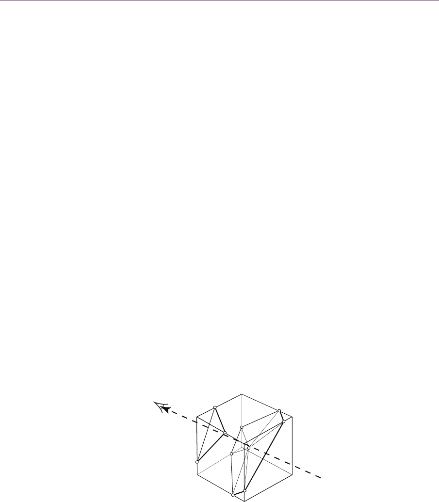
Figure 2.6. GPU ray casting. We shoot a ray into the volume from the eye point, termi-
nating once an opacity threshold is reached. For each sample along the ray, we shoot an-
other ray from the light source to determine the sample’s color and opacity.
..................Content has been hidden....................
You can't read the all page of ebook, please click here login for view all page.