
370 22.GPGPUClothSimulationUsing GLSL,OpenCL,andCUDA
0,1
. A particle is identified by its array index i, which is related to the row and
the column in the grid as follows:
,
mod
i
i
row i n
col i n
.
From the row and the column of a particle, it is easy to access its neighbors by
simply adding an offset to the row and the column, as shown in the examples in
Figure 22.2.
The pseudocode for calculating the dynamics of the particles in an
nn
grid
is shown in Listing 22.1. In steps 1 and 2, the current and previous positions of
the the i-th particle are loaded in the local variables
t
i
p
os
and
1t
i
p
os
, respectively,
and then the current velocity
t
i
vel
is estimated in step 3. In step 4, the total force
i
f
orce
is initialized with the gravity value. Then, the for loop in step 5 iterates
over all the neighbors of
i
p
(steps 5.1 and 5.2), spring forces are computed (steps
5.3 to 5.5), and they are accumulated into the total force (step 5.6). Each neigh-
bor is identified and accessed using a 2D offset
offset offset
,
x
y
from the position of
i
p
within the grid, as shown in Figure 22.2. Finally, the dynamics are computed
in step 6, and the results are written into the output buffers in steps 7 and 8.
for each particle
i
p
1.
t
ii
t
p
os x
2.
1
Δ
t
ii
tt
p
os x
3.
1
Δ
ttt
iii
t
vel
p
os
p
os
4.
i
f
orce
= (0, -9.81, 0, 0)
5. for each neighbor
offset offset
,
ii
row x col y
if
offset offset
,
ii
row x col y
is inside the grid
5.1.
neigh offset offset
*
ii
i
row y n col x
5.2.
neigh neigh
t
t
p
os x
5.3.
rest offset offset
,dxyn
5.4.
curr neigh
tt
i
d
p
os
p
os
5.5.
spring
f
orce
=
neigh
curr rest
neigh
tt
i
t
i
tt
i
ddk b
pos pos
vel
pos pos
5.6.
i
f
orce +=
spring
f
orce
6.
1t
i
p
os =
1
2
tt
ii
pos pos +
2
Δ
i
mt
force
7.
1t
ii
t
xpos
8.
Δ
t
ii
ttxpos
Listing 22.1. Pseudocode to compute the dynamics of a single particle i belonging to the nn
grid.

22.5GPUImplementations 371
22.5GPUImplementations
The different implementations for each GPGPU computing platform (GLSL,
OpenCL, and CUDA) are based on the same principles. We employ the so-called
“ping-pong” technique that is particularly useful when the input of a simulation
step is the outcome of the previous one, which is the case in most physically-
based animations. The basic idea is rather simple. In the initialization phase, two
buffers are loaded on the GPU, one buffer to store the input of the computation
and the other to store the output. When the computation ends and the output
buffer is filled with the results, the pointers to the two buffers are swapped such
that in the following step, the previous output is considered as the current input.
The results data is also stored in a vertex buffer object (VBO), which is then used
to draw the current state of the cloth. In this way, the data never leaves the GPU,
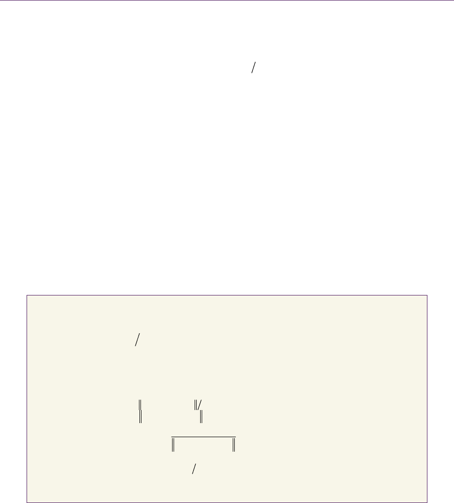
achieving maximal performance. This mechanism is illustrated in Figure 22.4.
Figure 22.4. The ping-pong technique on the GPU. The output of a simulation step be-
comes the input of the following step. The current output buffer is mapped to a VBO for
fast visualization.
Buffer 0
tx
Δttx
GPU
computation
Buffer 1
Vertex
Buffer
Object
GPU
Input Output
1. Odd simulation steps (ping...)
Buffer 1
tx
Δttx
GPU
computation
Buffer 0
Vertex
Buffer
Object
GPU
Output Input
2. Even simulation steps (...pong)
Draw
Draw
372 22.GPGPUClothSimulationUsing GLSL,OpenCL,andCUDA
22.6GLSLImplementation
This section describes the implementation of the algorithm in GLSL 1.2. The
source code for the vertex and fragment shaders is provided in the files
ver-
let_cloth.vs
and verlet_cloth.fs, respectively, on the website. The position
and velocity arrays are each stored in a different texture having
nn
dimensions.
In such textures, each particle corresponds to a single texel. The textures are up-
loaded to the GPU, and then the computation is carried out in the fragment
shader, where each particle is handled in a separate thread. The updated state
(i.e., positions, previous positions, and normal vectors) is written to three distinct
render targets.
Frame buffer objects (FBOs) are employed for efficiently storing and access-
ing the input textures and the output render targets. The ping-pong technique is
applied through the use of two frame buffer objects, FBO1 and FBO2. Each FBO
contains three textures storing the state of the particles. These three textures are
attached to their corresponding FBOs as color buffers using the following code,
where
fb is the index of the FBO and texid[0], texid[1], and texid[2] are
the indices of the textures storing the current positions, the previous positions,
and the normal vectors of the particles, respectively:
glBindFramebufferEXT(GL_FRAMEBUFFER_EXT, fbo->fb);
glFramebufferTexture2DEXT(GL_FRAMEBUFFER_EXT,
GL_COLOR_ATTACHMENT0_EXT, GL_TEXTURE_2D, texid[0], 0);
glFramebufferTexture2DEXT(GL_FRAMEBUFFER_EXT,
GL_COLOR_ATTACHMENT1_EXT, GL_TEXTURE_2D, texid[1], 0);
glFramebufferTexture2DEXT(GL_FRAMEBUFFER_EXT,
GL_COLOR_ATTACHMENT2_EXT, GL_TEXTURE_2D, texid[2], 0);
In the initialization phase, both of the FBOs holding the initial state of the
particles are uploaded to video memory. When the algorithm is run, one of the
FBOs is used as input and the other one as output. The fragment shader reads
the data from the input FBO and writes the results in the render targets of the
output FBO (stored in the color buffers). We declare the output render targets by
using the following code, where
fb_out is the FBO that stores the output:
glBindFramebufferEXT(GL_FRAMEBUFFER_EXT, fb_out);
GLenum mrt[] = {GL_COLOR_ATTACHMENT0_EXT,
GL_COLOR_ATTACHMENT1_EXT, GL_COLOR_ATTACHMENT2_EXT};
glDrawBuffers(3, mrt);
22.7CUDAImplementation 373
In the next simulation step, the pointers to the input and output FBOs are
swapped so that the algorithm uses the output of the previous iteration as the cur-
rent input.
The two FBOs are stored in the video memory, so there is no need to upload
data from the CPU to the GPU during the simulation. This drastically reduces the
amount of data bandwidth required on the PCI-express bus, improving the per-
formance. At the end of each simulation step, however, position and normal data
is read out to a pixel buffer object that is then used as a VBO for drawing pur-
poses. The position data is stored into the VBO directly on the GPU using the
following code:
glReadBuffer(GL_COLOR_ATTACHMENT0_EXT);
glBindBuffer(GL_PIXEL_PACK_BUFFER, vbo[POSITION_OBJECT]);
glReadPixels(0, 0, texture_size, texture_size,
GL_RGBA, GL_FLOAT, 0);
First, the color buffer of the FBO where the output positions are stored is select-
ed. Then, the positions’ VBO is selected, specifying that it will be used as a pixel
buffer object. Finally, the VBO is filled with the updated data directly on the
GPU. Similar steps are taken to read the normals’ data buffer.
22.7CUDAImplementation
The CUDA implementation works similarly to the GLSL implementation, and
the source code is provided in the files
verlet_cloth.cu and ver-
let_cloth_kernel.cu
on the website. Instead of using FBOs, this time we use
memory buffers. Two pairs of buffers in video memory are uploaded into video
memory, one pair for current positions and one pair for previous positions. Each
pair comprises an input buffer and an output buffer. The kernel reads the input
buffers, performs the computation, and writes the results in the proper output
buffers. The same data is also stored in a pair of VBOs (one for the positions and
one for the normals), which are then visualized. In the beginning of the next it-
eration, the output buffers are copied in the input buffers through the
cudaMemcpyDeviceToDevice call. For example, in the case of positions, we
use the following code:
cudaMemcpy(pPosOut, pPosIn, mem_size, cudaMemcpyDeviceToDevice);
It is important to note that this instruction does not cause a buffer upload from
the CPU to the GPU because the buffer is already stored in video memory. The
374 22.GPGPUClothSimulationUsing GLSL,OpenCL,andCUDA
output data is shared with the VBOs by using graphicsCudaResource objects,
as follows:
// Initialization, done only once.
cudaGraphicsGLRegisterBuffer(&cuda_vbo_resource, gl_vbo,
cudaGraphicsMapFlagsWriteDiscard);
// During the algorithm execution.
cudaGraphicsMapResources(1, cuda_vbo_resource, 0);
cudaGraphicsResourceGetMappedPointer((void **) &pos,
&num_bytes, cuda_vbo_resource);
executeCudaKernel(pos, ...);
cudaGraphicsUnmapResources(1, cuda_vbo_resource, 0);
In the initialization phase, we declare that we are sharing data in video memory
with OpenGL VBOs through CUDA graphical resources. Then, during the exe-
cution of the algorithm kernel, we map the graphical resources to buffer pointers.
The kernel computes the results and writes them in the buffer. At this point, the
graphical resources are unmapped, allowing the VBOs to be used for drawing.
22.8OpenCLImplementation
The OpenCL implementation is very similar to the GLSL and CUDA implemen-
tations, except that the data is uploaded at the beginning of each iteration of the
algorithm. At the time of this writing, OpenCL has a rather young implementa-
tion that sometimes leads to poor debugging capabilities and sporadic instabili-
ties. For example, suppose a kernel in OpenCL is declared as follows:
__kernel void hello(__global int *g_idata);
Now suppose we pass input data of some different type (e.g., a float) in the fol-
lowing way:
float input = 3.0F;
cfloatlSetKernelArg(ckKernel, 0, sizeof(float), (void *) &input);
clEnqueueNDRangeKernel(cqQueue, ckKernel, 1, NULL,
&_szGlobalWorkSize, &_szLocalWorkSize, 0, 0, 0);
When executed, the program will fail silently without giving any error message
because it expects an
int instead of a float. This made the OpenCL implemen-
tation rather complicated to develop.
..................Content has been hidden....................
You can't read the all page of ebook, please click here login for view all page.