
Chapter 15
Standard Projection Techniques
Introduction to Standard Projections
When working with images for texturing, we have to define exactly how the image is to be placed (projected) onto the surface of the object, as no program is so intelligent as to know exactly how to place an image onto a surface without some coordinates that tell it where to put the image and in what manner the image should be applied. Even in the adjacent image, we would need to tell LightWave how to project this texture straight onto the surface, even though the placement may seem pretty straightforward and obvious.
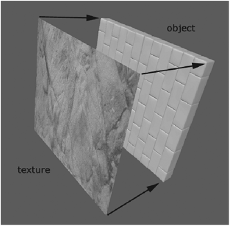
Figure 15-1
Defining these projections involves a process called mapping, of which there are a number of different types. Mapping can be roughly divided into two main categories: standard projections and UV mapping. Both offer a few different options for you to use, and are suitable for different situations.
To use a real-life analogy, let’s assume that you make a sculpture and then paint all the surface detail for that sculpture onto a piece of cloth. Okay, I know it would be a bit odd to not just paint directly onto the surface, but bear with me here! So you have your sculpture, and you have your cloth, and now you need to figure out a way of wrapping the cloth onto the sculpture so that it looks right. That is basically what mapping is. Do you stick the cloth straight onto the front of the sculpture or do you strategically arrange the cloth onto it?
NOTE: You only have to specify a projection type for images and for a few procedural textures, as gradients and most procedurals do not require them due to the way that they are created.
What makes mapping really challenging is that in any situation, a number of different approaches could be applicable. The trick is to choose the best one, and deciding on that requires a bit of planning and thought.
To define the manner in which an image will be projected onto a surface, you need to choose an option from the Projection list in the Texture Editor for the channel into which you are placing the image.
As you can see, there are quite a few choices.

Figure 15-2
The first five options in the list — Planar, Cylindrical, Spherical, Cubic, and Front — are standard (basic) projection types. Standard projection types offer perhaps the most straightforward methods of placing textures onto your surface. All you have to do is decide on the most appropriate method for the object upon which you need to apply the texture, as the choice you make will really depend on the shape and orientation of the surface with which you are working.
Planar Projection
Using Planar Projections
Planar is probably the simplest method to use of all the standard projection types. It is also possibly the most popular way of placing textures onto surfaces. Its simplicity can be deceiving though, because as straightforward as it is, this option is by no means simplistic or stunted in its actual use. In fact, you could almost say that as a general rule of thumb, if an object cannot be planar mapped, then it cannot be mapped. Sure, for some objects, planar mapping the entire thing would be quite a task, but nevertheless it is totally possible.
Anyway, enough waffling about all that, as you are probably wanting to know exactly what this simple method is!
Planar projection basically takes an image and projects it straight along an axis, through the surface.
Applying an Image Using Planar Projection
We apply an image by selecting Planar from the Projection list in the Texture Editor, and then deciding which axis to project the image along by clicking on it in the Texture Axis option.
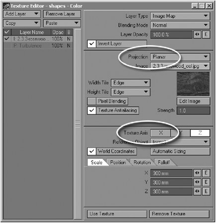
Figure 15-3
This is demonstrated in Figure 15-4. As you can see, we take an image and simply slap it straight onto the object along the same axis that the front of the object is facing.

Figure 15-4
So basically all you do is consider the direction in which the surface is oriented, and then apply the image along that axis. In this case, the surface of the object is facing sideways, so we basically apply the planar image along the x-axis.
Likewise, if the surface faces upward or downward, we would apply it along the y-axis, whereas if it were facing toward the front or back, we would project along the z-axis.
Planar Stretching/Dragging
Now if we look closely at the object with the texture applied, we notice a slight problem. Do you see how the texture stretches through the length of the object, leaving those rather unsightly lines? This is an unfortunate problem that we always face when using planar projections.

Figure 15-5
Think of it like this. Say we have a block, and we have a nice little piece of paper with a little design on it that is the size of one of the block’s sides. To apply that paper design onto the block, we would simply take the piece of paper and stick it onto one side of the block.
However, because the piece of paper is flat and only the size of one side, we cannot bend it around the edges of the block, so instead it just stays stuck on the side that we have glued it onto. Similarly, a planar projection cannot bend around edges; it simply stays stuck on the face that you have applied it to, along the parts of the face that are oriented in the same direction as the axis that you have projected it along. Planar mapping obviously works like a plane (hence the name), and as you probably know from modeling, you cannot bend planes, because in reality that is impossible.

Figure 15-6
So how does this explain the nasty stretching shown in Figure 15-7? Well, consider this. If the design on this piece of paper that you have stuck on your block has been painted onto the paper, and the paint is still wet, you could try to get the design that is painted onto it onto the other sides of the box by smearing the wet paint along the edges of the paper along the surrounding sides of the box. This would look pretty hideous.
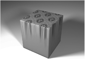
Figure 15-7
Think of the pixels at the edge of an image being like the wet edges of that piece of paper. Now does that make sense? Obviously the best way to get the design onto each side of the box would be to stick a piece of paper with the design on it onto each side of the block, not by smearing the paint.
In LightWave, you could do this by using a combination of a couple of different planar projections along different axes, so that the image could be projected onto each side correctly. The easiest way to do this would be to assign different surfaces to the block according to their orientation and then simply project the images accordingly, as in Figure 15-8.

Figure 15-8
In this example, I have assigned three different surfaces to the box, one for each projection axis. So basically the top and bottom polygons have one surface assigned to them with the image projected along the y-axis, the side polygons have one surface applied to them with the image projected along the x-axis, and the front and back polygons share a surface with the image projected along the z-axis.
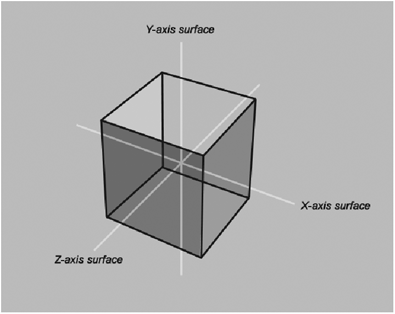
Figure 15-9
This, however, is not the only method. Instead of assigning separate surfaces, you could also apply a single surface to the entire box and simply set up three different layers within the Texture Editor, each with its appropriate planar projection. You could then use falloff (covered in Chapter 13) to ensure that none of that nasty planar stretching is visible.
So now we understand how planar mapping works on objects like blocks, but what about uneven surfaces? Well, you can use planar mapping on some irregular surfaces, but surfaces that are very uneven cause problems, because that horrible stretching that happened in the block example becomes visible. In Figure 15-10, I have projected the dirt texture along the y-axis, and as you can see, this works fine with the fairly flat surface, but when applied to the very irregular surface, we get stretching.

Figure 15-10
Although you could probably get away with this sort of thing in a distance shot, it will not suffice for objects that are close to the camera.
As you can see, the more the surface slopes away along the projection axis, the worse this problem becomes, as more stretching appears.

Figure 15-11
This makes planar mapping really mostly ideal for flattish objects such as walls, doors, floors, or any polygonal surface that is predominantly facing toward one axis and does not have too much visible depth where stretching would occur.
Blending Planar Projections
As I mentioned at the beginning of this chapter, pretty much any object of any type or structure can technically be planar mapped. Sometimes, however, this requires you to use a number of different images projected along different axes that you blend together using falloff in each texture layer that needs a different projection axis, or by using gradients (especially with weight maps) as alpha layers, or even alpha channels in the images themselves. Sounds complex, but it is actually fairly logical and simple to execute.
Blending with Falloff
The most logical way of blending planar projections would be by using falloff on each layer that needs to be blended, and then carefully positioning each image so that it all works nicely.
NOTE: For more detailed information on using the Falloff options in the Texture Editor, please refer to Chapter 13.
Using the same irregular ground object from the previous example, all I have to do is create two separate layers in the Texture Editor, each with the dirt image in it. One of the layers is projected along the y-axis, as before, while the other is projected along the z-axis. The image that is projected along the y-axis will not have to have any falloff settings applied to it, because in this instance, it will be on the bottom layer, while the other layer will blend with it from above.
But let’s do this step by step so that everything is very clear.
So, starting right at the beginning, I create one layer in the Texture Editor. Figure 15-12 shows the surface once again, with the image applied along the y-axis only.

Figure 15-12: Texture applied to y-axis
Take a look at where the stretching occurs, and remember that this stretching is happening along the surfaces that slope downward, along the same axis the image is projected along, which is the y-axis. In order to cover up these areas, we need to apply something along the z-axis so that these areas will no longer be visible.
Now let’s add a second layer to the Texture Editor above the bottom layer, this time with the same image projected along the z-axis. This step of the process looks like Figure 15-13.

Figure 15-13: Texture applied to z-axis
Yes, I know this looks wrong, but don’t worry! Once blended correctly, this image will cover up the stretching along the z-axis.
So how do we get these two layers to blend together correctly? Well, all I need to do is add some falloff to the top layer (the one that is projected along the z-axis) and reposition it slightly.
So what I do is set up some falloff to the layer as shown in Figure 15-14.
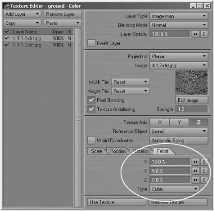
Figure 15-14
The percent of falloff refers to percent per meter of falloff, which means that 100% falloff creates a linear falloff to 0% at 1 meter.
The falloff on the y-axis prevents it from stretching along the bottom of the object, while the falloff on the x-axis prevents the stretching from appearing too much along the sides.
I also shift the actual position of the image slightly upward (to make absolutely sure that the image does not drag along the bottom of the object), and remove all tiling options so that the image does not repeat itself at all by selecting the Reset option in my tiling options (see Chapter 13 for more information on tiling images).
For the sake of this example, I have hidden the bottom layer so that you can see the way in which the falloff and repositioning of this image has faded the image out along the y-axis.
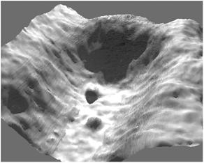
Figure 15-15
As you can see, we have a nice fading that will blend well with the bottom image. Notice that I did not fade it out completely along the side and bottom, as this would basically make the entire image disappear.
When I switch the bottom layer back on and render it, the stretching is covered up by the top layer.
Pretty nifty.
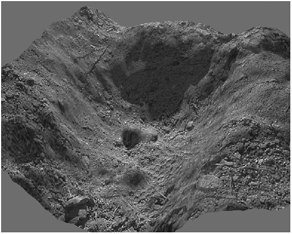
Figure 15-16
Blending with Gradients
The next blending method we can try out is using gradients in conjunction with weight maps. This method is not always as effective as the falloff method, depending on the model, but is nevertheless worth a mention. Although it requires a little more work, it is, in many ways, easier than the falloff method, which can sometimes be a little confusing.
For this method you simply create weight maps that will act as alphas to place the images where you want them to be, and then create gradient layers over those image layers in the Texture Editor, with the appropriate weight map set up as the alpha for that particular image. Let’s examine this process.
Figure 15-17 shows the object and the three images that we wish to apply to the object. For the sake of simplicity I am using a very simple object, a cube, but this principle could be applied to any type of shape. Image 1 will be projected along the x-axis, Image 2 will be projected along the z-axis, and Image 3 will be projected along the y-axis.
First, I need to create a weight map for the object to determine where the different images will be visible. Now remember, once we create the weight map and use it with the gradient, it will act as an alpha layer for the image that we wish to place onto the model. This means that we must create the weight map with a nice solid area of one particular value to determine the area where the image will be visible. So, I start off by creating a new weight map and calling it “texture image 1,” and selecting the areas where I want the image to be visible. I then assign a single value, 100%, to this selection.

Figure 15-17
This area, which has now been assigned a value of 100% in this weight map, can now be used as an alpha layer with Image 1, and the image will only show through this particular part of the weight map.
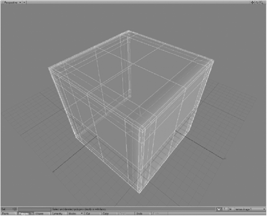
Figure 15-18
I now create a second weight map called “texture image 2” that will act as the alpha for the second image. I do exactly the same thing as for the first one, except that for Image 2 I set the weight map’s value to 100% on the areas that lie along the y-axis.
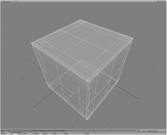
Figure 15-19
And once again, I create yet another weight map, “texture image 3,” that has the 100% area located on the areas of the object that lie along the z-axis.
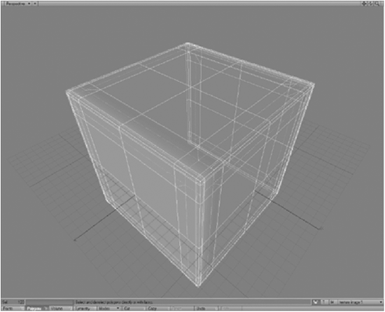
Figure 15-20
I now have three weight maps, each of which will act as an alpha layer for its respective image when applied to the model. I now switch to Layout and begin to set up my surface.
I first apply Image 1 to the color channel of the cube. I set the projection to Planar along the x-axis.
As you can see, the projection is working as per normal planar manner. However, since we only want the image to show up on the parts of the cube that lie along the x-axis, I now create a gradient layer above the image to act as an alpha for it. I set the gradient’s Input Parameter to Weight Map, and select the “texture image 1” weight map. I then create a key in the gradient at 100%, and set the color of that key to white. I also create keys at 0% and 99%, and set the colors of those keys to black. I set the gradient’s Blending Mode to Alpha.

Figure 15-21
This will now allow the image to only show through the areas of the weight map that are 100%, as we can see when the cube is rendered again. See Figure 15-23.

Figure 15-22
I now repeat these steps for the other two images, creating for each of them a gradient that acts as an alpha layer with its corresponding weight map.
Once all of that is done, I have a cube with all three images placed on their correct sides, as shown in Figure 15-24.

Figure 15-23
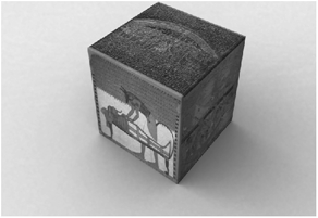
Figure 15-24
So, as you can see, this is actually a very easy way of placing images and controlling them, even though it requires a bit of extra work.
Blending with Alpha Channels
While the weight map and gradient method provides a nice hands-on and visual solution to creating alpha channels within Modeler for your textures, you can, of course, also just create alpha channels within the images themselves. Certain file formats, such as TGA, can support 32-bit image depth that includes an alpha channel embedded in the image itself.
To do this, all you really need to do is to create a falloff along the edges of the image within the alpha channel, as shown in Figure 15-25.
As you can see, this alpha channel in the image would show only the areas that are within the white part of the alpha, so the edges of the image would be invisible when applied to the object.
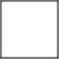
Figure 15-25
If we were to take three images and create an alpha channel like this for each one, and could stack them on top of each other in the Texture Editor on the surface of the cube from the previous example, they would automatically blend together without a problem. Figure 15-26 shows three different images, each applied to a separate axis and blended by using their own alpha channels.

Figure 15-26
The only tricky thing about using this method on an object like this is that the images fade out along the edges of the cube, showing the surface’s color beneath it. So just be sure to make the surface’s color similar to the overall colors of the images.
Cylindrical Projection
Using Cylindrical Projections
Well, you will be happy to know that cylindrical projections are really straightforward. You use them for mapping cylindrical objects — it really is as simple as that. Unlike planar projections that can be used for so many different occasions and in so many ways, cylindrical projections are there for when you are texturing tubes, poles, spears, arms, legs, soda cans, and anything else that is, well, cylindrical in shape.
Applying an Image with Cylindrical Projection
To use a cylindrical projection for a texture, select the Cylindrical option from the Projection list in the Texture Editor.

Figure 15-27
Once you have selected this type, you need to choose an appropriate projection axis from the Texture Axis options. Just like with the planar projections we looked at in the previous section, the axis that you choose for the texture to project along depends on the orientation of the object to which you are applying the texture. Upright cylinders would have the texture applied along the y-axis, whereas cylinders that are lying on their sides would have the texture projected along the x-axis or z-axis, depending on whether they are facing from side to side or front to back respectively.
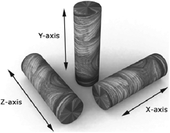
Figure 15-28
Think of it as taking a piece of paper and wrapping it around a tube, because that is essentially what cylindrical mapping does, as demonstrated in Figure 15-29.
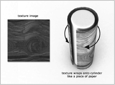
Figure 15-29
“Capping” Cylindrical Objects
As you see, the actual use of this projection type is extremely logical. The only problem that we really face with it, even when using it correctly, is the pinching that happens at either end of the cylinder, on the cylinder “caps.” This really cannot be avoided if the ends of the cylinder have the same surface applied.
Of course, we can use a variety of methods to cover it up, such as using falloff or any of the other methods discussed in the previous section, or we could simply assign a separate surface to the end faces.
Figure 15-30 shows a method using weight maps in combination with gradients to control the visibility of the image on the top. This is using a single surface with the gradient (together with the weight map) being used as an alpha layer on top of the image projected in a planar fashion along the y-axis onto the top part.

Figure 15-30
As you can see, it works quite nicely, and it was really easy to set up. All I did was create a new weight map on the cylinder that had an initial value of 0%, and then selected all the points along the top and bottom of the cylinder and set them to 100%, as shown in Figure 15-31.

Figure 15-31
I then use this weight map, together with a gradient, and set up the gradient so that the image projected onto this section will only show in the areas where the weight map has a value of 100% when the gradient layer is placed above the image layer. We obviously need to use this weight map to avoid the planar stretching that we looked at in the previous section, which would occur from the image on top being projected down the length of the cylinder.
Ensuring Seamless Mapping
It is important when working with cylindrical projections to bear in mind that somewhere along the object the ends of the texture are going to meet. Because of this, you might want to ensure that the image can tile correctly if you do not want any visible seam. Tiling images is placing repeating versions of an image on a surface. Ideally, in order to create a smooth look to the surface, we would not want to be able to see where each copy of the image ends within the pattern, because this would look rather odd. These visible edges are called seams and are generally to be avoided at all costs.
Obviously you are not always working with images that have to have all the seams hidden, as some surfaces, like a soda can, might actually have a visible seam on the label. However, when working with other types of surfaces, especially organic surfaces, you have to make sure that the images are going to meet without any noticeable seams.
Figure 15-32 demonstrates what happens when an image’s two sides do not match, resulting in a seam, and also shows a correctly made image that tiles the right way.

Figure 15-32
As you can see in the example on the left, the image used as a texture has sides that do not match up, resulting in an image that will not be seamless when applied to an object. Notice in the little block below the image itself that when the image is placed alongside itself, you can see the separations at the edge.
In the example on the right, no seams are visible when using this image, as this particular texture is tileable because the edges are matched.
Using Adobe Photoshop’s Offset Filter to Hide Seams
The easiest way to make sure that an image can be tiled is by using the Off-set filter in Adobe Photoshop. If you create an image that you wish to tile on a surface, all you have to do is offset it along the top and one of the sides, and then simply cover up the visible overlapping areas using airbrushing or the cloning tool. Let’s take a look at Figure 15-33, which shows the image used in the previous example that had unmatched sides.
Now, we go to the Offset filter in Photoshop (Filter>Other>Offset), and offset it from the top and the right, both by 100 pixels. We get the result shown in Figure 15-34.
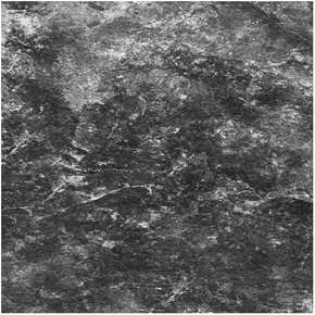
Figure 15-33

Figure 15-34
As you can see, we now have a visible seam within the image itself. All we have to do now is hide it. In this example, I just use the Rubber Stamp (clone) tool. See Figure 15-35.
If we try tiling this image now, we will have no visible seams, as shown in Figure 15-36.

Figure 15-35
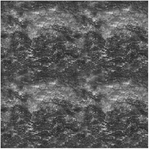
Figure 15-36
And if we were to wrap this around a cylinder, we would have no visible seam either. So that is a nice quick method of ensuring seamless textures!
NOTE: Refer back to Chapter 11 for more information on creating and using seamless textures.
Using the Width Wrap Amount Option
The most astute of you may have noticed that there is an option when using cylindrical projections in the Texture Editor called Width Wrap Amount.

Figure 15-37
The value you enter into this field determines the number of times the texture is wrapped around the object to which it is applied. So if, for example, you wanted to wrap an image around a cylinder five times, you would enter a value of 5 in this field.
Figure 15-38 shows the result of wrapping a texture a total of eight times around the cylinder.
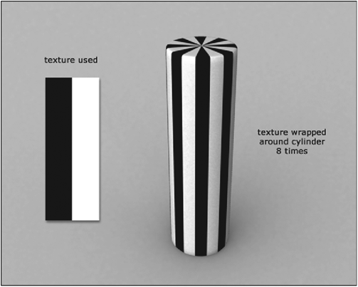
Figure 15-38
Obviously, this is great for adding any repeating details without having to actually make one big image that includes the repeating, especially since smaller images use less memory. In a case like this, it is beneficial to use the simplest, smallest image that you can get away with. Of course this is also a quicker method than creating a long image with the stripes repeated eight times.
Setting your width wrap correctly is also important for preventing an ill-sized image from becoming hideously stretched if it wrapped 360° around an object that the image is technically too small for. Increasing this amount would therefore reduce this stretching by repeating the image more times along those 360°, thereby making each repeat of the image cover less space, and therefore distort less.
Cylindrical Projection Tutorial: Applying a Label to a Soda Can
This tutorial briefly demonstrates the process of applying a label to a can of soda.
1. Open Modeler and load the 4.1.3-sodacan.lwo object from the companion CD. Notice that the can has two separate surfaces applied to it: one surface for the label and one surface for the metal parts.
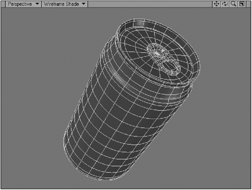
Figure 15-39
2. Open the Surface Editor (Ctrl+F3), and go to the label texture. Click on the “T” button next to the Color channel to open up the Texture Editor.

Figure 15-40
3. Go to the layer list and click where it says “(none).” By default, all new layers created when the Texture Editor is first opened are image layers, so you do not have to specify that this is an image layer. Notice that the default projection type is always Planar. Click on the Projection drop-down button and select Cylindrical. Leave the Width Wrap Amount option that appears at 1.0.

Figure 15-41
4. Click on the Image drop-down button and select Load Image. Find the 4.1.3-sodalabel.jpg image on the companion CD and load it.
As you can see, the image looks a little strange on the can, but we will fix that in a moment.

Figure 15-42
5. Go to where it says Texture Axis and select Y by clicking on that button. This now projects the image down the length of the object (its y-axis) in a cylindrical fashion.

Figure 15-43
6. Now just click on the Automatic Sizing button, and hey, presto! The image fits perfectly onto the soda can as it should. That looks much better.

Figure 15-44
You now have a cool-looking soda can that you can do with as you wish.
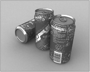
Figure 15-45
Spherical Projection
Using Spherical Projections
As its name suggests, this mapping projection type is for objects that are more or less spherically shaped, or even perfect spheres (of course!). So when it comes to mapping planets, balls, and sometimes also certain kinds of heads, this is the projection to use.
The way it basically works is almost identical to the way that cylindrical mapping works, except that it wraps from both poles (the top and bottom points of the model), creating a single seam along the axis of the model. This means that the image you are using will meet up not only along the seam but also at both poles.
The one thing that sometimes makes this projection type a little tricky to work with is the way in which textures applied shrink toward the poles on the objects. Naturally, you can always work around this to compensate for it, but it can be a little annoying at times.
Figure 15-46 demonstrates this shrinking that occurs toward the poles of the object.

Figure 15-46
You compensate for this effect by altering the image, stretching the top and bottom parts of the texture to compensate for their shrinkage once applied. Of course this sort of alteration might not always be entirely necessary, as you may find that when working with textures for things like planets, this shrinking may not actually be all that noticeable, as shown in Figure 15-47, which uses a totally unaltered rectangular map of the world as a texture.

Figure 15-47
Applying an Image with Spherical Projection
To wrap an image spherically around an object, simply select the Spherical option from the Projection list in the Texture Editor.
You then select an appropriate axis along which you wish to project the image. Most spherical mapping situations use the y-axis.

Figure 15-48

Figure 15-49
You’ll notice that we also have options called Width Wrap Amount and Height Wrap Amount when using spherical projections. Like the Width Wrap Amount for cylindrical projections, here this value simply determines the number of times that the image is repeated as it is wrapped around the width of the model. The Height Wrap Amount value determines the number of times that the image is repeated along the length of the object (as opposed to its breadth). These values basically work as tiling options for this type of projection.
If we change each of these values to 4.0 using our world image, the way in which these values work is clearly illustrated. In Figure 15-50 you can see that the image is repeated four times around the width and four times along the height of the sphere. For most situations, you’ll find that the value of 1.0 is most appropriate.

Figure 15-50
Ensuring Seamless Mapping
As with the cylindrical projections that we looked at in the previous section, spherical projections also have the risk of visible seams on the axis along which we have projected the image.
This means that generally we should always try to ensure that the edges of the image will meet seamlessly.
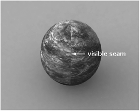
Figure 15-51
Refer back to the previous section on cylindrical mapping and review the technique of using Adobe Photoshop’s Offset filter for correcting this.
However, when dealing with spherical mapping, not only do we have to watch for seams along one side of the object, we also have to be aware of how the image looks when it meets up at the poles.
Using Adobe Photoshop’s Polar Coordinates Filter to Check Seams
A quick and easy way of checking to see how the image will look when applied spherically is to use Photoshop’s Polar Coordinates filter.
This filter is found under the Distort filters in Photoshop. Use it only to check your image, as leaving the filter applied to the image will mess up the image, making it no longer useful for our purposes.
Basically what you do is open the filter’s panel and ensure that the Rectangular to Polar option is selected. The little preview window will show you a decent representation of how the image will more or less behave when wrapped spherically around your model in LightWave.

Figure 15-52
You can use this to ensure that the image is seamless at the poles. In Figure 15-52, we can see that the Earth image has no problems as the two poles (the two polar regions) meet up with no visible seams.
On the other hand, if we take a look at an image that has visible seams in it, these seams will show up when looking at the preview pane in the filter’s panel.

Figure 15-53
As you can see, the seam is clearly visible. Using this as a guide to check our progress, we can then use the Offset filter technique and lots of Clone Stamping and Healing Brush work to eliminate the seam.
Spherical Mapping Tutorial: Applying a Texture to a Planet
What better way to demonstrate the use of spherical mapping than to do a tutorial on planet texturing?
1. Load the 4.1.4-planet_tutorial.lws scene from the companion CD. You should see a scene that has a planet object consisting of two layers: planet surface and planet atmosphere. See Figure 15-54 on the following page.
2. Open the Surface Editor (Ctrl+F3), and go to planet surface. Click on the little “T” button to open its Texture Editor, and set up the default texture layer as follows: Load the 4.1.4-planet_color.jpg image from the CD and select Spherical as its projection type. Select Y as the axis, and set its Scale settings to 1.9m for each axis. Leave the Width Wrap Amount and Height Map Amount at 1.0 each. Your Texture Editor window should look like Figure 15-55.
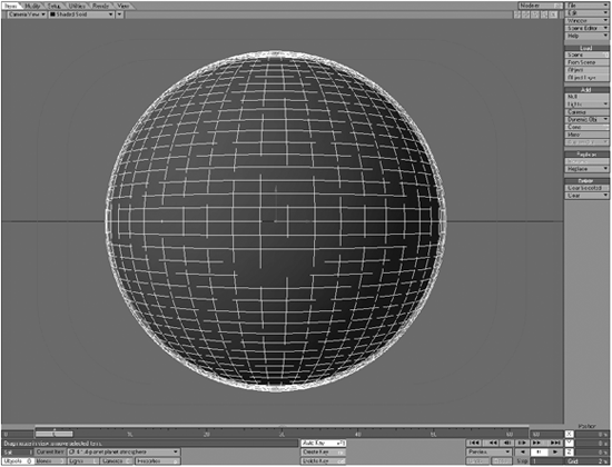
Figure 15-54

Figure 15-55
3. We want to add a little luminosity to the planet just to give its lit side a little more definition. Go back to the Surface Editor and open the planet surface’s Luminosity Texture Editor. Set up the default layer that is created as a gradient using Light Incidence as its Input Parameter. Select the light in the scene as the light that will affect the gradient.
4. Now let’s create some keys in the gradient so that we get the right look on the planet surface. Select the key that is automatically created at the top of the gradient, and change its Value to 0%. This ensures that areas that are facing away from the light will not appear luminous. Create a key at the very bottom of the gradient (make sure that the key is directly on 90.0 in the Parameter field), and change its Value to 150%. This makes the area of the planet that the light is hitting very luminous. We want the change to only happen on the very edge of the planet though, instead of a smooth transition from the nonluminous area to the luminous one, so let’s create a final key to do this. Create a key at 85.0° (check the Parameter field to ensure this) and change its Value setting to 90%. See Figure 15-56.
This gradient has now created a luminous strip along the edge of the planet that faces toward the light in the scene. It basically serves to fake the effect of extreme brightness caused by a sun on a planet as seen in space.
5. Go back to the Surface Editor and change the Diffuse setting to 40% and the Specularity setting to 5%. Leave the other settings as they are.

Figure 15-56

Figure 15-57
6. Let’s set up the planet atmosphere surface. We’ll use this part of the object to simulate an active atmosphere for the planet with the help of a few gradients.
Set up the surface’s color as 200, 120, 60. This creates a nice orange color.
7. Open the surface’s Transparency Texture Editor, change Layer Type to Gradient, and select Incidence Angle as its Input Parameter. This is because we want the atmosphere to appear transparent on top of the actual planet surface, and only have it visible along the edges in space.
8. Leave the key at the top of the gradient as it is, and make a new key at the bottom, at 90.0°. Leave this key’s settings as they are as well. Now make a key in the middle of the gradient (make sure the Parameter setting for this key is 45.0) and leave its settings as they are too. Finally, create a key in between the one you just made and the top key. Make sure that its Parameter setting is 20.0 and change its Value to 50%.

Figure 15-58
We have now created a basic atmosphere that gives the impression of a halo around the planet. To give it a little more life, we’ll quickly give it a touch of luminosity to make it a little stronger.
9. Copy the layer you just created in the Transparency Texture Editor by clicking on the Copy button and choosing Selected Layer(s).

Figure 15-59
10. Now go to your Luminosity Texture Editor and replace the default layer with the copied one by clicking on Paste and selecting Replace Selected Layer(s).
11. Essentially, the luminous aspect of the atmosphere now has the same position and falloff as its transparency, so now the entire atmosphere is glowing. The glow is a little too weak though, so invert the keys on the gradient by clicking on Invert Keys at the bottom of your gradient option to switch the effect over. The glow is now a little stronger along the edge of the planet.

Figure 15-60
We don’t want the entire rim of the planet glowing, since part of it is unlit by its local sun. Let’s make sure that the glow only appears on the illuminated face of the planet by masking this gradient layer we just created in the Luminosity channel.
12. Create a new Gradient layer above the previously made one, select Light Incidence as its Input Parameter, and choose the light in the scene from the Light list. Select the key at the top of the gradient ramp and set its Value to 0%.
13. Now create another key at the bottom of the gradient and change its Value to 100%. Change the Blending Mode of the layer to Alpha.

Figure 15-61
This now makes the gradient below this layer visible only where the light is illuminating the planet.
Render your scene; it should look like the following figure.
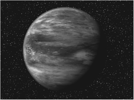
Figure 15-62
Cubic Projection
Using Cubic Projections
A cubic projection is really simple. It is basically the same as planar projection, except it does not require an axis. Instead, it takes the image map and simultaneously projects it along all three axes.
This means that you end up with the same image projected along all three axes of the model to which the surface is applied, as shown in Figure 15-63.
This projection method is particularly useful for tiling images on structures like buildings, especially if you ensure that your images are seamless. Of course, the drawback to using this particular method is that tiled textures can look a little monotonous, and if the repeating texture is very obvious, this can look quite bad.

Figure 15-63
To help break up the monotony somewhat, try using a procedural layer on top of the images with some kind of blending applied to it, so that it adds an element of randomness to the texture.
Figure 15-64 shows a Turbulence procedural applied to the surface on top of the cubic mapped image. The Turbulence adds a nice dirty look to it that breaks up the repeating pattern somewhat, and makes the overall surface more interesting.
Of course, this is a rather extreme example. You wouldn’t necessarily have to make it look so dirty! Using different blending modes (discussed in greater depth in Chapter 13), you can create a number of different blending effects.

Figure 15-64
I generally tend to use cubic projection on background elements that are never really seen in any detail and that I just don’t have the time or inclination to paint textures for. Basically, it’s the quick fix projection type.
Front Projection
Using Front Projections
Front projection is an essential part of your compositing work. It will aid you in the process of matching your CG objects to background plates. The concept behind front projection is simple: You essentially replace the selected surface with your background plate image or sequence, which is usually the same one as in the Compositing tab in the Effects panel (Ctrl+F7).
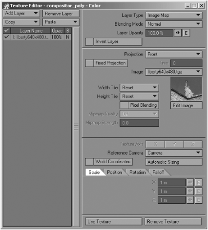
Figure 15-65: Front Projection texture
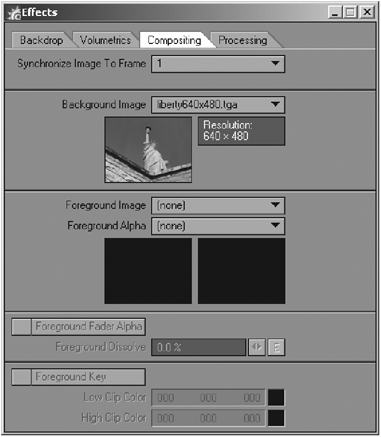
Figure 15-66: Effects Compositing tab
Front projection doesn’t “stick” the texture to the object unless Fixed Projection is on, but we’ll talk more about that in a bit. You can move, rotate, scale, and deform your object, and the texture will always face the selected camera; hence its name. The way this works is by “pin-registering” the surface image to the background, giving the impression that the CG objects in the scene are interacting with the background plate. By matching a piece of geometry to a piece of your background plate, you can create accurate shadows and reflections cast by your CG objects. You can also occlude CG objects with portions of the plate to create, for example, a UFO hovering behind a building.
It is important to note that the texture transformation options (Scale, Position, Rotation, and Falloff) are unavailable with front projection since the texture is tied to the selected camera specified in the Reference Camera pull-down menu in the Front Projection Texture options. What is more relevant to front projection is the image resolution and pixel aspect ratio. Front projection images are always the size and pixel aspect ratio as if the image were loaded as the background image, so changing the resolution and pixel aspect ratio of the camera in the Camera Properties panel (“p”) will also affect the front projection. It is best to match the camera resolution to that of the background plate used in front projection to ensure a perfect match.
Speaking of match… matching or aligning geometry to be used for the front projection is probably the most challenging part. You need to ensure that the geometry that has the front projected surface matches as closely as possible the background plate; otherwise, you might lose the effect.
Also keep in mind that you don’t want any kind of shading on your front projected objects. To correct this, set the surface Diffuse value to 0% and Luminosity to 100%. You may need to change other values for the surface, depending on what you are trying to achieve.
In the Texture Editor, when using front projection, you will see a check box to turn on or off an option called Fixed Projection. What this does is “stick” the projection of the camera. It is best to keep camera motions subtle since you can go only so far using 2D images in a 3D camera move. When you activate Fixed Projection, the Time options become active. Here you can enter a frame or time where you want the texture to be pin-registered to the background (front projected); for the rest of the frames the texture will be Fixed Projected. Figure 15-67 shows Lady Liberty getting a visit from some friends.
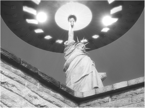
Figure 15-67