
Chapter 24
Natural Surfaces
In the previous tutorials you learned how to paint realistic organic surfaces using painting software such as Photoshop. Now we’re going to take a look at how to create natural surfaces with procedural textures and nodes. You can achieve the same results with the layer system, but nodes are more flexible. You may want to duplicate the results with the layer system in order to practice with it as well.
Natural Surfaces Tutorial 1: An Ocean
In our first tutorial we are going to create water. There are several things that you need to keep in mind while creating water. Think about the type of water you would like to create; for example, is it a pond, a river, or an ocean? All of these will look different since the surrounding environment is not the same. You also have to know what kind of weather conditions you’d like your scene to have. This will have a great impact on how the water looks. There are other variables that will affect the look of water such as nutrients, particles, sediment, and any other debris that might be found floating around. The combination of all these things will determine what the water will look like.
Before we begin, we’re going to be working with the new Node Editor shading system. We’ll be making some simple network connections that you should be familiar with if you read Chapter 14. If you skipped that chapter, I recommend you go back and read it thoroughly. There are a lot of things in the new LightWave shading system that you may not be completely familiar with, such as anisotropic shaders, diffuse shaders, and SSS shaders, to name a few. Since we are going to be focusing more on the texturing aspects of things, I have provided a complete scene on the companion CD for you to work from. If you would like to see the models, just load them up in Modeler. They are all very simple to make on your own.
The ocean that we are going to create is set in the late afternoon with medium winds that are strong enough to get some nice waves, almost like a storm is about to hit.
Load up the ocean_for_tutorial.lws scene. This scene has all the elements already placed and ready to be textured. The scene also contains a sky created with SkyTracer to be used as our background and reflection environment. You can also use your own image, preferably a panorama or an HDRI probe. This background is essential to the scene since water reflects its environment; a good reflection map will make a huge difference in your final render by providing contrast, detail, and mood to the scene. Water scenes tend to look very flat if the reflected environment is poor or has not been added to the scene at all. The NewTek web site (http://www.newtek.com) also provides some great sky photos that you can use.
NOTE: For more information on SkyTracer, consult your reference manual.
Creating the Displacement Node Network
In LightWave v9, the Node Editor can be accessed from three different places: the Deform tab of the Object Properties panel, the Volumetric Lights of the Light Properties panel, and the Surface Editor via an Edit Nodes button. In each of these instances, the Node Editor targets that specific area. We’re going to be using nodes in the Surface Editor and in the Object Properties as a displacement map.
1. Once you have loaded the ocean_for_tutorial scene from the companion CD, select the ocean and open the Object Properties panel (“p” on the keyboard).
We’re going to be using the first two tabs: Geometry and Deform. For now, we’ll leave the Subdivision Order in the Geometry tab at First; we’re also going to leave the Display SubPatch Level at 3 and set Render SubPatch to Per Object Level. Later we’ll change it to Per Polygon Level to take advantage of the new Adaptive Pixel Subdivision (APS), which will allow us to add a lot of detail to our ocean without getting a huge render hit.
2. Now go to the Deform tab; you will notice there is a button labeled Edit Nodes. Click on this button to open the Displacement Node Editor. Also click on the check box next to this button to actually activate it; otherwise, whatever we do in the Node Editor will not be reflected in the viewport or renders.

Figure 24-1: Object Properties panel
Once in the Node Editor, you’ll see the Displacement destination node. That’s the final node to which everything will be connected. Beginner- and intermediate-level users might want to try using the Node Editor to replicate what could be done using layers alone in older versions of LightWave. This will make for an easier transition. The Node Editor has dedicated Layer nodes that bring the “classic” layers of the Texture Editor into the Node Editor, making it easier to have a smoother transition to nodes (see Chapter 14, “The Node Editor,” for more on Layer nodes). In this first tutorial, we are going to follow that line of thought to make the beginning of our journey into the Node Editor a snap.
NOTE: Displacement maps are also covered in Chapter 25, “LightWave/ZBrush Workflow.”
3. Here, go to the Add Node menu and add a Scalar Layer under Layers. In this Scalar layer we’re going to add layers like we used to do in the “classic” Texture Editor. You will find this to be easier in the beginning. As your skills start getting better with nodes, you’re going to find yourself deviating from layers and instead incorporating function-specific nodes into your network.
4. Now, double-click on your Scalar layer and you’ll see a panel that resembles the classic texturing system. In this panel, we’re going to create the different types of layers that we need for our waves displacement. There should be a default layer in the node. Click on the Layer Type pull-down menu and change this layer to a procedural texture. Once you select Procedural Texture from the list, the layer is converted to a procedural texture layer with Turbulence as the default. Let’s make some changes to this texture; leave the Blending Mode as Normal, but change Layer Opacity to 20%. We don’t want the texture to be too strong. The trick here is to blend several different layers together and try to get rid of the CG-type look that we often see on images. Change the following settings for this layer:
Texture Value: 0.5
Frequencies: 3
Contrast: 0%
Small Power: 0.5
Scale X, Y, and Z: 500mm

Figure 24-2: Turbulence layer
5. Now we’ll move on to the next layer where we’ll create the larger waves. At the top-left corner of the Texture Editor, you will see a pull-down menu called Add Layer. Click on this menu and select Procedural from the list. The default is Turbulence; click on the Procedural Type pull-down menu and select Crumple, which will give a sharper top and smoother bottom to the waves. Change Layer Opacity to 55%, change Blending Mode to Additive, and also change the following:

Figure 24-3: Crumple layer
Texture Value: 2.3
Frequencies: 1
Small Power: 0.75
Scale X: 10m, Y: 2m, Z: 8m
6. Next we’ll create another Crumple layer. Change Blending Mode to Additive and Layer Opacity to 50%. Changing the opacity in a layer allows you to control the overall look of the waves and how they interact with each other, in essence controlling the size or strength of the wave patterns that they create; higher opacity values will create a more prominent wave while lower opacity values will create a more subtle wave. Here are the layer settings:

Figure 24-4: Crumple layer
Texture Value: 0.8
Frequencies: 1
Small Power: 0.75
Scale X: 8m, Y: 2m, Z: 3m
7. If you would like to animate this ocean, go to each of the layers and add an envelope. For example, let’s go to the first layer we created, the Turbulence layer on the bottom of the stack. Click on the Position tab located at the bottom of the panel. You will see an “E” button at the far right of each of the channels. E stands for Envelope, which lets us animate it. When we select the “E” button, the Graph Editor pops up; this is where we can add keys to the layer and have it animate over time. At frame 30, add a key to the Z position. Change Value to 1.5m. Change Post Behavior to Offset Repeat in the drop-down menu so it repeats over time. We will repeat this process in all the layers with a slight offset. Chapter 18, “Enveloping Basics,” has more information on the process of animating textures using envelopes.

Figure 24-5: Texture animation
8. Go to the second Crumple layer from the top of the layer stack and once again click on the “E” button. In the X position at frame 60, change Value to 3.1m, and then set Post Behavior to Offset Repeat. In the same frame but at the Y position, let’s change Value to 3.29m or something close to that and change Post Behavior to… yep, you guessed it… Offset Repeat. Change the Z position with 1.6m as Value and set Post Behavior again to Offset Repeat. By offsetting these position values we can create the illusion of movement; making some waves look big and some small, and moving at different rates gives it a more realistic look.
9. Open the first Crumple layer from the top of the layer stack and offset the values at frame 40 by creating keys on the graph just like we did before. Let’s change the X position to 555mm, Y to 333mm, and Z to 166mm. All of the channels should be set to Offset Repeat. The value is incrementally added to the original values and therefore makes it seem like it is moving for however long the animation turns out to be. After some fine-tuning, these patterns will look very nice animated.

Figure 24-6: Alpha gradient
10. Finally, we are going to add another layer. This will be a black and white gradient. Click on the Add Layer pull-down menu and select Gradient from the list. The first key should be white, with a Value of 1 and Alpha at 100%. The second key at the bottom of the gradient (the “End” value) should read 150m, with a Value of 0 and Alpha at 100%. These values will make the strongest crumple. Put this gradient between the two Crumple textures we created by clicking and dragging the gradient layer to its new location. This gradient will act as an alpha gradient, so change the Blending Mode to Alpha. The strength of the layer below it (Crumple in this instance) will start to fade toward the horizon line, ensuring that there are no visible high points on the horizon that would kill the depth effect.
11. Now let’s make all these layers work together. You will notice that the displacement is a Vector input. That is what is recommended. You can connect other inputs, but the results may vary and may be very unpredictable. In order to have this scalar layer work with a Vector input, we need to add a new node called Scale. Go to the Add Node menu and choose Math>Vector>Scale to add it to the network. You’ll notice that you have Vector and Scale inputs and a Result output. We need to tell the displacement which direction to use when calculating the map. Create a spot info node by going to Add Node>Spot>Spot Info. We’re going to take the Normal output of the Spot Info node and feed it to the Vector input of the Scale node. Then take the Scalar output of the Scalar node and connect it to the Scale input of the Scale node. This will specify how far and in which direction the displacement should be. Now that these are set up, we can connect the Result output of the Scale node to the input of the Displacement destination node. When you do that you should be able to see the ocean object displaced in the viewport.

Figure 24-7: Displacement node network
12. Close the Node Editor and go back to the Object Properties panel, then go to the Geometry tab. Now we’re going to use a feature called Adaptive Pixel Subdivision (APS), which is new in LightWave v9. As I mentioned earlier, this will let us create an incredible amount of detail in our subdivided object without a huge render hit. Change the Render SubPatch option to Per Polygon Level. Click on the “T” button to open the Texture Editor. Here we are going to set how much detail we want to see while keeping memory and render times at a reasonable level. To do this, create a gradient and change the default key Value setting to 65. Add an additional key and give it a Value of 1. In order to see the gradient working, change the End parameter at the bottom of the gradient to 10m. Now we have a gradient that starts at a value of 65 and ends at a value of 1. This will create a lot of details where we need it, right in front of the camera, and less detail where we don’t need it, farther back toward the horizon line. In order for this to work properly, we need to set the Input Parameter of the gradient to Distance to Object and select the Null object named alpha ref as the controlling object.

Figure 24-8: APS
That’s it for the displacement map. You can make a test render to see the ocean so far.
Creating the Surface Node Network
We have a good-looking wave pattern going in the scene, but it isn’t very convincing yet, is it? Let’s fix that now, shall we?
1. Open the Surface Editor (F5), select the ocean surface, and click on the Edit Nodes button to open the Node Editor. Remember to activate nodes by clicking on the check box next to the Edit Nodes button in order to see the results in the rendered image.
2. To keep things simple in this exercise we are going to use a Color Layer node and a Bump Layer node, which work just like the “classic” Texture Editor for the color and bump channels of this surface, so go ahead and add them to the workspace (Add Node>Layers>Bump Layer and Color Layer).

Figure 24-9: Incidence Angle gradient
3. Double-click on the Color Layer to open the Texture Editor; here we are going to add a couple of gradients. Set the first gradient to Incidence Angle and add two additional keys, one in the middle and the other one at the bottom of the gradient. Change the key values to the following (top to bottom):
Key 1
Color: 4, 10, 19
Parameter: 0
Key 2
Color: 14, 34, 74
Parameter: 42.6
Key 3
Color: 36, 95, 177
Parameter: 90
4. The second gradient will make the ocean a bit desaturated toward the horizon line. These two gradients set the overall color of the ocean; if you wish to change the ocean color, start with these two. Set this gradient’s Input Parameter to Distance to Camera so the color of the water will change relative to the camera position. Set the End value for the gradient to 200m or so. Here are the rest of the gradient’s values:

Figure 24-10
Key 1
Color: 1, 2, 20
Parameter: 0m
Key 2
Color: 121, 141, 172
Parameter: 200m
5. All we have left to do for the color layers is create the foam. For this, create a Dented procedural texture with these settings:
Layer Opacity: 200%
Invert Layer: On
Texture Color: 238, 244, 255
Scale: 2.46
Power: 0.806
Frequency: 0.859
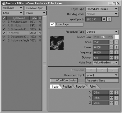
Figure 24-11: Dented layer
Noise Type: Value-Gradient
Scale X: 25m, Y: 15m, Z: 20m
6. This texture is quite large and strong in order to be seen properly; however, toward the horizon the water starts to look more like snow. To correct this, you can add an Alpha gradient that will fade the texture toward the horizon. Add a gradient layer to the stack, set the Blending Mode to Alpha and the Input Parameter to Distance to Camera, and set the End value to 200m. Add the following keys to the gradient:

Figure 24-12
Key 1
Color: 255, 255, 255 (white)
Alpha: 100%
Parameter: 0m
Key 2
Color: 000, 000, 000 (black)
Alpha: 100%
Parameter: 200m
TIP: Click and drag on the Dented texture preview to browse through the patterns. This works on all procedural textures.
7. Add another layer of foam to the ocean, making this one an FBM Noise procedural texture. This layer will add some foam specks to the water, like leftovers from a larger foam area.
Change this texture’s values to the following:

Figure 24-13: FBM Noise texture
Octaves: 4
Noise Type: Gradient Noise
Scale X: 60m, Y: 1m, Z: 60m
8. To further emphasize the look of foam, add another gradient to the layer stack to mimic the white foam on the tips of the waves. Leave its color at white and add two additional keys with these settings (from top to bottom):

Figure 24-14: Foam gradient, key 1
Key 1
Alpha: 0%
Parameter: 0
Key 2
Alpha: 0%
Parameter: 0.8
Key 3
Alpha: 75%
Parameter: 0.96
9. Now that the Color Layer is finished, connect its Color output to the Color input of the surface destination node.
10. Let’s add more detail to the waves with a bump map. Double-click on the Bump Layer node that you added earlier. Here you can add as many bump procedural textures as you wish (depending on memory, of course). What you are looking to do here is build details that would be impractical to do with displacement maps alone. First add a Turbulence texture with these settings:
Layer Opacity: 50%
Texture Value: 50%
Frequencies: 3
Contrast: 0%
Small Power: 0.61
Scale X: 3m, Y: 1m, Z: 3m

Figure 24-15: Turbulence texture layer
11. Now add a couple of Crumple procedural textures to add smaller details to the waves with the following settings:
Layer Opacity: 80%
Texture Value: 80%
Frequencies: 4
Small Power: 0.75
Scale X: 2m, Y: 1m, Z: 1m
Layer Opacity: 70%
Texture Value: 90%
Frequencies: 4
Small Power: 0.75
Scale X: 1m, Y: 500mm, Z: 500mm

Figure 24-16: First crumple texture
12. It would be a good idea to add an alpha gradient to these bump textures in order to lessen the effect of texture flickering if the ocean were animated. Add a gradient layer to the stack, set the Blending Mode to Alpha, and set the End value to 200m. Add the following keys to the gradient:
Key 1
Value: 100%
Alpha: 100%
Parameter: 0m
Key 2
Value: 40%
Alpha: 100%
Parameter: 91.2m

Figure 24-17: Second crumple texture
Key 3
Value: 14%
Alpha: 100%
Parameter: 169.3m
Key 4
Value: 0%
Alpha: 100%
Parameter: 250m

Figure 24-18: Alpha gradient, key 1
13. Since alpha gradients only affect the layer immediately below them, you need to copy this gradient and paste it on top of each of the procedural texture maps. Connect this node’s Bump output to the Bump input of the surface destination node. It really doesn’t matter when you make the connections, but it is a good idea to make connections right away if you know for sure what you are doing so you can see your changes in VIPER.
14. We need to change other channels of the surface to make the ocean more realistic. Let’s change the Diffuse channel of the surface first. In this case, add a Turbulence texture to the workspace (Add Node>3D Textures>Turbulence) and change this texture’s values to the following:
Layer Opacity: 95%
Small Scale: 0.5
Contrast: 0
Frequencies: 3
Scale X: 1km, Y: 1m, Z: 1km
15. Connect the Color output of the Turbulence node to the Diffuse input of the Surface destination node. You should have so far a Color Layer node, a Bump Layer node, and a Turbulence node connected to the surface. Don’t worry about the dissimilar type connections we made here; all we are doing is using the color information instead of the alpha information of the node to drive the diffuse value of the surface. The node network should look like the one shown in Figure 24-19.

Figure 24-19
16. You have now made a few nodes, changed values, and made connections; let’s add another element to the process. Add a Gradient node to the workspace (Add Node>Gradient>Gradient). Open the gradient’s edit panel and change these values:
Input: Incidence
Key 1
Color: 255, 255, 255 (white)
Alpha: 100%
Position: 0
Key 2
Color: 000, 000, 000 (black)
Alpha: 100%
Position: 1
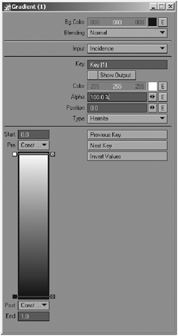
Figure 24-20: Gradient edit panel
17. Connect the Color output of the Gradient node to the Reflection input of the Surface destination node. This simulates the Fresnel effect.
18. For the Transparency channel, we can use a Surface Thickness layer to control the amount of transparency according to a specified thickness value. Since we are trying to replicate what we would usually do with the “classic” layer system we need to add a Scalar Layer node to the workspace (Add Node>Layers>Scalar Layer) and connect the Scalar output to the Transparency channel input of the Surface destination node. In this node, create a gradient set to Surface Thickness as the Input Parameter, change the End value to 400mm, and also change these key properties:
Key 1
Value: 0.85
Alpha: 100%
Parameter: 0
Key 2
Value: 0.15%
Alpha: 100%
Parameter: 400mm
19. Instead of a Specular channel we are going to use a Specular Shading channel where we can adjust the specular and glossiness properties at one time. Create a Blinn node (Add Node>Shaders>Specular>Blinn) and change the following:
Color: 255, 255, 255 (white)
Specularity: 85
Glossiness: 55
20. Connect the Color output of the Blinn to the Specular Shading channel of the Surface destination node. Done! If you render frame 139, your surface should resemble something like Figure 24-22.

Figure 24-21: Finished node network

Figure 24-22
21. Now, select the Ocean surface and go to the Advanced tab of the Surface Editor. Here, I played with the Color options on the bottom of the panel. I changed Color Highlights to 5% to add a bit of color to the highlights. I also changed the Color Filter and Additive Transparency settings to 50% each. Color Filter will tint transparent surfaces such as our ocean. Additive Transparency will add the color of the transparent surface to objects seen through it. Play with these settings to see what kind of results you get.
You can save this image or sequence and open it in a compositing or painting package to manipulate it further. In Photoshop I composited a picture of clouds that I downloaded from one of my favorite texture sites: http://www.mayang.com/textures.
I also added a layer to create haze. I first made a gray bar that goes across the horizon line. Then I blurred it and tried to match its color to the haze of the cloud picture to blend it further. The horizon line was a little too sharp, so I blurred it with Gaussian blur.
I thought it would be cute to add a couple of paper boats to the image; this will also help the viewer to better determine the size of the ocean. The Photoshop comp can be found in the companion CD if you would like to take a look.

Figure 24-23: Final composite
Summary of Tips for Creating Water
• Determine the type of environment surrounding the water body.
• Always use a good reflection map.
• Use displacement maps for low-frequency bumps (big waves).
• Use bump maps for high-frequency bumps (tiny waves).
• Gradients are your friend, and can be used for anything from color to Fresnel effects.
• Envelope every texture to give it a more realistic look when animated.
Natural Surfaces Tutorial 2: Red Rocks
The Ocean tutorial was a great exercise to get a little experience with the Node Editor. We created some simple layered nodes and plugged them in to their appropriate inputs of the Surface destination node in a way similar to what we used to surface with the classic layered system. Let’s experiment a little now with a more challenging exercise. Nice rocky terrains are difficult to create with procedurals in the classic layer system because of the number of layers needed to convincingly create such a surface and hide the “computer-generated” look that procedurals tend to have. You could easily end up with 25 color layers on one channel alone, so looking at the big picture, it would be an incredibly difficult task to make edits to this surface. With nodes you can see all of the textures of every channel at once, which is extremely helpful, but the coolest thing is to have the power to use one node to control several properties at once. For example, to reuse a gradient, you do not have to copy and paste the gradient into a different texture channel; you simply connect it to every texture you wish to affect.
Like in the Ocean tutorial, and anything else that you attempt to create, collect as many reference images as possible. Don’t just look at it, but study it and observe it. Are the shadows sharp or fuzzy? What color are they? What do you think the time of day was when the photo was taken? What’s the weather like? Is the mountain smooth or rough looking? Is it granite or sandstone? Ask yourself as many questions as possible; the answers will help you in the texturing process.
As before, the objects and scene can be loaded from the companion CD, so load the scene and let’s get to work!
About the Canyon Model
If you open the canyon_plain.lwo file from the CD you will see that unlike the ocean, I actually modeled the canyon to follow a very natural realistic pattern. I used the references I collected to model this object. The lines are based on a real-world canyon; I took creative freedom here and there, but the point is that for this kind of terrain it helps if the mesh’s edges flow realistically from the beginning. This will help our displacement map as well. This is not to say that a canyon such as this one couldn’t be done by displacing a subdivided mesh like we did with the ocean, but I find that it is more difficult and/or time consuming to do. This is totally based on personal preference. You may also create landscapes with programs such as Vue5; in this case I already had in mind exactly what I wanted, so I just modeled it.
The scene called canyon.lws that I provided for you has everything set up… with the exception of textures of course.
Creating the Displacement Node Network
1. Once you have the scene loaded, click on the canyon object and open its Properties panel (“p”). Subdivision Order should be set to First. The Render SubPatch drop-down should be set to Per Object Level and 16 and the Display SubPatch Level to 3, just so we can see a hint of what we are doing on the viewport.
2. Click on the Deform tab of the Object Properties panel, make sure the Edit Nodes check box is selected, and click the Edit Nodes button to open the editor. We are going to use some texture nodes along with some utilities and function nodes. Add a Spot Info node; by now you know that you are going to use the Normal output of this node for every displacement that you do, and the same goes for the Scale node, which is the node that combines the direction normal and the value of the textures we put together. The output result will be plugged into the input of our Displacement destination node.
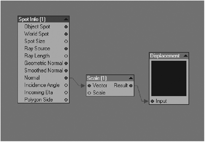
Figure 24-24: Spot Info and Scale nodes
3. Now add two 3D textures: Turbulent Noise and HeteroTerrain. Double-click on the HeteroTerrain texture to open its attributes. Change Fg Color to white and leave the rest of the HeteroTerrain attributes at their default values with the exception of the texture’s Scale, which should be X and Y: 15m, Z: 20m to stretch the texture on the z-axis. You can connect the Alpha output of this node to the Scale input of the Scale node. You should be able to see a change on the canyon object in your viewport since there is something to displace now. To make this texture more random looking, we are going to connect the Alpha output of the Turbulent Noise node to the HeteroTerrain’s Opacity input. This is like changing the texture mode to alpha in the classic layer system. Change the Turbulent Noise attributes to the following:
Opacity: 150%
Increment: 0.5
Lacunarity: 2.0
Octaves: 6.0
Noise Type: Perlin Noise
4. This texture should be somewhat bigger in order to fade large areas of the HeteroTerrain texture, so let’s change the Scale values to X and Z: 25m, Y: 2m.
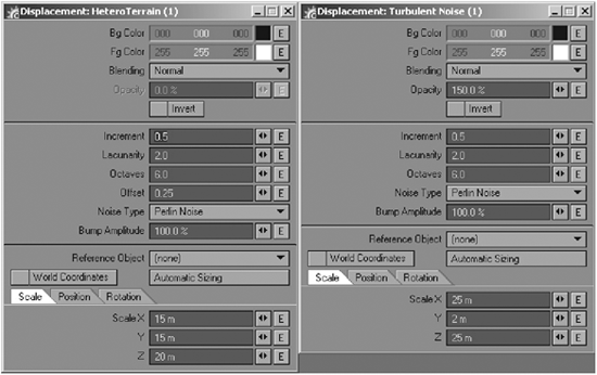
Figure 24-25: HeteroTerrain and Turbulent Noise attributes
5. So far, so good. At this point I would like to add another two-node network to this setup to add interest and detail. Add a Turbulent Noise node and a Crumple node. Double-click on the Turbulent Noise node to open its attributes and change the following values:
Increment: 0.509
Lacunarity: 1.8
Octaves: 6
Noise Type: Perlin Noise
6. Let’s make this texture stretch a little on the y-axis by changing the scale to X and Z: 5m and Y to 10m. Now let’s change where this texture shows up by connecting the Crumple texture Alpha output to the Opacity input of the Turbulent Noise that we just created. I very rarely leave textures with their default values, so scale this Crumple texture as well to X and Z: 30m and Y: 50m. Make the Background color a dark gray, 52, 52, 52. To give the crumple a more organic feel, change these attributes:
Opacity: 50%
Small Scale: 0.75
Frequencies: 2.0
7. After changing these values, make the connection, setting the Alpha output to the Opacity input of the Turbulent Noise node.
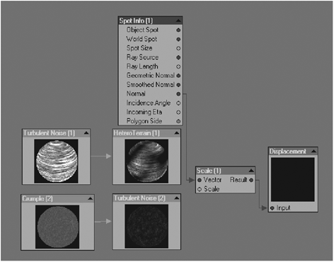
Figure 24-26: The displacement network so far
8. In order to mix these textures together, we are going to use a node called Add. This node is located under Add Node>Math>Scalar>Add. Plug the Alpha output of the HeteroTerrain to the Add A input and the Alpha output of the Turbulent Noise to the B input of the Add node. This basically reads: A+B = new value. The result of this node is plugged in to the Scale input of the Scale node. You should notice a difference in your viewport. You can make test renders after each node is configured and connected into the network to better see what you did to the canyon object.
9. Now, in order to perturb the displacement a little further we can use Function nodes, which are simply curves. The texture is disturbed according to the attributes that make the curve. Add a Noise Function node, a Modulate Function node, and a Crumple texture (you can copy and paste the texture already on the network). Open the Crumple attributes, make sure the background color is black and the foreground color is white, and type in these values:
Opacity: 50%
Small Scale: 0.3
Frequencies: 3
Scale X and Y: 15m and Z: 30m
10. Connect the Alpha output of this Crumple texture to the Amplitude of the Noise and Modulate nodes. Open the attributes of the Noise function and change the value of Clamp High to 0.5, then open the Modulate attributes and change the Frequency to 0.5 as well. Connect the Result output of the Noise function to the Function 1 input of the Modulate node. Modulate allows you to mix Function nodes together, so take the Result output of Modulate and connect it to the HeteroTerrain node Function input.
TIP: Functions should only be connected to Function inputs. Connecting functions to any other input will have unpredictable results.
11. Make a test render and see the nice rocky displacement that we have created. By changing the Opacity setting of the Crumple node attached to the Turbulent Noise, we can control the amount of displacement of the ridges that go horizontally across the surface.

Figure 24-27: Finished displacement network
Creating the Surface Node Network
We are now ready to texture the canyon’s surface. This network will be more complex than the ocean we created earlier, but there is no heavy math hocus-pocus. As your skills develop, you will undoubtedly be experimenting with more math wizardry, but for now we’ll keep things simple.
In LightWave v9 we have more diffuse shading models available to us besides the default Lambert. One of those shaders is called Minnaert, which was designed to describe nonatmospherical celestial bodies such as moons. Even though we are not making asteroids or moons, this shader will provide us with a believable surface for the canyon that is close enough to the type of surface that you might find on a moon or maybe even Mars.
1. Open the Surface Editor (F5), select the canyon surface on the list, and click on the Edit Nodes button. Make sure the check box next to Edit Nodes is active; otherwise, the changes will not be seen in the render. Once the Node Editor is opened, we will find the Surface destination node. We are going to change this default shading model to Minnaert. Add this node to the workspace with Add Node>Shaders>Diffuse> Minnaert. Open the node’s attributes and change the Diffuse value to 85%, but leave Darkening at 0.
2. We need to add some color variation to the surface to mimic the layers you would expect to see on rocky mountains. First create a Color Layer node (Add Node>Layers>Color Layer), a Crackle node (Add Node>3D Textures>Crackle), and a Mixer node (Add Node>Tools>Mixer). We are going to make a base color with these nodes and then build the color from there. Open the Color Layer node attributes and make the default layer a Turbulence procedural with these attributes (see Figure 24-28):
Blending Mode: Normal
Layer Opacity: 37.5%
Texture Color: 124, 124, 143
Frequencies: 2
Contrast: 22%
Small Power: 0.545
Scale X: 5m, Y: 20m, Z: 5m

Figure 24-28
3. Add a Gradient layer going from white to black and select Alpha from the Blending Mode drop-down menu. Also, select Weight Map as the Input Parameter and pick the “rough” weight map from the drop-down menu. Figure 24-29 shows the rough weight map. I created a few weight maps to isolate different areas of the canyon. For more information on weight maps, see Chapter 10, “Using Weight Maps for Texturing.” Open the Crackle attributes; you can leave the background color as is but change the foreground color to a dark orange like 135, 89, 3. Keep Blending Mode set to Normal and change the following properties:
Figure 24-29
Small Scale: 0.5
Frequencies: 3.0
Scale X: 5m, Y: 15m, Z: 5m
4. Now we need to mix these layers together using the Mixer node. Connect the Color output of the Color Layer node to the Bg Color input of the Mixer node and the Color output of the Crackle node to the Fg Color input of the Mixer node. Open the Mixer’s attributes and change Opacity to 17.5%. Plug the Color output of this node to the Color input of the diffuse Minnaert shader, then connect the Color output of this shader to the Diffuse Shading slot of the Surface destination node.

Figure 24-30: Base color network
5. We can now start building detail and interest to our color texture. I would like to have the Crackle texture show only in the areas designated by the “smooth” weight map. To do this, add a Weight Map node to the workspace: Add Node>VertexMap>Weight Map. Double-click the Weight Map node and select the smooth weight from the list, then connect the output of this node to the Opacity input of the Crackle node. At this point you might be asking, “Why take this route when we already have a Color Layer node and we could have added these nodes there?” The answer is because I would like to control the background color of the Crackle texture with a Crumple texture and this would not be possible with the Layer node. Add a Crumple texture to the workspace (Add Node>3D Textures>Crumple), then open the attributes of this node and change the following:
Bg Color: 84, 35, 22
Fg Color: 201, 122, 88
Small Scale: 0.75
Frequencies: 4
Scale X, Y, Z: 5m

Figure 24-31: “Smooth” weight map
6. Now take the Color output and plug it into the Crackle Bg Color input. Now the Crackle background color is driven by the Crumple texture. Cool, huh?

Figure 24-32
7. The texture is looking good, but it is lacking something very important for achieving a realistic look for a canyon such as this one… the strata, or layers that make the canyon. To do this we’ll use a gradient with several different earthy colors. Add a new Gradient node and change the End of the gradient to 25, which is about the height of the canyon. Create the following keys and spread them out almost evenly through the length of the gradient as seen in Figure 24-32:
Key 1: 70, 44, 40
Key 2: 106, 61, 44
Key 3: 95, 50, 30
Key 4: 99, 67, 48
Key 5: 172, 109, 79
Key 6: 106, 61, 45
Key 7: 158, 77, 53
Key 8: 70, 44, 40
8. After you create these keys, select the third key from the top and click the Show Output button; this will add Key Color, Key Position, and Key Alpha to the Gradient node for that particular key. Now you are able to plug in different nodes to drive that particular key’s properties. Here, we are going to drive that key’s color with a Crumple texture (Add Node> 3D Textures>Crumple). Open the node attributes and change the following:
Bg Color: 50, 31, 29
Fg Color: 139, 74, 55
Small Scale: 0.75
Frequencies: 4
Scale X: 56m, Y: 73m, Z: 90.5m
9. Now connect the Color output to the Key Color input in our gradient. You can do this for every key in the gradient and have a massive amount of detail. This is possible to do in the classic layer system, but it would consist of a massive number of layers, which could lead to a massive amount of confusion. Being able to drive keys with other textures in the network is a really powerful feature that you will be using often. To finish the color of the surface, connect the Color output of the gradient to the Color input of the Color Layer node. Make a test render and check the results. All we need now is a little bump detail to finish off the canyon.

Figure 24-33: Finished color node network
10. For the bump, we are going to take a similar approach to how we did the color textures. Add a Turbulent Noise node and an fBm Noise node to the workspace. Open the Turbulent Noise attributes panel and change these settings:
Increment: 0.5
Lacunarity: 2.0
Octaves: 6.0
Noise Type: Perlin Noise
Bump Amplitude: 35%
Scale X, Y, Z: 800mm
11. Also change the following values for the fBm Noise node:
Increment: 0.5
Lacunarity: 2.0
Octaves: 6.0
Noise Type: Perlin Noise
Bump Amplitude: 40%
Scale X, Y, Z: 300mm
12. Connect the Bump output of the Turbulent Noise node to the Bump input of the fBm Noise node. This is very similar to what we did earlier while working with the color nodes.

Figure 24-34
13. We are looking to create subtleties on the bump of the surface and break up the “computer made” look that procedurals tend to have, so let’s add a couple more 3D texture nodes and blend them all together. Add a Crumple node and a Crust node. Open the Crumple first and change these attributes:
Small Scale: 0.75
Frequencies: 4
Bump Amplitude: 15%
Scale X, Y, Z: 300mm
14. Open the Crust node’s Properties panel to change these values:
Width: 10%
Contrast: 0
Bump Amplitude: 15%
15. Leave Scale at the default 1 meter. Notice how we are changing the Bump Amplitude of every bump node; by doing this, the strength of the bump will be subtle, as we are not looking to overpower the look of the image with a very strong bump. The last two nodes are meant for the ground. There is a weight map already created in the canyon object for this purpose; all we have to do is add a Weight Map node with the ground weight selected from the node’s attributes panel and plug that in to both the Crumple and Crust nodes’ Opacity inputs.
16. We can control the value of the ground weight a little better by adding a gradient to the network. Add a Gradient node (Add Node>Gradient>Gradient) and make this gradient go from white at the top to black at the end. Connect the Value output of the weight map to the input slot of the gradient, then connect the gradient’s Color output to the Opacity of the Crumple, Crust, and Turbulent Noise nodes’ Opacity inputs.
17. Since bumps are vector in nature (XYZ), the Mixer node won’t do such a good job, so we need a different way to combine these together to be able to connect all the nodes to the Surface destination node Bump input.
One way to do this is with an Add node, which is available as a scalar and/or vector (Add Node>Math>Vector>Add). Now connect the Bump output of the fBm Noise node to the A input of the Add node, and plug the Bump output of the Crust node to the B input of the Add node; the result output can finally be plugged in to the Bump slot in the Surface destination node.
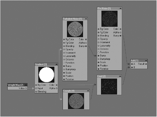
Figure 24-35: Bump node network
18. To finish it off, you can add a CookTorrance specular shader and plug it in to the Specular Shading slot in the Surface destination node, and bring the Glossiness setting down to 5%.
Make a new render to see the results. From here you can experiment by adding more color and bump variation using the techniques that you followed here and see what you come up with. Figure 24-37 shows the final composite in Photoshop; I created a screened bloom layer and added some adjustment layers to do some minor color corrections.

Figure 24-36: Finished surface network
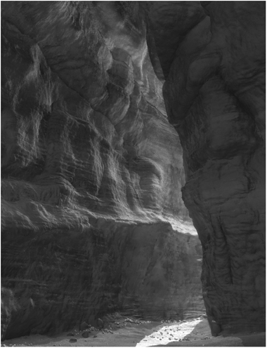
Figure 24-37: Final composite
Summary of Tips for Creating Canyons and Rocky Mountains
• Study as much reference material as possible; this goes for anything you do.
• Have a clear knowledge of the type of rock that makes the canyon or mountain.
• Make the Bump Amplitude of nodes small and adjust from there; subtlety is key.
• Remember that the colors of the strata will change depending on the type of rock that makes the terrain.