
Chapter 14
The Node Editor
The Node Editor is a new and extremely powerful tool for texturing and shading in LightWave. Node-based texturing systems have been the standard in the industry for a while and are far superior to layer-based systems like the “classic” Texture Editor, which is restrictive and can be difficult to edit content with. A node is basically a data holder if you will. This data holder can be linked to other data holders forming a network of nodes passing data to each other. This network of nodes is represented on the computer as a flow chart very similar to the schematic view in Layout.
Even though this might seem very technical and a departure from layers in LightWave and Photoshop, you will see that it is extremely powerful and easy to learn. The Node Editor is easy enough for beginners to get great-looking surfaces, and powerful enough for the advanced user using heavy math to make some incredible shaders previously impossible to achieve in LightWave. With the new LightWave Node Editor you do not lose the capability of using layers either; on the contrary, it is enhanced, since it has “Layer” nodes specifically made for this purpose. You can also work with both environments simultaneously, so if you have color layers already built in your surface using the “classic” layer system but you wish to change the Diffuse shader and add subsurface scattering (SSS) to your surface with nodes, you have the power to combine the two texturing systems so the color layers don’t have to be rebuilt.
Before we begin looking at all the different nodes available to us (of which there are quite a few), let’s study the Node Editor interface and some basic usage concepts that you need to be familiar with to make understanding this incredible system a snap.
Getting to Know the Node Editor
The Destination Node
The Node Editor in LightWave v9 is located in three different places, each of which is dedicated to a specific task: surfacing, displacements, and volumetric lights. The greatest difference between these is what is called the destination node. We are going to be concentrating on surfacing, but the same concepts apply to displacements and volumetric lights. The destination node is simply the master or root node of the surface network; it contains all the surface property inputs that make that particular surface, such as Color, Diffuse, Specular, etc.
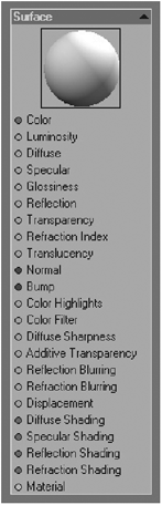
Figure 14-1: Surface destination node
The Node Editor Interface
Let’s take a quick look at the Node Editor interface, which is actually very simple to navigate and use.
Open the Surface Editor and click on the Edit Nodes button to launch the editor. On the far left you will see a drop-down menu called Add Node. In this menu you select the nodes you would like to add to the workspace. This menu can also be accessed by pressing and holding Ctrl+Right Mouse Button anywhere on the workspace area. Next to the Add Node menu is the Edit drop-down menu. This menu contains functions such as Rename, which allows you to rename the node, as well as Copy and Paste, Select All, and Invert Selection. Other options that you will find useful are Export Nodes and Import Nodes. With Export Nodes you can select a group of nodes and save them for future use. All the connections of those nodes and their relative locations will be saved as well; however, the destination node will not get exported nor the connections made from the saved node network to the destination node. Import Nodes opens a file requester where you can select the .node file to be imported to the current Node Editor, so you can interchangeably use saved node networks between surfaces, displacements, and volumetric lights.
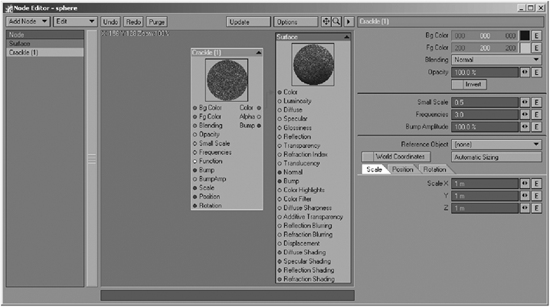
Figure 14-2: The Node Editor interface
The Edit menu also has a Preview submenu, from which you can select what you would like to see in the Surface ball of the node if one is available. Some of the preview options are: Color, Alpha, and Bump. Other options may be available, depending on the type of node you have selected. The Edit menu can also be accessed with a shortcut; select the node on the workspace and right-click on it to get to the whole Edit drop-down menu right on the workspace. To the right of the drop-down menus you have the standard Undo and Redo buttons followed by a Purge button. This button gets rid of all of the Undo history in memory.

Figure 14-3: Drop-down menus and buttons on the left side of the screen
At the top right of the screen there is a button called Update. This button forces the Node Editor to refresh all of the Preview balls of the nodes in the workspace. The Options button, which is the same as the options in the Surface Editor, lets you change the size of the Preview Surface ball, the background, and the refresh method (Auto or Manual). Next, you see widgets for panning and zooming, and another one to collapse or embed the Node Edit panel. If you decide to collapse it, the Node Edit panel will display a floating panel. This is how I personally use it since I like to have more real estate open for the workspace.
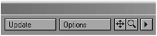
Figure 14-4: Buttons on the right side of the screen
Below the buttons are two large areas. On the left is a Node list column, where you can see all the nodes you have available on the workspace. On the right you have the workspace, where you make all your node connections. Below the workspace is a Comment area, where you can type in comments to describe something or to give directions.
Right on the workspace you will see a node already there waiting for you. This is the destination node that I talked about earlier. This is where you connect nodes in order to create the final look of that particular surface.
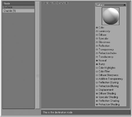
Figure 14-5: Node list, workspace, and Comment area
Connection Types
Now this might be a bit boring, but it is absolutely essential for you to know just what all these connection types are all about. After all, how on earth are you supposed to create beautiful shaders if you have no idea what the connections are actually doing? So let’s look at the destination node, where you can see all the attribute slots that make the surface. Notice that these inputs are color-coded; these colors give you a visual cue of the type of connection that is recommended for that particular attribute.
There are six different types of connections in the Node Editor: Color (red), Scalar (green), Vector (blue), Integer (purple), Function (yellow), and Material (cyan). These connections are described below.
Color Connections (Red)
Color is probably the easiest connection type to understand since the data that it outputs is simply red, green, and blue values (RGB). You will most likely want to plug color attributes to color inputs; however, there might be times when you will want to plug dissimilar types of connections to color inputs. In these instances the incoming data will be converted and fed to each of the RGB channels. If the incoming data is a scalar value, that same value will be fed to each RGB channel equally. On the other hand, if the incoming input is a vector (position, rotation, or scale), then the position and scale X value will be connected into the Red channel, the Y value will be fed to the Green channel, and Z to the Blue channel. For rotation, the heading value will be connected to the Red channel, the pitch value will be connected to the Green channel, and the bank value will be input to the Blue channel.
Scalar Connections (Green)
A scalar is a floating-point number, so it can be either positive or negative (such as 5, 80.55, or −30.66). A Scalar connection holds one value at a time, as opposed to connections such as Color, which holds three values (RGB), or Vectors, which hold three values as well (XYZ or HPB). Since scalars can only hold one value at a time, if you make dissimilar connections, then the Node Editor makes a conversion and not all the data will get used. In the case of Color connections, the Node Editor will convert the RGB values to Luminance and use that instead. In the case of a Vector connection, only the first value will be used, such as X if it is position or scale and H if the vector is rotation.
Vector Connections (Blue)
In the most simplistic description, Vector designates direction in the form of position (XYZ), rotation (HPB), or scale (XYZ). Vectors are necessary for bump maps, normal maps, and displacement maps, to name a few. For example, without a vector, the surface won’t know in which direction you wish to apply a bump map and thus the results would be unpredictable. You can make dissimilar connections to Vectors, but like Functions, all the data might not get used or it might give unpredictable results. If you connect a Color output to a Vector input, the RGB values will be fed into the XYZ or HPB values, respectively. Remember that when making dissimilar connections, if the connection is Scalar or Integer, the same value will be used in all three channels.
Integer Connections (Purple)
Integer connections are whole numbers, usually to tell a node to pick an item from a list, such as blending modes. You might be asking yourself, “Why would I need to use a node to select the blending mode of a node?” Well, if you have a simple network you can just open the node and do it manually, but what if you have 10 nodes that use the same blending mode? Then you would use an Integer node to control all 10 blending types of those nodes at once, which is a very efficient way to handle this type of situation. You can also make connections of dissimilar types with Integer connections, but just like Scalars, not all the data is put to use; for example, Color connections will use the Luminance value rounded to the nearest whole number of either 0 (black) or 1 (white). In other words, if the Luminance value is above 50%, the integer will be 1; if the Luminance value is lower than 50%, then the integer will be 0. If the dissimilar connection is a Vector, then just like with Scalars, the only value used is the first one, either X for position and scale or H for rotation; the other values are discarded.
You can reference the following table to find the correct integer for any of the blending modes available along with a brief description.
Table 14-1: Blending modes
Number | Description |
0 | Normal. This option doesn’t transform the textures at all. This is the default value. |
1 | Additive. Adds the values of Bg Color to the values of Fg Color. |
2 | Subtractive. Subtract the values of Bg Color from the values of Fg Color. |
3 | Multiply. Multiply the values of the Bg Color with Fg Color, thus darkening the texture. |
4 | Screen. This is basically the inverse of Multiply. The result is always a lighter color blend of the Bg Color and Fg Color inputs. |
5 | Darken. Uses the darkest texture values as the result; lighter values get replaced. |
6 | Lighten. Uses the lightest texture values as the result; darker values get replaced. |
7 | Difference. This is similar to Subtractive but uses the difference of values instead of their subtraction. |
8 | Negative. Has the same effect as Difference. |
9 | Color Dodge. The Bg Color is evaluated and the Fg Color brightens in a similar way as Screen, but colors tend to get saturated as well. |
10 | Color Burn. This option is similar to Multiply; the Bg Color is evaluated and the Fg Color darkens as a result. Colors tend to get saturated as well. |
11 | Red. The red channel from the Fg Color input is used, and the green and blue channels from the Bg Color are used for the color output. |
12 | Green. The green channel from the Fg Color input is used, and the red and blue channels from the Bg Color are used for the color output. |
13 | Blue. The blue channel from the Fg Color input is used, and the red and green channels from the Bg Color are used for the color output. |
Function Connections (Yellow)
Functions are graphs that are able to transform a texture or shader value. Always connect Function outputs to Function inputs. Making dissimilar connections with functions is not recommended since results are unpredictable. Functions work as a two-way communication between the connected nodes, so data is sent to the function, it gets transformed, and then it is sent back to the connected node.
Material Connections (Cyan)
Material nodes help you in the process of simulating physically accurate materials such as metals (conductors) and glass (dielectric), among others. They are color-coded in cyan. I recommend making similar connections when using Material nodes for more predictable results.
Making Connections
It is recommended for beginners to make connections that belong to the same category; however, the Node Editor is flexible enough to allow dissimilar connections to be made. When this happens, the connection type is automatically converted, but in some cases not all the data is used. For example, connecting any other type of output to a Function input will yield unpredictable results. As your skills develop, you will find instances where making dissimilar connections not only makes perfect sense but sometimes is necessary, so when the time to make dissimilar connections comes, don’t be afraid to do so and experiment. There are just a couple of things that you need to remember when making dissimilar connections in your network: You can only plug Vector connections to the Normal and Bump slots of the destination node and only plug Function outputs to Function inputs. For now, let’s stick to similar types of connections and get comfortable using and navigating through the Node Editor.
Connecting nodes is actually quite simple; just click on the output and drag the arrowhead to the input you wish to plug to. To disconnect, click and release the arrowhead. Simple, right? When you make a connection of similar types, the connection line between the nodes will be the color of that particular type; for example, for a Color output to a Color input the line will be red, for a Scalar output to a Scalar input the line will be green, and so on. If you make a connection of dissimilar types, the color of the line will change from the color of the output to the color of the input. This is a great way to tell visually that the connection is of dissimilar types.
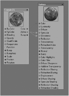
Figure 14-6: Nodes connected
Let’s make a couple of connections to get you comfortable with this concept.
1. Load the know_the_node_editor.lws scene file from the TutorialsNode Editor folder on the companion CD.
2. Activate VIPER (F7) and make a render (F9) to save the buffer for VIPER.
3. Open the Surface Editor (F5) and turn on the Node Editor by clicking on the check box, then select the plane surface and click on the Node Editor button to open it.
We have the destination node there waiting for us to connect some nodes to it. We are going to make a simple dirty floor texture, so click on the Add Node button and add a Turbulence2D node (Add Node>2D Textures>Turbulence2D). This is going to be the dirt layer of the dirty floor.
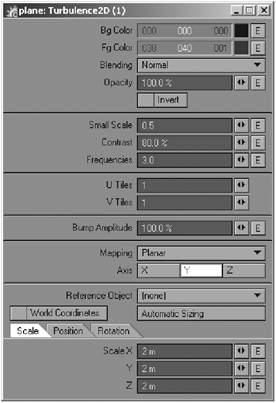
Figure 14-7
4. Click on the node to see the attributes in the Node Edit panel if it is embedded on the Node Editor interface. If you have decided to collapse the embedded panel to gain more real estate, then double-click on the node to open the Node Edit panel as a floating panel. Once opened, change the following attributes (see Figure 14-7):
Fg Color: 38, 40, 1
Small Scale: 0.5
Contrast: 80%
Frequencies: 3
Mapping: Planar
Axis: Y
Scale X, Y, and Z: 2m
5. Now, grab the Color output of the node and plug the arrowhead to the Color input of the Surface destination node.
VIPER should update, showing large greenish and black tones on the floor. Congratulations! You have made your first node connection.
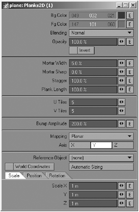
Figure 14-8: Planks2D texture
6. Okay, let’s add some detail to this rather boring texture. Add a Planks node (Add Node>2D Textures>Planks2D) and change the following attributes of this node:
Bg Color: 49, 32, 21
Fg Color: 147, 101, 60
Mortar Width: 5.0%
U and V Tiles: 5
Bump Amplitude: 200%
Mapping: Planar
Axis: Y
7. Connect the Color output of this node to the Bg Color input of the Turbulence2D node.
Once again, VIPER updates after the connection is made, showing us a planks pattern with disgusting green dirt on top.
8. Change the UV Tiles values of the Planks node to see how this affects the pattern. I ended up leaving it at 5 tiles.
9. Let’s add some texture to the planks to make it look more like actual wood (Add Node>3D Textures>Wood) and open the Node Edit panel to change some of its attributes.

Figure 14-9: Wood texture
Bg Color: 198, 162, 101
Fg Color: 181, 89, 1
Opacity: 80%
Frequencies: 3
Turbulence: 2
Ring Spacing: .0.05
Ring Sharpness: 3
Axis: Z
Scale: X, Y, and Z: 3m
10. Connect the Color output of this node to the Fg Color of the Planks2D node. Now you see in VIPER that the planks have a woodgrain pattern.
11. Now I would like to break up the dirt layer. To do this add a Crumple texture to the workspace (Add Node>3D Textures> Crumple), and open the Node Edit panel to change the following:
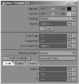
Figure 14-10: Crumple texture
Small Scale: 1.0
Frequencies: 3
12. Now, right-click on this node, choose Preview, and select Alpha. The sample ball will update to show the alpha output of the node.
13. Connect the Alpha output of the Crumple texture to the Opacity input of the Turbulence2D node. You will see in VIPER that the greenish dirt layer’s opacity is now driven by the alpha output of the Crumple texture. Very cool!
14. Change the Diffuse value of this surface since as you already know nothing is 100% diffuse; there is always light absorption, even if it is very little (Add Node>Constant>Scalar). Change the Scalar value to something like 0.85, and connect it to the Diffuse input of the Surface destination node.
15. Now take the Bump output of the Planks2D node and connect it to the Bump input of the Surface destination node. Also take the Alpha output of the Turbulence2D node and connect it to both the Specular and Glossiness inputs of the Surface destination node.
Make a test render to see the results. Your dirty floor is finished. Notice that all the connections are of similar types.
One thing that I really love about surfacing in the Node Editor is the ability to see every texture for every attribute of the surface at once. Before, in the “classic” Surface Editor, you would have to open each attribute by clicking the “T” button in order to see what made that particular attribute. You could not have the Color and Bump texture editors open at the same time. Another thing I absolutely love that you will find extremely useful is the ability to connect outputs of nodes to several different inputs at the same time, thus having the control of changing several properties with one single node or output.
Consider this scenario: In the classic Surface Editor you have 50 different color layers, and each layer needs an alpha layer to control the opacity of each color layer. This approach is tedious to edit as you would have 100 layers total (yes, I have done textures this complicated before), not to mention that you also need the same alpha for the diffuse and specular channels. With the Node Editor you can have just one alpha node controlling everything, including the color, diffuse, and specular layers. Just edit one alpha node and everything updates automagically!
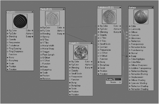
Figure 14-11: Finished node network
By now you should feel pretty comfortable making connections and getting around the Node Editor. Figure 14-12 shows the result of the node network that we just created for the floor. As an exercise, go ahead and texture the sphere that is sitting on the floor on your own and see what you come up with. Start with easy networks and build detail from there; try to replicate what you could do with the “classic” layer system.

Figure 14-12
Next we are going to review the built-in nodes available in the Node Editor.
LightWave v9 comes with a great library of nodes built in for you. The LightWave v9 SDK also allows you to build your own nodes; if you happen to be a coder, that is. Here we are going to go through the nodes included with LightWave, some of which you might be familiar with since they are available in the form of layers in the “classic” Texture Editor. The vast majority, however, are new textures or utilities that you might not have heard of before. Let’s review these textures in a linear fashion from top to bottom as they appear on the Add Node pull-down menu. Also, for illustrative purposes, any image of the nodes presented will be applied to the Color input of the surface unless otherwise noted. Keep in mind that the basic concepts of procedural textures as described in Chapter 8 are still applicable.
2D Textures
2D Textures are either procedurals or image maps that can be mapped to objects using common projections such as Planar, Spherical, Cylindrical, or UV maps. LightWave will project the textures realistically on objects with basic geometric shapes such as planes, spheres, cubes, etc. Another advantage of using these 2D procedural textures is that they are 100% tileable; just enter the number of tiles you wish the texture to have and LightWave will do the rest. If you happen to find some unexpected errors in your images, such as artifacts or completely blurred textures, try turning Mip Mapping off; this is the usual suspect when render errors like those come up.
Bricks2D
The first texture in the 2D Textures list is Bricks2D. This texture is pretty much the same as in the classic Texture Editor with the exception that all of the attributes that designate the texture are available as inputs, so these attributes can be driven by other nodes in the network. Let’s take Fg Color for example. This attribute can be driven by the color that makes a Crumple texture in order to give color to the bricks. The Bg Color input will color the mortar of the bricks, and also can be driven by other nodes in the network. You can also connect nodes to Mortar Width and Mortar Sharp in order to make the bricks irregular shapes. Remember that if the value of Mortar Width is too high, the mortar will completely cover the bricks. A couple of inputs that are available in this node that its layer cousin lacks are the U and V Offset values. With these inputs you can plug other nodes into the network to offset the texture and provide you with a different look; Figure 14-13 shows the result of plugging a Crumple texture into the U Offset value.
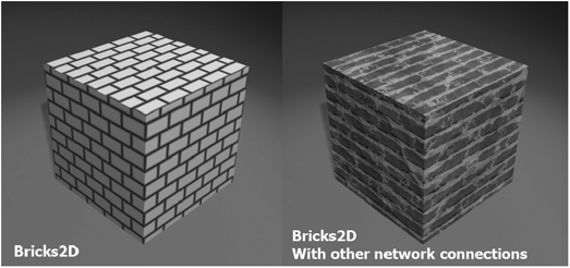
Figure 14-13: Bricks2D with nodes driving different attributes
NOTE: Refer to Chapter 8 for more information on the Brick procedural.
Other inputs that most textures have are the Bump and Bump Amplitude inputs. Bump designates the bump of the surface, while Bump Amplitude designates how strong the bump will be. Try not to connect dissimilar types to these inputs unless you absolutely know what you are doing. By plugging the Bump output of other nodes into the Bump input, you are able to mix bumps together, as shown in Figure 14-14.

Figure 14-14: Connecting Bump output to Bump input
CheckerBoard2D
Guess what this node does! All joking aside, this node will be useful if you are making any type of texture that requires a checkerboard pattern. Yes, you can make chessboards with this, but think of other possible uses this node can have, such as stainless steel tiles in a kitchen, wallpaper coverings, fabrics, and more. Think outside the box. This texture will also come in handy if you want to quickly check for texture stretching in your UV maps. This texture, as with most 2D textures, needs a projection axis, whether it is Planar, Spherical, Cubic, UV, etc. Also, as with Bricks2D, you can offset the UV tiles, thus opening the door to more possibilities of what you can do with this texture.
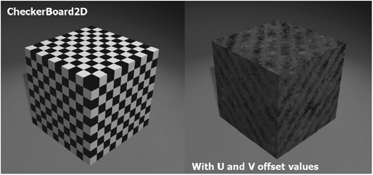
Figure 14-15: CheckerBoard2D texture
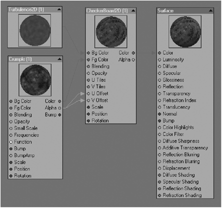
Figure 14-16: The node network
Strangely enough, this texture doesn’t have a Bump input or output, therefore limiting its potential uses.
Grid2D
This texture is very similar to Bricks2D, but the tiles it creates are arranged in perfect vertical and horizontal lines as opposed to a stacked and staggered pattern. This node is very easy to understand. The Bg Color input describes the mortar, and the Fg Color input describes the tiles. Mortar Width determines the thickness of the lines that make the grid, while Mortar Sharp determines the sharpness of the lines. This is a very useful node if you want to make tile for a bathroom, for example.
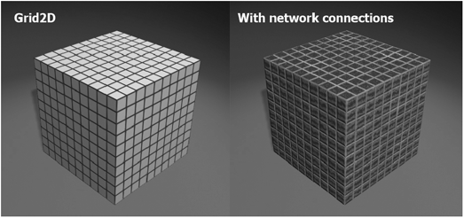
Figure 14-17: Grid2D texture
Also remember that all of these textures can serve as masks. You can make these tiles really large and the lines very thick and plug other textures into the Bg Color and Fg Color inputs to make some interesting textures.
Image
You will likely use this node quite often. Here you specify an image available in your scene or you can load one from disk using the Node Edit panel. Image is also an axial texture, so it needs to have an axis specified, such as Planar, Spherical, Cylindrical, Cubic, or UVs in the Node Edit panel. Images are extremely powerful in the Node Editor since you can drive the attributes of other nodes using an image.
Make sure you read Chapter 11, “Image Maps,” for more information on the creation and usage of image maps. This node also has Bump input/outputs and Bump Amplitude inputs so you can mix different bumps together.
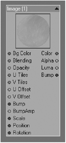
Figure 14-18: Image node
NOTE: See Appendix B for a list of file formats that can be imported into and exported from LightWave.
Normal Map
Normal Map uses a technique similar to bump mapping that adds detail without adding more polygons to your geometry, but unlike a bump, which modifies the existing normals (the direction a polygon is facing) of a model, a normal map will replace these normals entirely. Normal maps are also based on RGB values instead of the one color that a bump map is able to use, and thus saves more information than a regular bump map. In other high-end 3D applications, a network of utilities is needed in order to use normal maps; in LightWave it is as simple as loading your map and connecting its Normal output to the Normal input of the destination node.
If you work with ZBrush, this is the node you will need in order to use the normal maps that were generated with ZBrush from a high-resolution mesh.
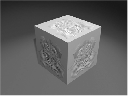
Figure 14-19: Normal mapped cube
NOTE: For more on using normal maps generated in ZBrush, refer to Chapter 25, “LightWave/ZBrush Workflow,” in Part 7 of this book.
If you open the Node Edit panel of the Normal Map node, you will see three check boxes under the Edit Image button called Invert X, Y, and Z. With these buttons you can invert the normals for that particular axis to give the impression that the detail is coming from a different direction. In Figure 14-20 I inverted the normals of the y-axis and thus made it look like the detail is a relief instead of an emboss.
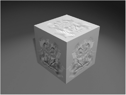
Figure 14-20: Inverted Y Normal Map
Parquet2D
Parquet is another simple node to figure out. Parquet is the pattern that you will find most commonly on wood floors. This texture, like Bricks2D, has Mortar Width and Mortar Sharp inputs so you can control the thickness of the virtual grout. One input that you will find useful is Tiles, in which you can specify the number of tiles to put on each block. If you specify one tile, then the result will be like the Grid2D node. Just like any other 2D texture, Parquet2D is also an axial texture, so you need to specify a texture axis for the projection of the texture to the object.
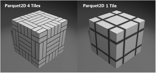
Figure 14-21: Parquet with four tiles (default) and one tile
Planks2D
You should already be familiar with this node, as we used it for the first exercise in this chapter. Very similar to Parquet2D with the exception of its pattern, this texture is mostly used to create floors, but with a little imagination you can come up with other uses. This node offers inputs to change the Stagger and Length settings of the planks.

Figure 14-22: Planks2D texture
Turbulence2D
This node is very similar to its 3D texture cousin. Turbulence2D combines different layers of fractal noise to create complex and interesting patterns. This texture is axial in nature like the other 2D texture nodes. Since this is a 2D texture node, the image is tileable. The higher the number of tiles, the smaller the pattern will get in order to fit within the number of tiles specified. The Frequencies input determines the level of detail within the pattern. Small Scale in the classic Surface Editor is called Small Power here. This value determines the amount of change between the transition of large detail and small detail areas of the pattern.
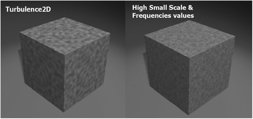
Figure 14-23: Turbulence2D texture
Turbulence2D is one of those textures that has many different uses, from dirt and grime to scratches and rust. The possibilities are limited only by your imagination.
3D Textures
If you read Chapter 8, “Procedural Textures,” you will know that 3D textures are computer generated, but unlike procedural 2D textures, 3D textures follow the geometry as if it had volume. One great advantage of procedural 3D textures is that you don’t have to worry too much about axial projections since for most they are not needed. For those few that do require an axis, it is very simple to set up since it works in a similar fashion to the 2D textures discussed above.
Also remember that these textures are for the most part identical to the procedurals in the classic Texture Editor, with the exception of some attributes available as inputs so they can be driven by other nodes in the network.
Bricks
This texture produces, well, bricks, and just like any other texture node, the attributes of this texture can be driven by other nodes in the network, thus making it possible to come up with interesting textures other than the average brick pattern. Think outside the box.
By opening the Node Edit panel you will see the attributes that make the texture. The top part of this and every other 3D texture node has to do with the colors, blending method, and opacity. Just like 2D textures, the attributes can be driven by other nodes in the network. In the second section of this panel you will find a couple of options specific to this texture: Thickness, which should really be named Mortar Thickness, controls the thickness of the mortar between the bricks, and Edge Width controls the bevel of the brick edges. Notice that these options can now be animated.
You also have options to control the Scale, Position, Rotation, and Bump Amplitude (Strength). These settings are found across the board for all textures and can also be animated.
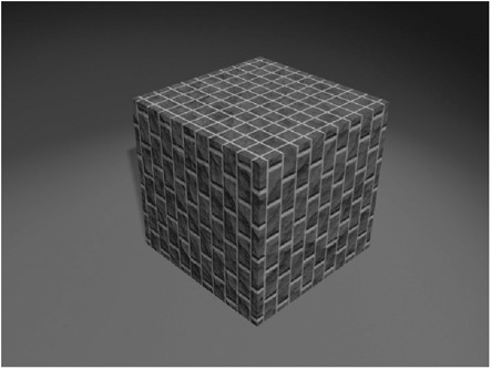
Figure 14-24: Bricks texture with a Crumple bump
Checkerboard
Well, just like the 2D Checkerboard, think of other possible uses this node could have besides chessboards. By connecting other nodes to the different attributes you can come up with some interesting effects previously impossible to achieve. I hope a Fuzzy Edge option is added in the future to make this texture even more useful.

Figure 14-25: Checkerboard texture
Crackle
This is one of my favorite textures for creating natural and organic looking surfaces due to its cellular pattern. You can create a great variety of surfaces like dried mud, lava, and even small rocks!
The Node Edit panel shows all of this texture’s attributes, and like before, the top part has to do with colors, blending mode, and opacity. The blending modes are listed in Table 14-1 near the beginning of the chapter. The middle section of the Node Edit panel has some options to control the look of the Crackle pattern: Small Scale, which determines the amount of change between detail levels of the pattern, and Frequencies, which is the actual amount of detail contained in the pattern. This option is also known as Octaves in the “classic” Texture Editor.

Figure 14-26: Crackle texture

Figure 14-27: Crackle small rocks
Crumple
This is probably the second most useful procedural, topped only by Turbulence, in my opinion. This texture can be used for water, rocks, ground, skin, leather, and organic objects (such as neurons) at the microscopic level, to name a few. Like the other textures, this node can receive inputs from other nodes in the network. The options are very similar between these 3D textures; you can change the look of the texture by changing Small Scale, Frequencies, and the various transformations such as Position and Scale.
In Figure 14-28 I made some minor changes to the Small Scale and Frequencies settings, and I also inverted the texture and changed the scale to provide the beginnings of a skin texture. Be sure to see the Ocean tutorial in Chapter 24 to see how I put the Crumple texture to work in the creation of water.

Figure 14-28: Crumple texture as bump
Crust
This texture is really great for bump maps; you can create pimples and warts, and you can even use it for creating speckles on rocks or snow. A couple of attributes unique to this texture are Width and Contrast. Width controls the diameter of the circles, and Contrast controls the fuzziness of the circle’s edges, so the higher the contrast, the sharper the circles. Two options that are not available in this node that the layer counterpart has are Ledge Level and Ledge Width; these options are covered in the Crust section of Chapter 8. I really don’t know why these two options are not available in the node, but if you absolutely need them you can still use a Layer node and add the Crust layer there.
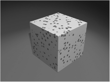
Figure 14-29: Crust texture
Dots
This node simply creates a grid of circles. I have used this texture for fabrics, wall coverings, metal grates, and other textures that require an even pattern of circles.

Figure 14-30: Dots texture
FBM
FBM stands for Fractional Brownian Motion. This texture is great for the creation of natural textures and is also great for bump maps in particular to add a general unevenness to the surface. This texture can receive attributes from other nodes in the network. As with the many other 3D procedurals we have covered, this one also has Small Scale and Frequencies settings, in addition to a Contrast setting. Just by applying the texture using the default settings you can see right away that it has a marble type of look to it, which is useful for several different things.
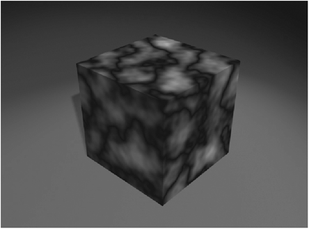
Figure 14-31: FBM texture
Grid
This texture creates a procedural grid pattern. This texture is useful for the creation of textures that require a square pattern, such as kitchen and bathroom tiles.
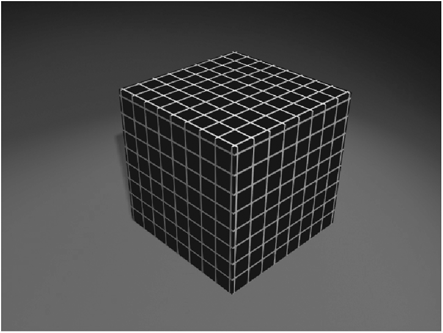
Figure 14-32: Grid texture
HeteroTerrain
This is a multi-fractal texture that works best in bump maps and displacement maps, since it simulates the naturally occurring pattern of how land tends to be flatter and smoother in valleys and rough and uneven in peaks. There are a couple of texture attributes whose terminology is different compared to other nodes, but they perform the same job. Lacunarity determines the amount of scale of the successive levels of details in the fractal pattern. Octaves set the number of levels of detail used by Lacunarity. Increment sets the strength between the layers of details. The layers are overlaid on top of each other in order to add detail to the texture. Offset determines where the combined results of the previous three options begin. You also have a pull-down menu with different noise types to pick from; some of those noises have a noticeable hit on render times with Sparse Convolution as the most expensive of the pack.
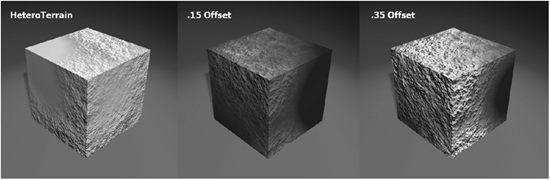
Figure 14-33: Different Offset values
Honeycomb
This texture requires a projection axis. It is great for metal grilles, fabrics, and sci-fi looking patterns if it is stretched and deformed.
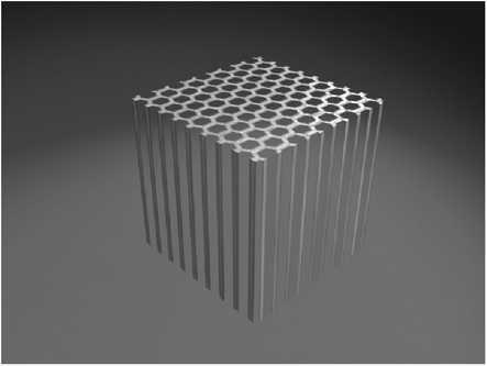
Figure 14-34: Honeycomb texture
Hybrid-MultiFractal
This texture is very similar to HeteroTerrain since it works best in bump and displacement maps for the creation of terrains. Also like HeteroTerrain, the valleys tend to be smooth while the peaks tend to be rougher, and it also shares the same types of options covered for HeteroTerrain.
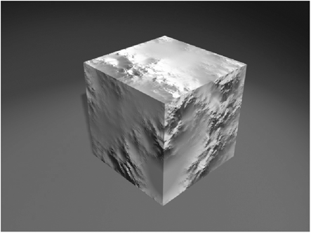
Figure 14-35: Hybrid-MultiFractal texture
Marble
This procedural texture creates fractal patterns to mimic the patterns found in marble. It is also one of the few textures that requires a projection axis to specify which axis to wrap the texture around. The attributes unique to this texture are Vein Spacing, which controls the spacing between veins within the pattern itself, and Distortion and Noise Scale. Noise Scale sets the size of the noise, while Distortion sets the amount of noise that is applied to the veins of the texture. In the “classic” Texture Editor, Marble has an option called Vein Sharpness. In the Node Editor, this option is simply called Contrast, which does exactly the same job by setting how fuzzy or sharp the vein edges are. By connecting functions you can expand the possibilities of this texture.
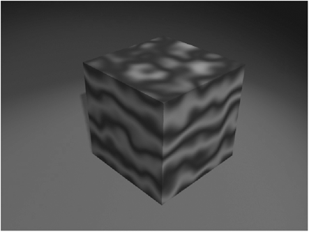
Figure 14-36: Marble texture
MultiFractal
This is yet another multi-fractal texture that is most useful for bump maps to add a general coarse look to surfaces such as rust, sand, rocks, etc. The options in this texture are the same as the other multi-fractal textures already covered.

Figure 14-37: MultiFractal rust
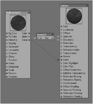
Figure 14-38: The rust node network
RidgedMultiFractal
This multi-fractal texture is most useful for bump and displacement maps to create terrains. The options in this texture are the same as the other multi-fractal textures already covered with the exception of Threshold. By increasing this value you increase the number of ridges in the texture.
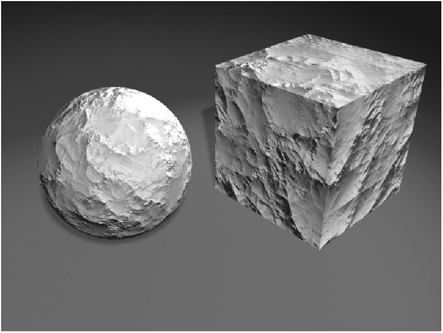
Figure 14-39: RidgedMultiFractal with different scale values
Ripples
This texture is also particularly useful for bump maps since it simulates the ripple patterns found on the surface of water. Ripples is covered in detail in Chapter 8, but here is an overview of its attributes. The Wave Sources value determines the number of sources that create the ripples; high values create lots of ripples while low values create fewer ripples. Wavelength determines the size of the space between ripples, and Wave Speed controls the speed of the ripples as they travel outward from the center of the source. Notice that all of these options in this node, unlike the layer counterpart, can be animated.
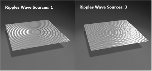
Figure 14-40: Different Wave Sources values

Figure 14-41: Different Wavelength values
Turbulence
This is probably the texture I use the most as it is extremely versatile and can be used for tons of different kinds of surfaces, from walls and rust to micro bumps and natural surfaces. The attributes that make this texture are the same as in many other 3D textures: Small Scale and Frequencies, with the addition of a Contrast input.
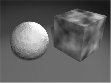
Figure 14-42: Turbulence applied as bump and color
Turbulent Noise
This is another noise texture that can be used for many different things. The attributes that makes this texture are the same as in many other textures in this category.
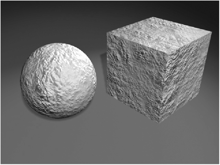
Figure 14-43: Turbulent Noise texture
Underwater
This texture is used to replicate the pattern caused by refracted light through bodies of water, which is called caustics. You can see this phenomenon at the bottom of swimming pools, for example. The attributes of this texture are similar to those of Ripples with the addition of Band Sharpness, which works like a contrast control, dictating how soft or sharp the bands look. As in Ripples, all of these attributes can be animated.

Figure 14-44: Underwater texture
Veins
This procedural texture creates patterns similar to spider webs; it is useful for creating cracked dried mud or cracked old paint, for example. You can control the Width and Contrast of the veins in this texture. Width controls the thickness of the veins, while Contrast controls how sharp (or fuzzy) the veins are.

Figure 14-45: Veins texture applied to color and bump
Wood
As mentioned in Chapter 8, this texture is similar to Marble but the pattern is meant to mimic the concentric rings found in wood. The attributes that makes this texture tick are also covered in Chapter 8 since its layer counterpart is the same; regardless, here is an overview of the attributes.
Frequencies controls the level of detail within the texture. Turbulence determines how close the wood rings are from one another as a whole. Ring Spacing controls the space between rings within the pattern itself, and Ring Sharpness controls how soft the edges of the rings are.

Figure 14-46: Wood texture and Turbulence for bump

Figure 14-47: The node network for Wood
Wood2
This procedural also has the ability to mimic wood rings in a similar way to Wood, with the exception that it allows you to phase or move the transition gradient of the rings and thus randomize the look of the rings. Like the other procedurals, you can animate the attributes of this texture so you can come up with some funky animations.

Figure 14-48: Wood2 and a Crumple for bump
fBm Noise
This node is very similar to FBM with the exception of some options unavailable in FBM. The options for the variation of pattern and detail in this texture are Increment, Lacunarity, and Octaves. The terminology of these options is different from other 3D textures but they really do the same thing. Increment controls the fractal dimension of the texture pattern, Lacunarity is the same as Small Scale, and Octaves is the same thing as Frequencies. This node, in its Node Edit panel, has a pull-down menu from which you can select the type of noise to be used in the texture, so you can create very different looks by just changing the Noise Type setting.
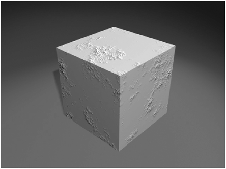
Figure 14-49: fBm Noise texture
Constant
Constant nodes simply hold a fixed value that can be used to drive and/or control other nodes’ attributes in the shading network. A couple of good examples of Constant nodes would be connecting a Scalar constant to the Specular and Glossiness inputs of the destination node, or using the Integer constant to drive the blending mode of several textures at once. These are just a few examples of what you can do with these nodes.
Angle
This node has no inputs, only an output. You can enter a value in the form of degrees to drive angular properties. You can enter values beyond 360 degrees if you need to. The Angle output of this node can also be animated.

Figure 14-50: Angle node
Color
This node is known as the Value procedural in the “classic” Surface Editor. This node simply holds color information. You can use the Color output of this node to drive the Color input of other nodes in the network from one spot; if you have created a complex shading network to create a red clay ground shader and then the art director decides to make it gray, instead of going node by node changing color values, just add this node with the new color and plug it into the input color of every node that needs to be changed. To quickly go back to the red clay color, just unplug the node and you are done.
Figure 14-51: Color node
Direction
With this node you can change the direction vector of different direction inputs, which is especially useful when you need to change the direction (heading, pitch, or bank) of several nodes, in a single place instead of manually changing the values of each node individually.
Figure 14-52: Direction node
Integer
This node is usually used to select items from a list such as blending modes or several nodes at the same time, as mentioned earlier in this chapter. You can also use this node to change the number of UV tiles in a texture.

Figure 14-53: Integer node
Pi
The value of Pi is 3.14159. Pi is defined as the ratio of a circumference of a circle to its diameter. I haven’t run into a situation where I have had to use this node, but when the time comes, I know where to find it.

Figure 14-54: Pi node
Scalar
Here you can type a value, positive or negative, to drive several different inputs of nodes such as Diffuse or Refraction Index.

Figure 14-55: Scalar node
Functions
Functions have their own connection type; try to connect Function outputs to Function inputs to avoid any problems. Functions are graphs; the node that the function is attached to gets transformed according to this graph. You can drive the different inputs of these nodes with other nodes in the network.
Bias
This function can control the brightness levels of the node that it is connected to.
For all functions, the Frequency input determines how long it takes for the function to finish one cycle. Amplitude controls the size of the function.
Throughout all function nodes you will see a couple of inputs called Clamp Low and Clamp High. What these mean is that if the graph value exceeds this number, the graph gets clipped so it doesn’t go above (Clamp High) or below (Clamp Low) the entered value. The Phase input allows you to shift the graph in time, right or left. If you open the Edit panel for this node, you will find a Mode pull-down menu that contains three options: Constant, Repeat, and Oscillate. These options control the graph after one cycle has been completed, just like the Post Behavior in the Graph Editor. Constant keeps using the value used at the end of the first cycle. Repeat repeats the graph cycle from the beginning, thus making a sawtooth pattern. The Oscillate mode causes the graph to cycle backward to its starting position and start over, sort of like ping-pong for graphs.
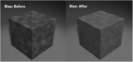
Figure 14-57: Bias before and after
These options are available in every function node in the Node Editor and are also animateable so you can create some really interesting textures.
The Bias input controls the actual bias of the function. This input can have a value from 0 to 1, with 0.5 being “normal” or the default value. Changing this value up or down will output more or less bias, respectively.
BoxStep
This function creates a box step graph so you end up with flat peaks and valleys between two values. By using this node and tweaking the Clamp Low and Clamp High values, you can control how much detail of a texture you can see and how intense it is.
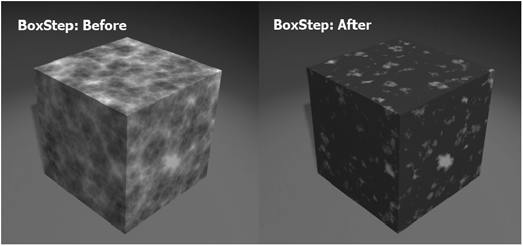
Figure 14-58: Isolating detail using BoxStep
Gain
Gain is similar to Bias, but Gain controls the contrast of textures instead of the brightness. All of the options are the same with the exception of Gain at the bottom. This option controls the overall contrast of the function. Just like Bias, 0.5 is the default value; increasing or decreasing this number will increase or decrease the amount of contrast.
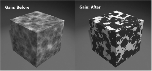
Figure 14-59: The result of Gain
Gamma
Gamma is a curve that defines luminous values in images. The Gamma node collectively controls both the Bias and Gain of the texture it is connected to. The Gamma control in the Node Edit panel can go above the value of 1 but not below the value of 0.

Figure 14-60: The Gamma node at work
Modulate
With Modulate you can combine two different functions together, which opens the door to even more interesting possibilities. The two functions are combined via different modes that are similar to some of the blending modes for color inputs of texture nodes. The blending modes are as follows:
• Add: Adds the input of function 1 to the input of function 2.
• Subtract: Subtracts the input of function 1 from the input of function 2.
• Multiply: Multiplies the inputs of both functions.
• Maximum: The output is the highest value of the two functions.
• Minimum: The output is the lowest value of the two functions.

Figure 14-61: Node network using Modulate
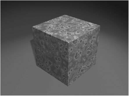
Figure 14-62: Modulate in action
Noise
This is a standard Perlin Noise function used to perturb the pattern of the texture it is connected to. Easy enough, right? This node doesn’t have the mode options that most functions have. Since it is based on a Perlin Noise, the end value will be different as you increase the Frequency input or shift it in time using the Phase input. Figure 14-63 shows an FBM texture with a Noise function.
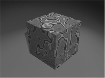
Figure 14-63: FBM texture with a Noise function
Sine
Sine allows you to regulate the transition of the texture it is connected to based on a wave-like function. The options on the top section of this node’s Edit panel are the same as the other function nodes: Frequencies, Amplitude, Phase, and Mode.
SmoothStep
This node is very similar to BoxStep with the exception that the curve is smoothed. If you find that your transitions are too sharp using BoxStep, use this node instead; it yields better, smoother transitions. Load the Smooth-Step surface from the Surface PresetsLW9 Texturing folder on the companion CD to compare the subtle difference between SmoothStep and BoxStep; just make a render of the two and switch between them to see the difference.
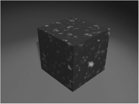
Figure 14-64: SmoothStep on a Crumple texture
Wrap
This node allows you to modify a Scalar input with a function. This is useful because you are not constrained to the Function input. This node will be very useful to you if you happen to be using math nodes with Scalar outputs in your network.

Figure: 14-65: Wrap node used as a mask with Ripples3d
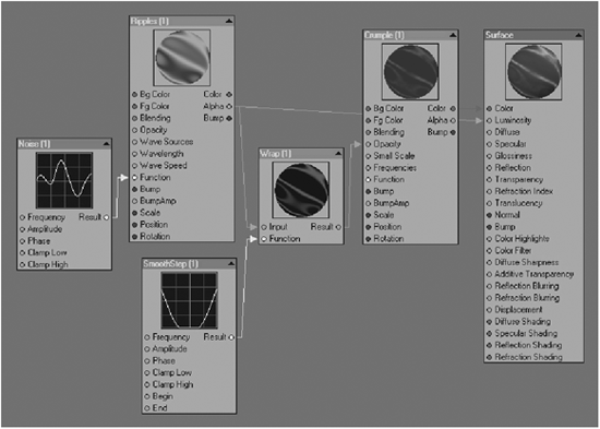
Figure: 14-66: Wrap node network
Gradients
Ah, the almighty gradients! As discussed in Chapter 9, a gradient is a graphic way to represent a graph so it is easier for us to understand the effect of this graph on the surface. Gradient nodes in the Node Editor are a bit different from the gradient layer in the “classic” Texture Editor due to some new functionality that is not available in its layer counterpart; this is discussed further in the node descriptions below. In addition to the Gradient node, you also have a couple of dedicated tools available to quickly add an effect to your network.
Tools
Incidence
This is a dedicated gradient that allows you to change the look of a surface based on the camera viewing angle. The part of the surface that faces the camera directly is at an angle of 90 degrees by default. The advantage of using this node over a gradient with the input parameter set to Incidence Angle is that in the Node Edit panel you have the option to have the angle at 90 or 180 degrees. What if we could change the actual direction of the Incidence effect? This can be done with the Vector input; you can connect the Vector output from other nodes in the network to change the direction of the Incidence effect. For example, you can drive the Incidence Angle with a light. Figure 14-67 shows the 90° and 120° Incidence options; notice the sharp black rim on the 120° image is gone. This is followed by a gradient being driven by the direction of a light in the scene; notice that the intensity of the reflection is controlled by the alpha of the gradient. See Figure 14-68 to see how this was set up.
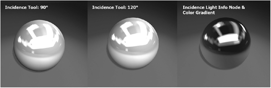
Figure 14-67: Incidence tool settings
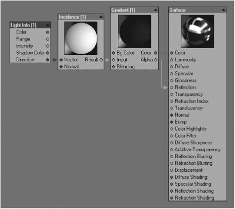
Figure 14-68: Incidence node network with a gradient
Thickness
The Thickness node evaluates the length of the ray hit point to the back of the object where the ray exits. Since this node uses rays to determine length, it is necessary to have at least one of the ray-tracing options on in the Render Globals panel. There are two inputs in this node: IOR (Index of Refraction) and Normal. The IOR input value determines how much the ray is refracted or bends; the Normal Vector input allows you to change the direction of the rays that are fired back. This node works perfectly with colored glass and water by connecting the Length output to a gradient’s input so the color of the glass is based on its thickness while using the gradient’s colors, as seen in Figure 14-69. Figure 14-70 shows the node network. Some of these node connections might not make too much sense right now, but it will become clearer as you keep reading.
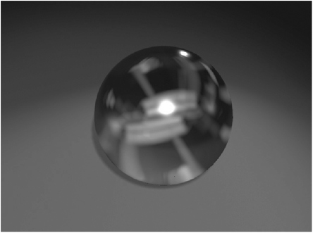
Figure 14-69: Thickness using the gradient’s colors

Figure 14-70: Thickness node network
Gradient
The Gradient in the Node Editor has more functionality than the Gradient layer in the “classic” Texture Editor. One of those new improvements (and a big one too) is that nodal gradients can be animated! The attributes that can be animated are Background Color, Color, Alpha, and Position of the keys. At first glance the node’s inputs are similar to those of other color nodes; you have Bg Color where you can connect (preferably) color attributes from other nodes in the network, or you can also enter RGB values manually via the Node Edit panel. There is also an Input slot where you can connect other nodes’ attributes to drive the gradient. What exactly does that mean? Well, it means that the gradient itself can be transformed by the connected input. Let’s say that you have a Crumple texture and a color gradient. You can connect the alpha of the Crumple to the input of the gradient to perturb the gradient based on the alpha value of the Crumple. (See Figure 14-71.)
The Blending Integer input is used to select the blending mode that will be used to blend the gradient with the Bg Color input. This list of inputs can grow according to the gradient’s keys, which we’ll discuss further in a little bit.
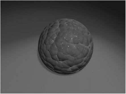
Figure 14-71: Crumple driving a gradient
Let’s study the Gradient’s Node Edit panel to see all of the options. At the top of the Gradient Node Edit panel you will find the usual Bg Color input, where you can manually enter an RGB value or connect attributes from other nodes in the network. You also have the same Blending pull-down menu, just like any of the other nodes we have covered. Now to the really cool part, the actual gradient! You create keys on the gradient by clicking on the spot where you would like to drop a key. Then you can change the color, alpha, and position of that particular key. Notice the “E” (envelope) button, which means you can animate the color of that key over time, its alpha, or its position. Just above the Color attribute is a check box labeled Show Output. When activated, this little gem will add Color, Position, and Alpha to the node; you can do that to every key on the gradient if you want. By doing this you are able to change the color of each key with any kind of texture! You can have an earth strata effect in no time with a different texture in each layer. I’ll show you how to do just that in the Red Rocks tutorial in Chapter 24. With this technique you can easily blend a number of images together by just connecting their color output to a particular key color input.
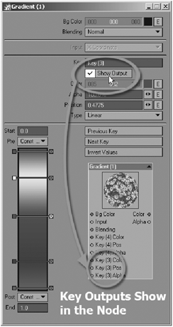
Figure 14-72: Gradient node key outputs
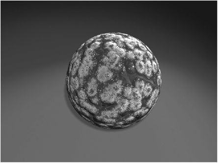
Figure 14-73: Driving key inputs
Deleting gradient keys is just as easy; just click on the little square with the “x.” If you wish to lock the key, then right-click on the little colored square on the left side of the key to change the square into an “x” (see Figure 14-74). You will no longer be able to move it; however, you can still make other kind of edits such as changing its color or alpha.
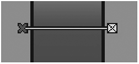
Figure 14-74: A locked gradient key
You also have buttons to navigate through the keys and a button to invert the values of the gradient as a whole. Another cool feature of the nodal gradient is the Pre and Post behaviors. The default is Constant, which means that the color of the first and last key will remain the same along the length of the gradient. If they are set to Repeat, the gradient will repeat along the length with the settings entered in the Start and End boxes. For example, if you have a mountain that is 100 meters tall you can type a value in the End box to make the gradient the same height as the mountain. If you create a gradient with the default values of 0 to 1, and set the End value to Repeat, the gradient from 0 to 1 will repeat 100 times.
Gradients are extremely versatile and you will be using them quite often in your texturing work.
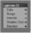
Item Info
These nodes provide you access to information about the specific item selected in the Node Edit panel. This allows you to create textures based on information provided by the items you have selected. The information changes according to the type of item you intend to use. Cameras and lights have their own dedicated nodes, which provide specific information related to cameras or lights. The Item Info node provides information regarding the selected object from the pull-down menu, such as position and rotation.
Camera
This node provides you with the settings of the camera selected in the Node Edit panel.
Item Info
Item Info allows you to select items in the scene, such as objects, lights, cameras, or nulls. It outputs vector information including world position, scaling, rotation, etc.
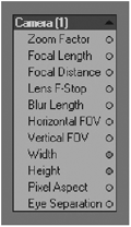
Figure 14-75: Camera node
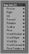
Figure 14-76: Item Info node
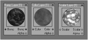
Layers
The Layer nodes allow you to integrate the “classic” layered texturing system of LightWave previous to version 9. This is a great way to get both seasoned and beginner LightWave users introduced to the new “nodal” texturing system at the same time. There are also some procedural textures that are not yet available as nodes, such as Dented. Even though you can create similar looks and effects using other texture nodes, functions, and clamps, it would still be nice to have it available as a node. In the meantime we can access them through the Layer nodes. Layer nodes are available as color, scalar, and vector types, so you can make similar connections. By double-clicking on the node you will see the “classic” Texture Editor where you can add layers and mix them together to achieve the look that you are after. For more on the Texture Editor, see Chapter 13, “The Texture Editor.”
Bump Layer
With this node you can build a stack of layers that can be connected to the Bump input of other nodes in the network or directly to the Bump or Normal slots of the destination node. This node provides a Bump input where you can plug the bump of other nodes in the network into the background bump of the Layer node. The output of this node is vector which, as you know, has X, Y, and Z components. The alpha of this Bump Layer node is available as a Scalar output and is acquired by using the intensity of the last layer on the stack.
Color Layer
The Color layer node is identical to the Bump Layer with the exception that its output type is color (RGB). You can connect dissimilar types but not all of the information will be used.
Materials
What if you run into a situation where a client hands you a book with some data sheets of the physical properties of aluminum, for example, and asks you to replicate it in the current pre-vis project? No, don’t pull your hair out; just use Material nodes. These Material nodes can help you simulate physically accurate materials. This is especially useful when matching live action plates or for artists in the science and medicine fields, where accuracy is extremely important. It is recommended that you make similar type connections to the destination node for more predictable results. Material nodes can be considered a bit advanced, but don’t let that stop you — experiment!
Conductor
This node is used to simulate physically accurate metals. Materials that can transfer electricity, heat, or both are conductors; metals are excellent conductors. This node can receive data from other nodes in the network or by manually inputting values via the node’s Edit panel. The Advanced tab of the node’s Edit panel resembles the Environment tab in the Surface Editor. Here you can select the Reflection mode you wish to use in that particular material, just like in the Surface Editor Environment tab. Remember that the use of Reflection Blur will increase your render times, so use it with caution.
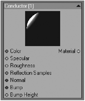
Figure 14-79: Conductor node
Delta
Delta is an energy conserving material, which simply means that the sum of Specular and Diffuse will always equal 1. For example, if you change the node’s Specular value to 40%, then Diffuse will equal 60%. In case of a Specular value of 100%, the Diffuse value will be 0%.
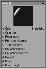
Figure 14-80: Delta node
Dielectric
This node is used most commonly for materials like glass and liquids where the index of refraction (IOR) changes according to the different materials that the rays travel through, such as air to glass to air or air to glass to liquid to air. These are just a couple of possible scenarios where this node might be useful. Dielectric uses Snell’s law to calculate refraction angles and Beer’s law to calculate absorption. It’s important to note that for this node to work properly, Double Sided should be on and Spot Info may be necessary in order to give a different IOR to both sides of the polygons being evaluated.

Figure 14-81: Typical glass network using Dielectric node
Make Material
This node is quite versatile. It allows you to make materials out of the various Shader nodes. You can also input values via the node’s Edit panel.
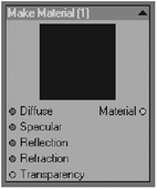
Figure 14-82: Make Material node
Material Mixer
Material Mixer is very similar to the Mixer tool, with the exception that it is designed to mix, well, you know… materials. The amount of mixing is controlled by an Alpha input, which can be manually set or controlled by other nodes in the network.
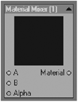
Figure 14-83: Material Mixer node
Standard
Standard replicates the built-in shading model of LightWave found in the Basic tab of the “classic” Surface Editor. When you open the node’s Edit panel you will find an Advanced tab, which mimics the Environment tab of the Surface Editor with added options such as Reflection and Refraction Blurring. This is useful when you need to create layered shaders or when using the Transparency and Refraction Index options to create glass and liquids.
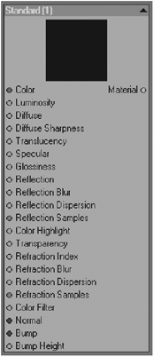
Figure 14-84: Standard node
Switch
You can compare Switch to the Logic node since you can use it to assign different properties to both sides of a polygon. This is very useful for creating glass, liquids, and any other semi-translucent material. Remember that your surface has to be double sided, and the Polygon Side output of the Spot Info node has to be connected to the Switch input inside the Switch node in order to assign different materials to the polygon sides correctly.
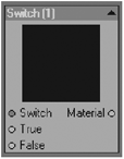
Figure 14-85: Switch node
Math
We are artists, not coders. What the heck is this math doing here!? As I said earlier in this chapter, the Node Editor is easy enough for beginners and intermediate users but also powerful enough for the advanced math geniuses out there. I won’t delve into math too much; however, there are nodes here that at some point or another you will have to use in order to mix nodes together, and maybe eventually you might want to jump into more advanced things such as trigonometry… gulp!
The Math nodes are divided into three subcategories, making it easier to find the particular operation that you would like to use by its type. The subcategories are:
• Scalar: The input and output of these nodes are always scalar values.
• Trigonometry: Trigonometry, or trig for short, is an area of mathematics that deals with angles and triangles.
• Vector: Vectors involve the concept of direction (XYZ or HPB).
Some nodes are repeated between Scalar and Vector, with the exception being the type of input they receive, which is the same type of output they produce. In other words, Scalar math nodes only input and output scalar values from and/or to other nodes in the network. Trig nodes are all Scalar, but they are separated into their own subcategory for organization purposes.
Scalar Subcategory
Abs
Absolute values are always positive or 0, never negative, so this node will convert a negative input value to a positive value. In other words, the absolute value of 350 and −350 is 350.
Add
This node adds the value of input B to input A. You can enter this value manually or it can come from other nodes in the network. The result of the addition can be connected to other Scalar inputs. This is a very useful node since you can use it for blending textures together.
BoxStep
This node basically clamps or limits the input according to the Begin and End values using a BoxStep function. Therefore, if the value of the input is smaller than the Begin input, the output will be 0.0. If the value of the In input is higher than the End input value, the output will be 1.0. If the value of the In input is in between Begin and End, the changing values transition proportionally using a box step ramp.
Ceil
Ceil, short for ceiling, rounds a scalar value to the closest whole number. For instance, if the input value is 1.3, the output would be 2.
Clamp
Clamp will limit the input according to the Low and High input values, so the output cannot go below or above (respectively) the specified values.
Divide
The value of B is divided by the input of A.
Floor
The opposite of Ceil. It will round the input value but will use the lowest integer instead of the highest, like Ceil. For example, if the input value is 5.9, the output will be 5.
Invert
This node inverts the input value, so 0.0 would become 1.0 and 1.0 would become 0. In other words, the input is subtracted from 1.0. For example, if the input value is 0.9, the output would be 0.1.
Logic
The Logic node is an IF statement. Conditions can be selected from the pull-down menu; if the condition is met, then the node will use the appropriate output as specified. The node evaluates the input information and then performs an action according to the selected condition. You can select from the following conditions: A equal to B, A not equal to B, A greater than B, A less than B, A greater than or equal to B, A less than or equal to B. In the IF inputs you can enter values or have the values be driven by other nodes in the network. This node can be used alongside the Spot Info node so that you can create double-sided objects with different IOR (Index of Refraction).
Max
Max will evaluate the inputs and will output the larger of the two.
Min
Just like Max above, but it will output the smaller of the two inputs.
Mod
Mod (short for modulus) will evaluate A and B and output the remainder of A divided by B. For example, if the input of A is 5 and the input of B is 3, then the Mod result would be 1.
Pow
I’m still trying to find a practical use for this node, but I know that the coders out there are already thinking of ways to use it.
Sign
Sign converts the incoming value of the input to its opposite sign, so a negative value becomes positive and vice versa. For example, −50.56 becomes 50.56.
SmoothStep
This is similar to BoxStep, with the exception of having a smooth ramp.

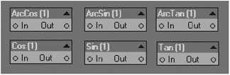
Trigonometry Subcategory
ArcCos
This node outputs the inverse cosine of the input.
ArcSin
This node outputs the inverse sine of the input.
ArcTan
This node outputs the inverse tangent of the input.
Cos
This node outputs the cosine of the input. Cosine is defined as the ratio of the side next to a given angle to the hypotenuse.
Sin
This node outputs the sine of the input. Sine is defined as the ratio of the side opposite a given acute angle to the hypotenuse.
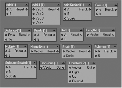
Vector Subcategory
Add
Unlike scalars, vectors have component outputs in the form of XYZ. This node will add the values of input A: XYZ and input B: XYZ respectively, so the Result output would be: AX + BX, AY + BY, and AZ + BZ.
Add4
This node allows you to add four different vectors. Since vector values are component (XYZ), the Result output of X is the sum of all four X values; the same goes for Y and Z.
Add Scaled
Similar to Add, with the exception that after the addition is finished the result is multipled by the Scale input value.
Cross
Cross calculates the Result as the product vector perpendicular to both the A and B inputs.
Distance
The output of this node is the distance between input A and input B. For example, with this node you can calculate the distance of an object to the camera or light.
Divide
This node will divide the corresponding individual component input values of A and B respectively, so the Result output would be AX / BX, AY / BY, and AZ / BZ.
Dot
Dot calculates the cosine of the angle between two vectors.
Length
This node calculates the length of a vector and outputs the result value as a scalar.
Multiply
This node will multiply the corresponding individual component input values of A and B respectively, so the Result output would be AX × BX, AY × BY, and AZ × BZ.
Normalize
This node calculates the length of all three vector components and then divides each vector value by its length.
Scale
Scale simply multiplies each vector component by the value in the Scale input.
Subtract
This node will subtract the corresponding individual component input values of A and B respectively, so the Result output would be AX − BX, AY − BY, and AZ − BZ.
Subtract Scaled
Similar to Subtract, with the exception that after the subtraction is finished the result is multiplied by the Scale input value.
Transform
This node will allow you to transform the input vector between world and object coordinates and vice versa. The Node Edit panel has a Type pull-down menu that lets you select either Object to World or World to Object.
Ray Trace
RayCast
This node allows you to cast or “fire” a ray from any position in the scene. The position is derived from the vector Position input of the node. The ray will travel in the direction taken from the Direction vector input. It will keep traveling through the scene until it hits another surface; if no other surface is hit, the result value will be −1.0. The length of the distance traveled will be the output of the node in the form of a Scalar output.
RayTrace
RayTrace works like RayCast above, with the exception that when the ray hits another surface, that surface is evaluated as well and the result is kicked back as the Color output. The Position and Direction have to be world coordinate inputs. If no other surface is hit, the resulting Length value will be −1.0.

Figure 14-89: Ray Trace nodes
Shaders
Shaders allow you to change the default Lambert shading model used in LightWave. By changing this shading model we can change how light interacts with an object’s surface and therefore we are able to create more realistic surfaces.
At the bottom of the destination node you will see four color type (red), entries: Diffuse Shading, Specular Shading, Reflection Shading, and Refraction Shading. LightWave includes several shading models for each of these properties. So what’s the difference between these and the Diffuse, Specular, Reflection, and Refraction scalar (green) entries at the top of the destination node? This question comes up very often in discussion forums. The difference is that shaders allow you to change the default Lambertian diffuse and Blinn specular models with something else altogether, while the scalar ones simply allow you to add detail using textures. They define which areas of the surface are more diffuse or more specular, for example. Shaders are organized in subcategories to make them easy to find.
Diffuse Subcategory
Lambert
This is the default diffuse shading model in LightWave. This model diffuses the reflected light evenly in all directions. This shader is especially good for plastics and high-gloss materials in general.
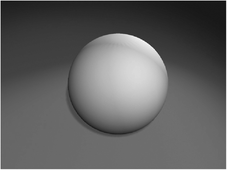
Figure 14-90: Lambert
Minnaert
This model was developed to describe nonatmospherical terrain surfaces such as the Moon and so it is also known as a “moon shader.” In this Node Edit panel you are able to pick from two implementations of the shading model; Minnaert-A is great for porous surfaces such as moons, dirt, rocks, and stone; Minnaert-B is great for fibrous surfaces such as fabrics. The Canyon tutorial in Chapter 24 uses Minnaert-A as the diffuse shader. In the Edit panel you can also play with an option called Darkening. Increasing this value to high levels will invert the surface shading.

Figure 14-91: Minnaert
Occlusion
Occlusion or Ambient Occlusion, also known as “dirt map,” is a shading model that gives you a way to add realism to your images by taking into account how light is blocked from surfaces. The result is the darkening of such surfaces as objects get closer together (and hence the name dirt map). Ambient Occlusion is not limited to reacting to objects getting closer together; it also affects its own geometry at the same time, which is called “self-shadowing.” This is great for creating images with soft shading, similar to the shading in a radiosity render without the huge render times. Of course this only affects shading, so bounce lighting is not calculated. This node can be used in many different and creative ways; the output can be connected to different node attributes in the network in order to achieve several different looks. There are just a few options to control the look of this shader: Samples, Mode, and Maximum (max).
Samples determines the number of directions a surface evaluates in order to calculate the occlusion solution. So the higher the number, the better the quality, and therefore the longer it would take to render. I tend to use 2 × 6 for test renders and 4 × 12 for final renders, although Occlusion tends to need more samples to get a smoother result.
Mode gives you two options: Infinite, which simply means that the rays have no limited range, and Ranged, which means that you can set an amount to limit the length of the evaluation rays.
Max determines the amount to be used by the Ranged mode.

Figure 14-92: No AO, Infinite, and Ranged
Since Occlusion uses rays to determine the occluded areas, Ray Trace Shadows needs to be on in the Render Globals panel for this node to work as expected. In the examples above, I connected the Occlusion node to the Diffuse Shading slot of the destination node.

Figure 14-93: Occlusion II node
Occlusion II
Occlusion II is very similar to Occlusion, with the biggest difference being a Color Mapping option in which you can select a spherical map, light probe, or background image from disk. If you use a light probe image, the Pitch option can be accessed along with Heading, which is available for every color mapping option.
OrenNayar
This shading model was designed as an improvement to the Lambertian model. It is especially good for recreating rough, matte surfaces such as clay and fabrics. The Roughness setting simulates the effects of long rows of symmetric cavities, making it a good choice to mimic the effects of velvet in a similar way as Minnaert-B can.

Figure 14-94: OrenNayar
Theta
This is a more accurate translucency shader. Many of this node’s attributes are associated with subsurface scattering; however, it doesn’t involve the massive render times commonly found in physically accurate SSS models. This shader uses IOR (Index of Refraction), which allows you to specify how much light is bent as it passes through the surface, and Spread, which is the amount of scattering as light travels through the object. Figure 14-95 shows Theta on a plane; notice the sphere showing through.
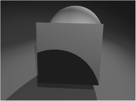
Figure 14-95: Theta
Translucency
Translucency is the quality of a substance’s surface that allows light to diffusely pass through it. As you know, translucency is not the same as transparency. Translucent objects do not reveal the colors or any other attribute of the object that is behind; however, light penetrates the surface and the object behind will show through. The look of translucency is greatly affected by the angle from which the surface is being seen. This node has a Color input where you can connect a texture that will show up in the rendered image at certain angles. The perfect example of this effect is leaves. This shader is almost the same as the Translucency input channel and therefore it works best if it is used alongside another diffuse shader and the two are mixed. A feature that sets this node apart from the channel is that it lets you select the maximum range of light diffusion. In the Node Edit panel you will find a pull-down menu that allows you to select between two Range options: 90 and 180 degrees. This shader works best with thin objects such as paper and window treatments (curtains).
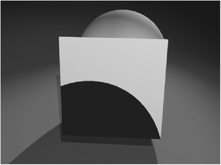
Figure 14-96: Translucency
Reflection Subcategory
Ani-Reflections
Anisotropic reflections are dependent on direction just like anisotropic speculars. Besides being able to connect color attributes to this node, you can also tint the reflection and change the dispersion based on samples. Sampling is the number of directions evaluated in the surface in order to determine its shading value. The more samples, the better the quality, but it comes at a very render-expensive cost. I have found that 3 × 9 or 4 × 12 suits most of my needs most of the time.
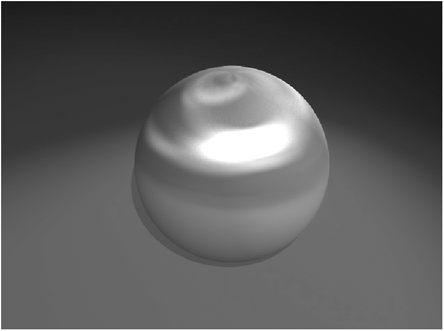
Figure 14-97: Ani-Reflections
Reflections
This is similar to the Reflection slot in the destination node but with some added features. Besides being able to connect color attributes to this node, you can also blur the reflection and change the dispersion based on samples. Sampling is the number of directions evaluated in the surface in order to determine its shading value. The more samples, the better the quality, but it comes at a very costly render expense. You can tint the reflections as well.
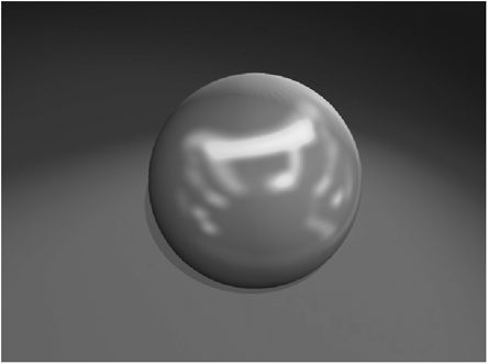
Figure 14-98: Reflections
Specular Subcategory
Anisotropic
Anisotropic speculars are dependent on direction. This is a great model to use with materials (usually man-made) that have tiny grooves in them such as brushed metal, stainless steel, and the classic example… CDs. The Anisotropic specular shader will also do a great job with fibrous objects like Christmas ball ornaments and velvet. In the Node Edit panel you will see options that allow you to control the shape and direction of the anisotropic highlight. Anisotropy U and Anisotropy V control the amount of anisotropy, while Axis controls the direction of the highlight. The Mapping pull-down menu gives you three options for the anisotropic shape: Cylindrical, Linear, and UV. You can also offset the position by entering values in the center tab or by connecting a node attribute to the input. Remember that just like every other attribute in the Node Editor, any manually entered values will be overridden once a node attribute is plugged into the input.

Figure 14-99: Anisotropic specular
Blinn
Blinn is the default specular shading model; it simulates the direct reflection of light by a surface, creating a smooth hot spot called a “specular highlight.” Blinn and Phong are almost identical, with the main difference that Phong’s highlight spreads out more. Blinn is computationally more expensive than Phong since the specular highlight tends to be more realistic than Phong. Blinn is great for materials such as glass, shiny metals, plastic, and wet, slimy surfaces.
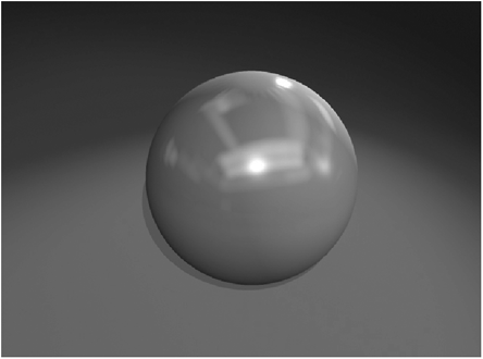
Figure 14-100: Blinn
CookTorrance
This shader model is the most realistic of the specular shaders and is far more versatile. At high glossiness settings, the highlight will get tight and sharp, making it perfect for glossy, reflective materials such as plastic, glass, and water. At lower glossiness settings, the highlight will spread out and diffuse more, as seen on materials with less reflective properties such as skin.

Figure 14-101: CookTorrance
Phong
This specular shading model was developed by Phong Bui Tong in the ’70s. It is computationally faster than Blinn but not as accurate. As mentioned in the Blinn section, the Phong specular highlight spreads out more to the point of causing rims if the light is directly behind the object. Blinn’s specular highlight will remain concentrated and will not spread out like Phong.
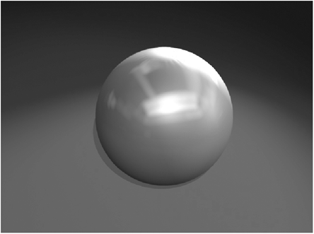
Figure 14-102: Phong
Subsurface Scattering Subcategory
Subsurface scattering (SSS for short) is the phenomenon where light penetrates a semitranslucent surface, scatters inside the volume, and exits at a different angle. SSS is important to accurately represent materials such as milk, wax, and skin, to name a few. LightWave has two shaders to aid you with the creation of such effects: Kappa and Omega. While these are diffuse shaders and can be connected directly to the Diffuse Shading slot in the destination node, you will get better results if you mix the shader with another diffuse shader such as Oren Nayar. SSS is considered by many, including me, to be an advanced technique that requires a bit of experience with the Node Editor and its nodes, as well as good general surfacing skills. That said, I still wanted to cover these shaders here just in case you feel adventurous. The reality of SSS is that there is no right “recipe” to get good effects in your models, but there are some things you can think of when trying it:
• The physical size of the object
• The apparent thickness of the object
• The lighting environment
• The type of material
• The object’s internal volume
SSS is found in different type of materials and is different in all of them. Wax and skin are good examples. Wax, while a solid surface, has no internal structures (besides the wick) so light has more room to scatter before it exits. Skin has a more complex structure; we have muscles, veins, organs, bones, etc., and light will interact with all of these elements before it exits and therefore the SSS effect will be different.
Kappa
Kappa is also known as a “fake SSS” effect. It is not based on an accurate SSS model but its advantage is that it is a lot faster than a physical model like Omega. Like Omega, Kappa works best in a ray-traced environment, so make sure you turn ray tracing on in the Render Globals panel. If you open the Kappa Node Edit panel, you will see the following options:
Color — Determines the color of the surface; you can enter an RGB value manually or you can connect attributes from other nodes in the network.
Range — Essentially determines how deep inside the volume you would like the samples to reach. This is why you need to have in mind the actual size of your object. A 1m object with a 10mm range will look different from a 0.5m object with a 10mm range. Using the same wax and skin examples, wax will have a greater range than skin.
Amount — This is the intensity of the SSS effect, or how strong it is.
Samples — Determines the number of directions a surface evaluates in order to calculate the SSS solution, so the higher the number, the better the quality and therefore the longer it will take to render. I tend to use 2 × 6 for test renders and 4 × 12 for final renders. If it is not enough, I’ll go to the next option down the list.
Mode — Here you select between Forward, which means that the main light source is coming from a similar direction as the viewer, and Backward. Backward means that the light source is away from the viewer, like in backlit environments.
Of course, lighting changes from scene to scene depending on the mood that you are trying to convey, but in most cases you should use a mix of two Kappa nodes, one set to Forward and the other set to Backward. This will give you good results in most lighting situations.

Figure 14-103: Kappa
Kappa II
In Kappa (described above) you can select either forward or backward scattering, making it necessary to build a two-Kappa node network to create a convincing SSS effect in your surface. Kappa II streamlines this process by providing the ability for you to select forward and backward colors and amounts in a single node. There are no other “extra” options in this node; it simply combines two Kappa nodes into one.
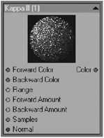
Figure 14-104: Kappa II
Omega
Omega is NewTek’s implementation of a physically correct SSS shading model. We all know what “physically correct” means… long render times! Omega has some options to help reduce render times a bit, though. In order to create a good SSS surface with this shading model, you need to have either an “air” surface, which is a duplicate object with the poly normals flipped so that they face inward, or you can use the Spot Info node along with a Logic node in order to give each side of the polygons a different refraction index. This is the method I use since “air” polys can produce artifacts in the render. If you are new to subsurface scattering, start with Kappa; Omega is more challenging so it’s better to start easy and then expand on it once you feel comfortable enough. Let’s review the options in this node’s Edit panel.
Surface Color — Determines the color of the surface; you can enter an RGB value manually or you can connect attributes from other nodes in the network.
Subsurface Color — Determines the color of the subsurface; you can enter an RGB value manually or you can connect attributes from other nodes in the network.
Color Falloff — Determines at what percentage of penetration the subsurface color is at 100%.
Falloff Bias — This is a curve that will favor color falloff over surface color (start) or subsurface color (end).
Amount — This is the intensity, or how strong the SSS effect is.
Spread — Determines the variation amount of the evaluation ray’s distribution over a surface. High values mean wider angles, while smaller values mean tighter angles.
Index of Refraction — Determines how much light bends while traveling through the material.
Penetration — Determines the distance at which the subsurface color is at 100% falloff. This is affected by both Color Falloff and Falloff Bias.
Mode — Here you select the method of evaluation for the surface.
• Single Scattering (No RayTracing) — All of the options that use No RayTracing calculate thickness by firing a “measurement” ray, so other properties in the scene like Ray Trace Reflections are not calculated.
• Single Scattering (Full RayTracing) — Full RayTracing allows other objects and properties in the scene environment to be taken into account during the evaluation, which in turn affects the look of the SSS effect.
• Multiple Scattering (No RayTracing) — This works the same as Single Scattering but the ray bounces inside of the surface multiple times, collecting samples before it exits.
• Multiple Scattering (Full RayTracing) — Try this setting if you feel courageous. It works the same as the option above, but it takes into account ray tracing of the scene environment and objects and is therefore the most computationally expensive option of the bunch.
Samples — Determines the number of directions a surface evaluates in order to calculate the SSS solution, so the higher the number, the better the quality and therefore the longer it will take to render. I tend to use 2 × 6 for test renders and 4 × 12 for final renders. If that is not enough, I’ll go to the next option down the list.
Recursions — This is the value used by the Multiple Scattering options described above.
By selecting one of the No RayTracing options you can save a lot of render time. It is still slower than Kappa but it is better than using Full RayTracing.

Figure 14-105: Omega
Transparency Subcategory
The shaders in this section are intended to be connected to the Refraction Shading slot of the surface destination node. These nodes work in direct correlation with the Basic Transparency value of the Surface Editor or the Transparency attribute in the surface destination node. By applying a different set of normals you can achieve the illusion of depth in a layered surface, like carbon fiber, for example.
Ani-Refractions
This shader allows for anisotropic qualities to the refraction of a transparent surface, like quartz or ice, for example. The top section of the Node Edit panel is very similar to that found in the Refraction Options in Surface Editor’s Environment tab, where you can select from a list of refraction mapping modes and an image to refract. In this node you have the option to tint the refractions, and the color can be animated. Another useful option is Dispersion, which is the phenomenon where a wave is divided into components with different Index of Refraction (IOR) levels. The perfect example of this would be a prism.
Refractions
This is another refraction shader that provides you with more control over the refraction look of the surface. As in Ani-Refractions, you can tint the refraction and you can add dispersion as well. Here you also have the option to blur the refraction; the quality of the blurring is derived from the Samples option that you select. Just keep in mind that with high sampling levels, the render times will take a serious hit. Find a good balance between quality and speed.

Figure 14-106: Tinted Refraction
Spot
The only node in this category is Spot Info. Spot Info gives you access to data regarding the current spot. Let’s translate that into something a little more understandable. A spot is a pinpoint of undetermined size being evaluated on the current surface. Since we are working on the Surface Node Editor, the evaluated data corresponds to an object’s surface, such as the length of the incoming ray, its source, and where it is headed relative to the spot being evaluated. There are many uses for this node, ranging from normal and displacement maps to creating double-sided surfaces with different properties on each side of the polygon. Since Spot Info simply evaluates the surface and returns information, there are no inputs available; however, the information is available as outputs that you can connect to other nodes in the network. The Spot Info outputs and their types are as follows:
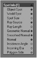
Figure 14-107: Spot Info node
Object Spot (vector) — This is the current spot being evaluated in Object Coordinates XYZ.
World Spot (vector) — This is the current spot being evaluated in World Coordinates XYZ.
Spot Size (scalar) — The size of the spot being evaluated.
Ray Source (vector) — The XYZ position of the ray source.
Ray Length (scalar) — This outputs the length of the ray from the ray source to the spot being evaluated.
Geometric Normal (vector) — Determines the normal information of the flat-shaded polygon being evaluated by the current spot.
Smoothed Normal (vector) — Determines the normal information of the smooth-shaded polygon being evaluated by the current spot.
Normal (vector) — Determines the normal information of the smooth-shaded, bump-mapped polygon being evaluated by the current spot.
Incidence Angle (scalar) — This is the incidence angle between the source ray and the normal.
Incoming Eta (scalar) — This is the incoming refraction index.
Polygon Side (integer) — This determines the sides of a double-sided surface. The back side is 0 and the front side is 1.
Tools
This category contains tools to help you with different tasks while building nodal networks. They allow you to make “type” conversions and mix nodes together using different modes.
Color Scalar
This node is used to convert a Color output to a Scalar output. In the Node Edit panel you have a pull-down menu where you can select a method of conversion. They are as follows:
Figure 14-108: Color Scalar node
Average — Outputs the scalar value by averaging the values of the color RGB components. Scalar = (R+G+B)/3.
Maximum — The Scalar output takes the largest value of the three RGB values.
Minimum — The Scalar output is the smallest value of the three RGB values.
Red Channel — Outputs the scalar value by using the Color input’s red channel value.
Green Channel — Outputs the scalar value by using the Color input’s green channel value.
Blue Channel — Outputs the scalar value by using the Color input’s blue channel value.
Luma — The scalar outputs the luminance value from the Color input.
Color Tool
The Color Tool lets you adjust several color properties in a single node based on the HSV color model. Most likely you have used this in an image editor such as Photoshop before, but here is a quick rundown of the available options.
Color — This is the color that will be affected by the other attributes of the node. It can be an incoming color from other nodes in the network, or manually specified.
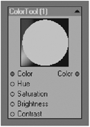
Figure 14-109: ColorTool
Hue (H) — Measured as degrees from 0 to 360 on the standard color wheel. You can change the hue of the input color by changing the degree value, essentially going around the color wheel.
Saturation (S) — Determines how much of the hue you see. The default of 100% means that the input color remains the same, while a value of 0% means that the hue is completely gone, leaving you with a grayscale image. Any values over 100% will accentuate the hue further.
Brightness (V) — Determines how light or dark the color is. As with Saturation, this is measured with a percentage value. The default value of 100% means no change in brightness, and a value of 0% means black. A value over 100% will incrementally be changing to white.
Contrast — Controls the tonal range of an image. The colors of a low-contrast image will look dull, which makes it hard to differentiate between foreground and background elements. On the other hand, an image with high-contrast values will have richer colors and elements will be easier to see. An image with too much contrast will look almost neon-like and the image will have a posterized look.
Limiter
Limiter is basically a clamp that works on every channel of the Color input RGB channels at once. The RGB will not go above or below the specified Low and High input values.
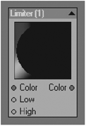
Figure 14-110: Limiter
Make Color
This node allows you to create a Color output based on Scalar inputs, either manually entered in the Node Edit panel or by connecting attributes from other nodes in the network.
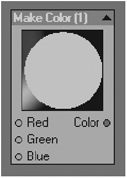
Figure 14-111: Make Color
Make Vector
This node allows you to create a Vector output based on Scalar inputs, either manually entered in the Node Edit panel or by connecting attributes from other nodes in the network.

Figure 14-112: Make Vector
Mixer
You will be using this one quite often. It allows you to mix between two color type inputs based on the blending modes that I talked about earlier in this chapter. This is a great node for mixing any color inputs, including shaders!
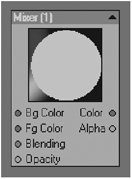
Figure 14-113: Mixer tool
Vector Scalar
This node is used to convert a Color output to a Scalar output. In the Node Edit panel you have a pull-down menu where you can select a method of conversion. They are as follows:
Maximum — The Scalar output takes the largest value of the three vector components (XYZ).
Minimum — The Scalar output takes the smallest value of the three vector components (XYZ).
X Channel — Outputs the scalar value by using the Vector input X channel value.

Figure 14-114: Vector Scalar node
Y Channel — Outputs the scalar value by using the Vector input Y channel value.
Z Channel — Outputs the scalar value by using the Vector input Z channel value.
Length — Outputs the scalar value by using the Vector input length.
Vertex Map
These nodes allow you to access the information of vertex maps that were created in Modeler.
Morph Map
This node gives you access to any morph map that you have created in Modeler. With this node and a little logic we can change the color of an object based on the amount of morph being applied to it.

Figure 14-115: Morph map
Vertex Map
This node gives you access to any vertex color maps available in your object. You have the ability to mix the vertex map with other color nodes in the network. You can then connect the Color output to different nodes’ attributes or simply connect it to the Color input of the destination node.

Figure 14-116: Vertex map in action
NOTE: See Chapter 7 for more on the creation of color vertex maps.
Weight Map
This node gives you access to every weight map available in your object. You select the map in the Node Edit panel’s pull-down menu. The Value output can be connected as-is to other node attributes, but to gain more control you can connect the value output to a gradient’s input; this way you can control the map using the values of a gradient.
NOTE: Check out the Canyon tutorial in Chapter 24 on to see weight maps in a real-world example.
Putting Nodes to Work
Now that we have gone through all of the different nodes available in the Node Editor and have a better understanding of the job they perform, it’s time to put them to work with some quick exercises. I admit that some of those nodes might not make a heck of a lot of sense right now, but after these exercises, things will begin to “click.”
Blending Images with Gradients
In the “Gradient” section I told you that you can use the key outputs of a gradient to blend images together; here is how to go about doing that.
1. Load up the scene called blending_images.lws from TutorialsNode Editor on the companion CD. As you can see, it is a simple sphere.
2. Open the Surface Editor (F5) and select the “sphere” surface from the Surface list, then click on the Edit Nodes button to open the Node Editor. To better see what we are doing, open VIPER (F7) and make a render to save the buffers for VIPER.
3. Add a couple of image nodes to the workspace by going to the Add Node pull-down menu or by accessing the contextual menu by pressing Ctrl+ right mouse button, and then choosing Add Node>2D Texture>Image.
4. Now with the image node selected, double-click it to open its Edit panel. If you have the Edit panel embedded to the Node Editor, the panel should show just by clicking on the node. Load the image called newtek_concrete16.jpg, set MipMap Quality to Off and Mapping to Spherical, and then click on the Automatic Sizing button to fit the texture to the sphere’s size. With one image node set up, you can copy (Ctrl+c) and paste (Ctrl+v) the node, so now the only thing you need to change is the actual image to be used. Open the Node Edit panel of this node and load a different image; you can load stone06.jpg.
5. With the image nodes ready, we can now set up the gradient. Add a gradient node to the workspace by choosing Add Node>Gradient> Gradient. Connect the Color output of the gradient node to the Color channel of the surface destination node.
6. Double-click on the node to open the Edit panel. All we need to do now is add an extra key to the gradient and change the key color to white. This is not absolutely necessary to do, but it will give you a better idea of how the blending is being controlled by the gradient.
7. Before we make any connections, change the input of the gradient to Y Coordinate. Now that we are ready to make connections, activate Show Output for both keys in the gradient. Six more connections are added to the list of the node, three for each key on the gradient; they correspond to Color, Position, and Alpha.
8. Connect the Color output of Image 2 to Key (1) color. Once you do this VIPER should update. It’ll be a little too grainy, so make a render to better see the result. You should see a white sphere (Key 2 color) and the texture of Image 2, which is a little faint but it is there. At this point you can fine-tune the keys of the gradient to adjust the blending if desired.
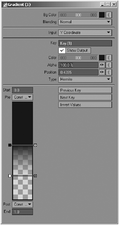
Figure 14-117: Gradient with keys adjusted
9. Connect the Color output of Image 1 to Key (2) color; VIPER should update again and now you can clearly see that the color of Key 2 has been replaced with the image. You can fine-tune the gradient’s keys to suit. You can also keep adding as many keys and images as you want, memory dependent, of course. Before, in the “classic” Texture Editor, you had to create an alpha gradient layer for each image on the stack, which made it a tedious task to edit them. Now you have just one gradient node doing all the blending for you, which is much easier to edit.

Figure 14-118: Two images blending
I took this a little further; I added a Crumple 3D texture and connected it to the Bg Color of the gradient node. Then I changed the Alpha of Key 2 on the gradient to 50%. The result is that the image is 50% transparent, therefore allowing the Bg Color to show through. I also added an Add vector node and connected the Bump output of both images to the inputs A and B. The result output is then connected to the Bump channel of the surface destination node. I finished this surface off by adding a Divide node and connecting the Image1 Luma output to the A input of the Divide node. The B input is 0.8, which I entered manually in the Node Edit panel. The result output was connected to the Diffuse, Specular, and Glossiness channels of the surface destination node. If you feel that the surface is too bumpy, you can reduce the Bump Amplitude attribute of the image nodes. You can see this network in Figure 14-120; this is also available as a preset named LW9T_imgBlend on the companion CD.
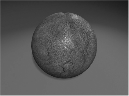
Figure 14-119: The final surface
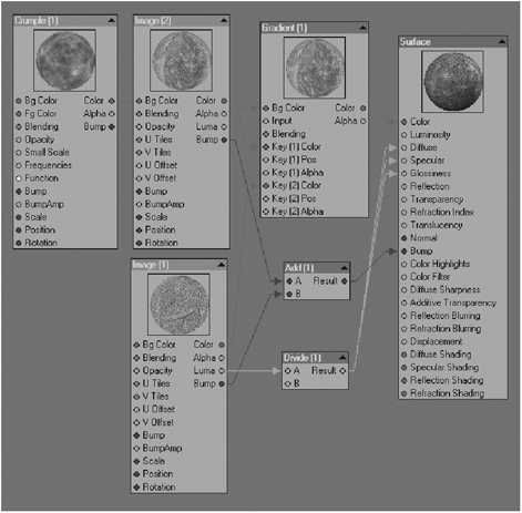
Figure 14-120: The finished node network
TIP: Visit the NewTek web site to register and gain access to a great texture collection. The images used here are samples from this collection.
Assigning Different Textures to Double-sided Surfaces
Before LightWave v9 if you wanted to make very thin objects with different textures on each side of the polygons, such as book pages, you would have to make a copy of the polygons, flip them, and offset them a tiny bit so they are no longer on top of each other and to avoid Z sorting problems.
LightWave v9 has a node in the Node Editor that can differentiate one side of the polygon from the other, allowing you to do several different things previously tough or inefficient to do in the “classic” Texture Editor. This node is called Spot Info (Add Node>Spot>Spot Info). This node has an attribute at the bottom of the list called Polygon Side. This attribute’s type is integer, outputting 0 (black) for the back side or 1 (white) for the front side.
We can use this information in a number of different ways; for this exercise we are going to assign different textures to each polygon side.
1. To do this we can use the handy Mixer node (Add Node>Tools>Mixer); change the Bg Color to a very light beige color, which will be the inside of the apple; then change the Fg Color to a green color, which will be the skin of the apple.
2. Connect the Color output of the Mixer node to the Color channel of the surface destination node. Now make a test render to see what we have so far and to save the buffers for VIPER.
You will notice that the apple peel object is the same color on both sides (Figure 14-121); that’s because we haven’t connected the Polygon Side output of the Spot Info node.
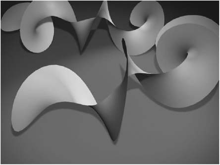
Figure 14-121
3. Just connect that output to the Opacity input of the Mixer node and make another test render. Now you should see each side of the polygons with the colors we assigned in the Mixer node, as seen in Figure 14-122.

Figure 14-122
All we have left to do is make it look more like an apple peel with some textures.
4. I added a Crumple (Add Node>3DTextures>Crumple) and an Image (Add Node>2DTextures>Image) node. For the crumple texture I increased its size quite a bit: Scale X 10m, Y 5m, Z 10m; this makes the crumple texture really large and gives us the hint of the surface on the other side. I also made the background color a light beige color and the foreground color the same apple green as seen on the tiling 2D apple texture found on the companion CD.
5. I loaded this apple tiling texture to the Image node, changed UV Tiling to 2, and Planar mapped on the x-axis of the object.
Now we have an object with different textures on both sides of a double-sided object without the need of duplicate polygons and two separate sets of surfaces. You can take this further by adding a clip map to add irregularities on the border edges.

Figure 14-123: Apple peels
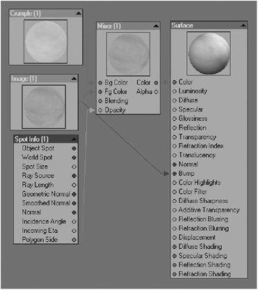
Figure 14-124: The apple peel’s node network
Let’s take a look at another Polygon Side example.
Air Polys No More!
Prior to LightWave v9, in order to create realistic glass you needed a duplicate copy of your glass object with the polygon normals flipped, then you had to assign an IOR (Index of Refraction) of 1 and a very high transparency value to correctly duplicate how light rays enter a surface and bend and exit on the other side. This is called an air polygon. This approach has two major drawbacks: One, it increases the poly count of the object and two, you have two different surfaces to deal with.
With the help of the Spot Info and Logic nodes in LightWave v9, we can assign different IORs to both sides of the polygons and thus get rid of duplicate geometry while accurately replicating the effect of air polys.
NOTE: Refer to the previous sections of this chapter for a description of these nodes.
1. Load the scene called spot_info_glass.lws from the companion CD if it isn’t already loaded. Make sure that Double Sided is on for the sphere surface in the Surface Editor; also make sure Ray Tracing is on in the Render Globals panel.
2. Open the Node Editor like we have done before, and then add a Spot Info node (Add Node>Spot>Spot Info) and a Logic node (Add Node>Math>Scalar>Logic).
3. Connect the Polygon Side output of the Spot Info node to the A input of the Logic node.
4. Go to the Logic node Edit panel and change the If True attribute to something other than 1 (let’s try 1.1 for now).
5. Now, connect the output of this node to the Refraction Index channel in the surface destination node.
We know that the front side of the double-sided poly is identified as 1 and the back side as 0, so basically what the Logic node is saying is, “If A(1) equals B(0), then the statement is True and therefore 1.1 will be the value used for the refraction index. If A(1) doesn’t equal B(0), then the value used as the refraction index will be 1.0.”
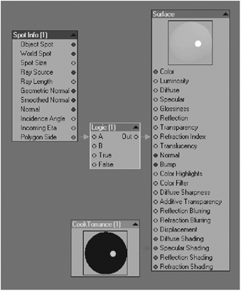
Figure 14-125: Glass node network
Before making a test render, assign a transparency amount to the sphere surface se we can actually see the refraction at work. Also go ahead and load the “dirty floor” surface preset for the plane surface so there is something for the sphere to refract; this preset is found on the companion CD. Now make a test render to see your results. Play with the refraction values to see the effect. Cool, right? Adios, air polys!
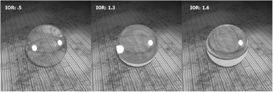
Figure 14-126: Different IOR for the sphere
Making Targeted Eyes
At one point or another we probably have all made eyes with a simple gradient, whether they were realistic or cartoony. If not, then these will be your first! As you can probably imagine, eyes can be created easily with a gradient set with multiple colors. That’s the easy part. But how do you make the gradient target an item in the scene using the Node Editor? Ah, now things get a bit more complicated. Don’t worry, though, it really isn’t all that tough.
1. Load the scene called eye_follower.lws. This scene is quite simple; just a sphere, aka the eyeball, a camera, and a couple of lights.
2. Open the Surface Editor and then open the Node Editor by clicking on the Edit Nodes button.
3. Create a Gradient node (Add Node>Gradient>Gradient), then create the color keys for your eye. Figure 14-127 shows the gradient I created. Most likely you used Incidence Angle as the input parameter, but for the eye to properly target the null, use Z Coordinate instead. The gradient will look slightly different as it isn’t using the camera viewing angle anymore.
4. Now create a null object and place it in front of the eye.
5. Select the eyeball object and open the Motion Options panel (m). Click on the Target Item pull-down menu and select the eye-ref object.
That’s it! Move the null object around and make test renders to see the eyeball correctly targeting the null.

Figure 14-127: Gradient

Figure 14-128: Targeted eye
NOTE: VIPER cannot preview this setup properly. To assure it works, you need to make test renders (F9).
Skin with Subsurface Scattering (SSS)
As technology and computer power have evolved, so have the techniques used to achieve realism in our work. Subsurface scattering is an example of this. SSS has become very popular in the last few years and now we have two built-in shading models to help us with this effect. I consider SSS to be an advanced technique best explored when you have a full understanding of texturing, building node networks, and lighting, but if you feel adventurous, by all means experiment with it. In this exercise we are going to build two nodal networks. The first one is based solely on Kappa, which renders more quickly than Omega. The second network that we are going to create is based on a mix of the SSS models Kappa and Omega, but be warned; since it uses Omega, it is far slower than an exclusive Kappa setup. This technique was developed by fellow artist Werner Ziemerink, who also provided the awesome Scientist model and maps for us to work with.
Kappa SSS
1. Load up the scene called SSS_Scientist.lws, then open the Surface Editor and select the Head surface from the list.
2. Open the Node Editor and start by adding an Image node (Add Node>2D Textures>Image). Now open its Edit panel and load the image called M_Head_bump.jpg, switch MipMap Quality to Off, and set the projection to UV.
3. Select the OBJ_texture UV map from the pull-down menu and set Bump Amplitude to 32%. Connect the node’s Bump output to the Bump input of the surface destination node.
4. Since we have an image node set up, copy and paste it on the workspace. Open its Edit panel and load the image called M_Head_spec.jpg, then add a Blinn node to the workspace (Add Node>Shaders>Specular>Blinn). Connect the spec image node’s Luma output to the Specular input of the Blinn node, change the Blinn’s Glossiness setting to 40%, then connect the Color output of the Blinn to the Specular Shading slot of the surface destination node.
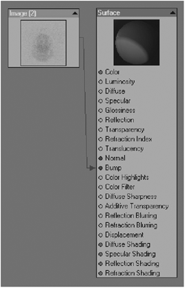
Figure 14-129: Bump
5. Add a Kappa node to the workspace (Add Node>Shaders>Subsurface Scattering>Kappa). Also paste the image node again (it should still be stored in the clipboard), open its Edit panel, and load the image called skin2.png. Connect the Color output of the image node to the Color input of the Kappa node. In the Kappa Edit panel, enter 25mm as the Range and set Amount to 100%. I generally use 2 × 6 samples for test renders and 3 × 9 or 4 × 12 for final images; this is up to you, but remember that the higher the sample number, the longer the render times will be as well. Make sure the Kappa mode is set to Backward. In order to have a nice SSS effect for characters using Kappa, we need two Kappa nodes, one for the back (backscatter) and one for the front (epidermis). NewTek developed another SSS node called Kappa II, which combines this two-Kappa node setup into one single node and therefore streamlines the process. Figure 14-130 shows the network so far.

Figure 14-130
6. Paste the image node once more, then open its Edit panel and load the image called skin.png, and set Blending Mode to Multiply. Now copy and paste the Kappa node, change Range to 12mm, Amount to 90%, and Mode to Forward. Connect the Color output of the image node to the Color input of the Kappa node we just created. If you right-click on this Kappa node or hit “r” on your keyboard, you can rename it to something a little more descriptive, like “Kappa-forward.”
7. I wanted to saturate the image color a little, and there are a few ways to do this. In this case we can just use a color node (Add Node>Constant> Color), make this an orange-reddish color, and connect the Color output to the Color input of the skin image node. This will saturate the image a little since Blending Mode is set to Multiply. Figure 14-131 shows the Kappa network.

Figure 14-131: The Kappa network
8. In LightWave v9, as you know by now, we can change the Diffuse shading model to something other than the default Lambert. Let’s add an OrenNayar node to the workspace (Add Node>Shaders>Diffuse> OrenNayar).
9. Connect the Color output of the skin image node to the Color input of the OrenNayar node. Open its Edit panel, and change the Diffuse value to 60% and Roughness to 35%.
10. All we have left to do is connect all of these diffuse shaders together; to do this we can use our handy Mixer tool (Add Node>Tools>Mixer). First we are going to connect the Kappa nodes together by connecting the Color output of Kappa-backward to the Bg Color input of the Mixer node, and connecting the Kappa-forward Color output to the Fg Color input of the mixer node. Next we want to connect the OrenNayar node to the rest of the network. To do this, copy and paste another Mixer node in the workspace. Connect the Color output of Mixer (1) to the Bg Color of Mixer (2), and the Color output of OrenNayar to the Fg Color of Mixer (2). Finally connect the Color output of Mixer (2) to the Diffuse Shading slot in the surface destination node. Figure 14-132 shows the finished node network.
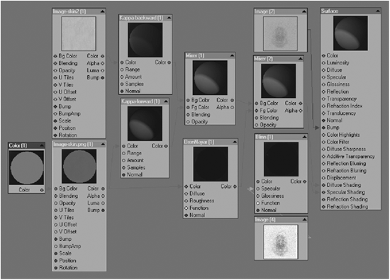
Figure 14-132: Finished node network
11. You can now make test renders since VIPER doesn’t gives an accurate representation of the SSS effect. If you feel that it might be too waxy looking, then play with the number of variables in the nodal network. Play with the Kappa amounts and ranges as well as the colors and try the different Diffuse and Specular shading models to see what you come up with. Make a preset of this shader for later use. Figure 14-133 shows the final result with a bloom layer created in Photoshop. The bloom layer is simply a copy of the base layer with the colors saturated using levels and then blurred. This layer is then screened over the base layer; play with the opacity to control the amount of bloom.
Omega SSS
Omega yields better results than Kappa, but the drawback is that it is painfully slow. If you have the time and render power, then I think you will be happier with the results of Omega for skin in particular. The following setup uses a mix of Omega and Kappa.
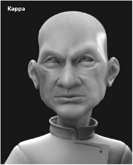
Figure 14-133: The test render
1. Load up the scene called SSS_Scientist.lws. Open the Surface Editor and select the Head surface from the list. Open the Node editor, and add an image node like we did in the Kappa example (Add Node>2D Textures>Image).
2. Load the image called M_Head_bump.jpg, change the Mapping to UV, and select the OBJ_UVTextureMap from the pull-down list. Copy and paste this node a couple of times and load the skin2.png texture to one and the M_Head_spec.jpg texture to the other. Remember that you can change these node names to something more descriptive. I used Bump, Specular, and Color, respectively.
3. Go ahead and connect the Bump map to the Bump slot in the surface destination node.
4. Let’s add a Blinn specular shader to the network (Add Node> Shaders>Specular>Blinn). Connect the Luma output of the Specular texture map to the Specular input of the Blinn shader, and change the Glossiness setting to 25%. Then connect the Color output of the Blinn node to the Specular Shading slot of the surface destination node.
Figure 14-134 shows the nodal network so far.
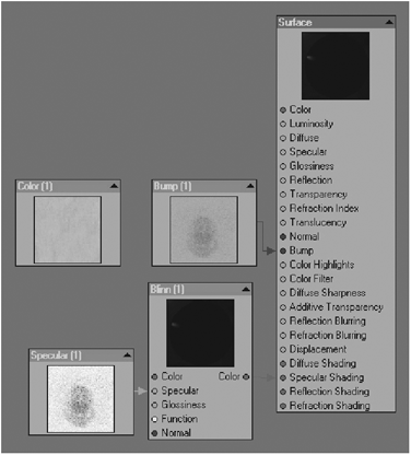
Figure 14-134
5. Let’s add the rest of the nodes needed in the network. We need Kappa and Omega nodes (Add Node>Shaders>Diffuse>Kappa and Omega). We also need a Diffuse shader, so use Lambert this time around (Add Node>Shaders>Diffuse>Lambert), and lastly add a Mixer node (Add Node>Tools>Mixer). Change Blending to Additive and Opacity to 100%. Copy and paste this Mixer tool and put it aside for now.
6. Select the Omega node, and change the settings as follows:
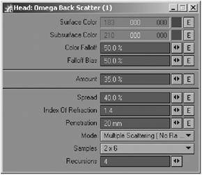
Figure 14-135: Omega
Surface Color: 183, 000, 000
Subsurface Color: 210, 000, 000
Color Falloff: 50%
Falloff Bias: 50%
Amount: 35%
Spread 40%
Index Of Refraction: 1.4
Penetration: 20mm
Mode: Multiple Scattering (No RayTracing)
Samples: 2 × 6 (for testing)
Recursions: 4
7. Select the Kappa node and change the following:

Figure 14-136: Kappa
Color: 247, 165, 111
Range: 12mm
Amount: 75%
Samples: 2 × 6 (for testing)
Mode: Backward
8. With the nodes set up, we can make all of the connections. Connect the Color output of the Omega node to the Bg Color of the first Mixer tool, then connect the Color output of Kappa to the Fg Color of the same Mixer tool. The second Mixer tool is to connect the result of the first Mixer tool and the Lambert shader. Connect the Color output of Lambert to Bg Color of Mixer 2, and the Color output of Mixer 1 to Fg Color of Mixer 2. To finish the setup, connect the Color output of Mixer 2 to the Diffuse Shading slot of the surface destination node. Figure 14-137 shows the finished nodal network, and Figure 14-138 shows the finished image after adding a bloom layer done in Photoshop.

Figure 14-137
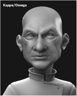
Figure 14-138
Remember that these are just a couple of the many different setups and looks that you can create with SSS. You can use SSS for other semi-translucent materials like milk, candles, plastic, ice, etc.
In Part 7, “Tutorials,” you will find a couple more node-specific tutorials for you to practice with. In Chapter 24 I guide you through the texturing process of a canyon similar to the Grand Canyon or Bryce Canyon using only procedural textures. I also guide you through the making of an ocean. They are both fun and good exercises for creating node networks in both the Surface Node Editor and the Displacements Maps Node Editor.