![]()
Programming even the simplest physics inevitably involves some math. Therefore, we assume that readers of this book are comfortable with math notation and have at least some math knowledge. This knowledge need not be very sophisticated; familiarity with basic algebra and simple algebraic manipulations of equations and formulas is the most important requirement and will be assumed without review. In addition, some appreciation of coordinate geometry and the basics of trigonometry and vectors would provide a good foundation. In case you need it, this chapter provides a review or refresher of these topics. Prior knowledge of calculus is a bonus, but is not essential; similarly for numerical methods. We provide an overview of the basic concepts involved in these topics at a level sufficient to apply them in physics programming.
Topics covered in this chapter include the following:
- Coordinates and simple graphs: Math functions and their graphs crop up constantly in physics applications. We review some common math functions and plot their graphs using a custom JavaScript graph-plotting object. We also show how to make an object move along any curve described by a mathematical equation.
- Basic trigonometry: Trigonometry crops up a lot in graphics and animation in general, and is pretty much an indispensable tool in physics-based animation. In this section, we’ll review some trigonometry essentials that will be used in later chapters. We’ll also get to play with trig functions such as sin and cos to produce some cool animation effects.
- Vectors and vector algebra: Vectors are useful because physics equations can be expressed, manipulated, and coded up more simply using them. After a review of vector concepts, we’ll construct a JavaScript Vector2D object that will be used throughout the rest of the book.
- Simple calculus ideas: Calculus deals with things that change continuously, including motion. It is, therefore, a natural tool to apply to physics. Calculus is usually considered part of advanced math. So we’ll give only an overview of the basic concepts here to show how they can be implemented in physics equations and in code.
Although this chapter consists of review material, much of it covers application of the math in JavaScript and physics. Therefore, even if you have a solid math background, we recommend that you at least skim through this chapter to see how we apply the math.
In our attempt to illustrate the application of otherwise abstract math concepts to physics, we have picked some examples of physics concepts that will be explained more fully in later chapters. So don’t worry if you don’t immediately get everything that we’ll cover here; you can always come back to this chapter as needed.
Coordinates and simple graphs
Coordinate geometry provides a way to visualize relationships expressed as mathematical functions or equations. This section will review some things you’d have covered in your school math classes, but mixed with a lot of JavaScript code to emphasize the application of those math concepts.
To get started, let’s remember how to plot functions on graphs. Say you want to plot the graph of the function y = x2. The first thing you must do is to decide what range of values you want to plot. Suppose you want x to range from –4 to 4. Then what you might have done at school is tabulate the values of x and the corresponding values of y that you get by using y = x2. Then you might have plotted each (x, y) pair of values as a dot on graph paper and then joined the dots to make a smooth curve. Don’t worry; we won’t ask you to do this here. Instead of reaching for graph paper, let’s do it with JavaScript!
Building a plotter: the Graph object
The Graph object is a custom object we created that does just what its name suggests: draw graphs. You’re welcome to have a look at the code, but what it does is quite simple: it has methods that draw a set of axes and major and minor grid lines using the drawing API. It also has a method to plot data. The Graph object takes nine arguments in its constructor:
Graph(context,xmin, xmax, ymin, ymax, x0, y0, xwidth, ywidth)
The first argument is simply the canvas context on which any instance of the Graph object is to be drawn. The next four arguments (xmin, xmax, ymin, ymax) denote the minimum and maximum desired values of x and y. The next two parameters (x0, y0) denote the coordinates of the origin in the canvas coordinate system, in pixels. The final two parameters specify the width and height of the graph object in pixels.
The function drawgrid() takes four numeric arguments, which specify the major and minor divisions:
drawgrid(xmajor, xminor, ymajor, yminor)
It draws corresponding grid lines and labels the values at the relevant major grid locations.
The function drawaxes() takes two optional arguments that specify the text labels on the axes as strings. It draws the axes and labels them, the default labels being "x" and "y".
drawaxes(xlabel, ylabel)
An example will make the usage clear. Suppose we want to plot the function y = x2 over the range of values specified for x from –4 to 4. Then the corresponding range of values of y would be from 0 to 16. This tells us that the graph should accommodate positive and negative values for x, but only needs to have positive values for y. If the available area is 550 by 400 pixels, a good position to place the origin would be at (275, 380). Let’s choose the width and height of the graph to be 450 and 350 so that it fills most of the available space. We will set the range in x and y (xmin, xmax, ymin, and ymax) to be (–4, 4, 0, 20). Sensible choices for (xmajor, xminor, ymajor, and yminor) are (1, 0.2, 5, and 1):
var graph = new Graph(context, -4, 4, 0, 20, 275, 380, 450, 350);
graph.drawgrid(1, 0.2, 5, 1);
graph.drawaxes('x','y'),
You can find the code in graph-example.js, from this book’s download page on http://apress.com. Go on, try it yourself and change the parameters to see the effect. It’s not really hard, and you’ll soon get the hang of it.
Plotting functions using the Graph object
What we’ve done so far is to make the equivalent of a piece of graph paper, with labeled axes on it. To plot a graph, we use the Graph object’s plot() method. This method plots pairs of values of x and y and optionally joins them with a line of specified color:
public function plot(x, y, color, dots, line)
The values of x and y are to be specified as separate arrays in the first two arguments. The third, optional, parameter color is a string that denotes the color of the plot. Its default value is “#0000ff”, representing blue. The last two parameters, dots and line, are optional Boolean parameters. If dots is true (the default), a small circle (radius 1 pixel) is drawn at each point with the specified color. If line is true (the default), the points are joined by a line of the same color. If you look at the code, you’ll see that the dot is drawn using the arc() method, and the line is drawn using the lineTo() method.
Let’s now plot the graph of y = x2:
var xvals = new Array(-4,-3,-2,-1,0,1,2,3,4);
var yvals = new Array(16,9,4,1,0,1,4,9,16);
graph.plot(xvals, yvals);
There’s our graph, but it looks a bit odd and is not a smooth curve at all. The problem is that we don’t have enough points. The lineTo() method joins the points using a straight line, and if the distance between adjacent points is large, the plot does not look good.
We can do better than that by computing the array elements from within the code. Let’s do this:
var xA = new Array();
var yA = new Array();
for (var i=0; i<=100; i++){
     xA[i] = (i-50)*0.08;
     yA[i] = xA[i]*xA[i];
}
graph.plot(xA, yA, “0xff0000”, false, true);
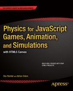
We’ve now used 101 x-y pairs of values instead of just 9. Note that we have subtracted the index i by 50 and multiplied the result by 0.08 to give the same range in x as in the previous array xvals(that is, from –4 to 4). The result is shown in Figure 3-1. As you can see, the plot gives a smooth curve. This particular curve has a shape called a parabola. In the next few sections, we’ll use the Graph class to produce plots for different types of math functions.
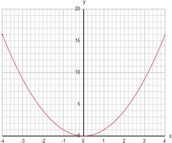
Figure 3-1. Plotting the function y = x2 using the Graph object
We’ll start with linear functions, such as y = 2x + 1. Type the following code or copy it from graph-functions.js:
var canvas = document.getElementById('canvas'),
var context = canvas.getContext('2d'),

var graph = new Graph(context,-4,4,-10,10,275,210,450,350);
graph.drawgrid(1,0.2,5,1);
graph.drawaxes('x','y'),
var xA = new Array();
var yA = new Array();
for (var i=0; i<=100; i++){
     xA[i] = (i-50)*0.08;
     yA[i] = f(xA[i]);
}
graph.plot(xA,yA,'#ff0000',false,true);
function f(x){
     var y;
     y = 2*x + 1;
     return y;
}
Note that we’ve moved the math function to a JavaScript function called f() to make things slightly easier to see and modify.
The graph is a straight line. If you wish, play around with different linear equations of the form y = ax + b, for different values of a and b. You’ll see that they are always straight lines.
Where does the line meet the y-axis? You’ll find that it is always at y = b. That’s because on the y-axis, x = 0. Putting x = 0 in the equation gives y = b. The value b is called the intercept on the y-axis. What is the significance of a? You’ll find out later in this chapter, in the section on calculus.
You’ve already seen that the equation y = x2 gives a parabolic curve. Experiment with graph-functions.js by plotting different quadratic functions of the form y = ax2 + bx + c, for different values of a, b and c, for example:
y = x*x - 2*x - 3;
You may need to change the range of the graph. You’ll find that they are all parabolic. If the value of a is positive, you will always get a bowl-shaped curve; if a is negative, the curve will be hill-shaped.
Linear and quadratic functions are special cases of polynomial functions. In general, a polynomial function is created by adding terms with different powers of x. The highest power of x is called the degree of the polynomial. So a quadratic is a degree 2 polynomial. Higher polynomials have more twists and turns; for example, this polynomial will give you the plot shown in Figure 3-2:
y = -0.5*Math.pow(x,5) + 3*Math.pow(x,3) + x*x - 2*x - 3;
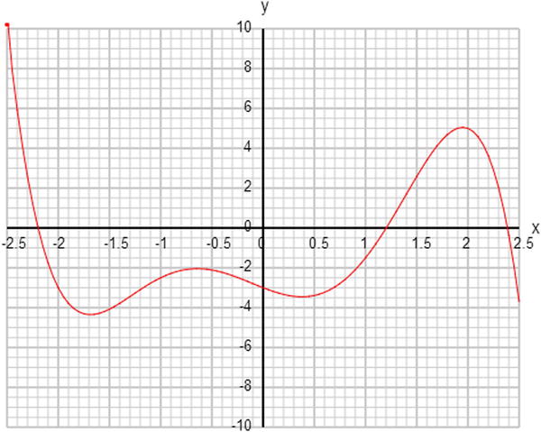
Figure 3-2. A polynomial curve y = –0.5 x5 + 3x3 + x2 – 2x – 3
Things that grow and decay: exponential and log functions
There are many more exotic types of functions that display interesting behavior. One interesting example is the exponential function, which crops up all over physics. It is defined mathematically by
![]()
You might be wondering what e stands for. It’s a special number approximately equal to 2.71828. In this respect, e is a math constant like π, which cannot be written down in exact decimal form, but is approximately equal to 3.14159. Constants such as π and e appear all over physics.
The exponential function is also sometimes written as exp(x). JavaScript has a built in Math.exp() function. It also has a Math.E static constant with the value of 2.718281828459045.
Let’s plot Math.exp(x) then!
As you can see from Figure 3-3, the graph of exp(x) goes to zero as x becomes more negative and increases more rapidly as x becomes more positive. You’ve heard of the term exponential growth. This is it. If you now plot exp(–x), you’ll see the reverse: as x increases from negative to positive values, exp(–x) decays rapidly to zero. This is exponential decay. Note that when x is 0, both exp(x) and exp(–x) are exactly equal to 1. That’s because any number to the power of zero is equal to 1.
Figure 3-3. Exponential growth function exp(x) (solid curve) and decay function exp(–x) (dotted curve)
Nothing stops us from combining functions, of course, and you can get interesting shapes by doing that. For example, try plotting the exponential of –x2:
![]()
This gives a bell-shaped curve (technically it’s called a Gaussian curve), as shown in Figure 3-4. It has a maximum in the middle and falls rapidly toward zero on either side. In Figure 3-4, the curve appears to fall to zero because of the limited resolution of the plotted graph. In reality, it never gets to exactly zero because exp(–x2) becomes vanishingly small for large positive and negative values of x, but never becomes exactly zero.

Figure 3-4. The bell-shaped (Gaussian) function exp(–x2)
Making an object move along a curve
Let’s have some fun and make a ball move along a curve. To do this, we have restructured graph-functions.js and added three new functions to the new code move-curve.js:
function placeBall(){
     ball = new Ball(6,"#0000ff");
     ball.x = xA[0]/xscal+ xorig;
     ball.y = -yA[0]/yscal + yorig;
     ball.draw(context);
}

function setupTimer(){
     idInterval = setInterval(moveBall, 1000/60);
}

function moveBall(){
     ball.x = xA[n]/xscal + xorig;
     ball.y = -yA[n]/yscal + yorig;
     context.clearRect(0, 0, canvas.width, canvas.height);
     ball.draw(context);
     n++;
     if (n==xA.length){
          clearInterval(idInterval);
     }
}
The function placeBall() is called after plotGraph() in init() and simply places a Ball instance at the beginning of the curve. Then setupTimer() is called after placeBall(), and exactly as its name suggests, it sets up a timer, using the setInterval() function. The event handler moveBall() runs at every setInterval() call and moves the ball along the curve, clearing the setInterval() instance when it reaches the end of the curve.
Fun with hills
You can make an object move along the curve of any function you like; for example y = x2. But let’s go crazy and try something more fun, such as this degree 6 polynomial:
y = 0.2*(x+3.6)*(x+2.5)*(x+1)*(x-0.5)*(x-2)*(x-3.5);
You can see that this is a degree 6 polynomial because if you expand out the factors, the term with the highest power of x will be 0.2 x6.
Run the code with this function to see the animation. Does that give you any ideas? Perhaps you could use a curve to represent a hilly landscape and build a game where you try to push a ball over the hills. The only problem is that the curve shoots off to very large values at the ends. This is inevitable with polynomials. The reason is that for large positive or negative values of x, the highest term (in this case, 0.2 x6) will always dominate over the rest. So, in this example, we’ll get very large values because of the effect of the 0.2 x6 term. In the math jargon, the curve “blows up” in those limits.
Let’s remedy this by multiplying the whole thing by a bell function of the type exp(–x2), which, as you know, tends to zero at the ends:
y = (x+3.6)*(x+2.5)*(x+1)*(x-0.5)*(x-2)*(x-3.5)*Math.exp(-x*x/4);
Figure 3-5 shows what we get. Cool. The bell function flattens the curve at the ends, solving our problem. Note that we’ve divided the x2 within the exp() by 4. This is to broaden the bell shape; otherwise, it would kill off the polynomial too quickly, leaving fewer hills. Remove the 4 or replace it with 2 to see what we mean. Try also changing the 4 to 5 or 6 to see the opposite effect.
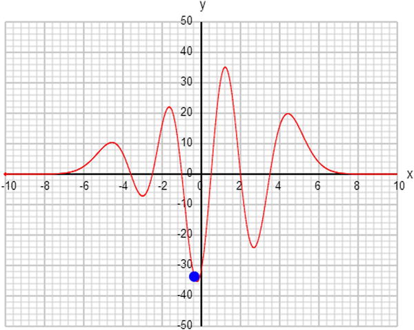
Figure 3-5. Animating a ball on a curve created by multiplying a polynomial and a Gaussian
Here is another way you can modify the curve: multiply it by another factor of x (and an appropriate number to keep it within the range being displayed):
y = 0.5*x*(x+3.6)*(x+2.5)*(x+1)*(x-0.5)*(x-2)*(x-3.5) *Math.exp(-x*x/4);
This modifies the curve in a different way. Because x is small near the origin and large away from it, by multiplying the function by x, we tend to reduce the hills closer to the origin and increase the relative height of the hills farther away. You might notice another change: the value of y for large negative x is now negative, and the landscape starts with a valley instead of a hill because by introducing that extra factor of x, the dominant term in that function is now 0.5 x7. Compare that with the previous 0.2 x6. When the power of the dominant term is odd, it will be negative for negative values of x. But when the power is even, it will be positive even if x is negative. Check this out by multiplying by another factor of x to get this:
y = 0.1*x*x*(x+3.6)*(x+2.5)*(x+1)*(x-0.5)*(x-2)*(x-3.5) *Math.exp(-x*x/4);
If you multiply the function by a negative number, you’ll reverse the whole curve.
There is clearly enormous flexibility in what you can do with functions to create different types of shapes. Hopefully, you might find some use for them! Perhaps build that game that shoots balls over hills. Or maybe get rid of the graph and curve to produce some cool math-based animations without giving away how you’ve done it.
Beyond its use for plotting known functions, the Graph object will come in handy as a useful diagnostic tool to help you visualize what your code is actually calculating, more intuitively and in much greater detail than the humble console.log() function can do. It can help you to understand the logic or physics in your code, and to identify any potential problems. Think of it as a dashboard or instrument panel like the ones in a car or plane, and soon you’ll be using it more than you think!
The trouble with circles
Let’s now try to move an object around a circle using the same method we’ve used in the previous two sections. That should be simple enough, right? First, we need the equation of a circle. You can find this in any elementary geometry textbook.
The equation of a circle of radius r and with origin at (a, b) is given by this:
![]()
If you try to follow exactly the same procedure as in the previous two sections, you’ll want to have y as a function of x. Recalling your algebra, you should be able to manipulate the preceding equation to get this:
![]()
To keep the task simple, choose a = b = 0, and r = 1 (center at the origin, radius of 1):
![]()
Now let’s plot the graph. You’ll want to use the same scaling on both axes so that your circle does not look distorted. If you do just that and run the code, you’ll get something that looks partially correct, but with a couple of strange problems. The first is that you only end up with a semicircle, not the whole circle. The second problem is that the ball takes a little while to appear, and then it disappears at the end. Figure 3-6 shows the resulting plot.
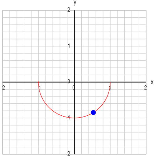
Figure 3-6. First attempt to plot a circle
Let’s deal with the latter problem first. This strange ball behavior arises because we’ve gone outside the range for which the equation makes sense. If you look at the preceding equation, you’ll see that if the magnitude of x is larger than 1, we have the square root of a negative number, which does not give you a real number. So the ball has nowhere to go when that happens!
In contrast to the functions you saw previously, a circle is confined to a limited region of the plane. In math jargon, the function is not defined outside of that range. Let’s fix the code by calculating the value of the function only for values of x in the range –1 <= x <= 1. This is easily done in the loop that calculates the values of the function. Take a look at move-circle.js. This is the modified code that ensures that x is restricted to the correct range:
for (var i=0; i<=1000; i++){
     xA[i] = (i-500)*0.002;
     yA[i] = f(xA[i]);
}
The first problem is trickier. The creation of only a semicircle arises because when we take the square root to get the previous equation, we should have included the negative as well:
![]()
The trouble is that you can’t have a function returning two different values at the same time. There is another problem, this time to do with the animation. You might have noticed that the ball appears to move quickly along some parts of the circle and slowly elsewhere. This isn’t usually what we want to see. It arises because we have been incrementing x in equal amounts. But where the curve is “steep,” the same increment in x leads to a larger increment in y compared with where the curve is more “level.”
Usually we’d want to make an object move in a circle at a uniform rate. Is there a way to know how the position of the ball depends on time and the rate of rotation? There is. It’s time to learn about parametric equations.
The basic problem we had in the last section was that we know y as a function of x, but do not know how either x or y depends on time. What we are after is a pair of equations of this form, where f (t) and g (t) are functions of time:
![]()
![]()
They are called parametric equations because x and y are expressed in terms of another parameter t, which in this instance represents time. From these parametric equations, it should be possible to recover the equation connecting x and y. But the reverse is not necessarily true. Parametric equations are not unique; there might be different pairs of parametric equations that work.
We’ll give you an answer here. Although it won’t make full sense until you’ve done some trigonometry and we’ve covered the concept of angular velocity (in the next section), here it is (where r is the radius of the circle and ω is the so-called angular velocity, which is basically a rate of rotation around the circle):
![]()
![]()
Note that we are using concepts here that will be fully explained only later in this chapter. Therefore, although the concepts might not be completely clear now, they should become so soon enough.
Let’s choose r = 1 and w = 1, and modify the code to compute x and y accordingly (see move-circle-parametric.js):
for (var i=0; i<=1000; i++){
     var t = 0.01*i;
     xA[i] = Math.sin(t);
     yA[i] = Math.cos(t);
}
This does the job perfectly (see Figure 3-7). The multiplicative factor that computes time t from the counter i is chosen to produce at least one complete revolution. Of course, you don’t have to do it this way. You can get rid of the arrays and the loop altogether and just compute x and y on the fly. But it’s good to know that there is another way to animate an object with code apart from computing its position on the fly. This method can prove useful, for example, if the computations are too time-consuming; they could then be done and the positions stored in an array (as done previously) during an “initialization” period, to be animated subsequently in the usual way.
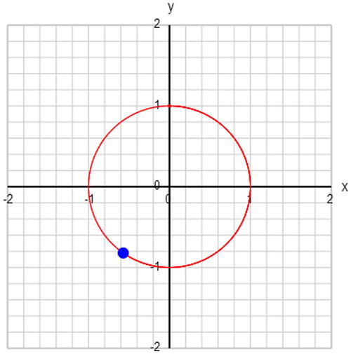
Figure 3-7. Moving an object around a circle using parametric equations
Finding the distance between two points
A common problem is to find the distance between two objects given their locations, which is needed in collision detection, for example. Some physical laws also involve the distance between two objects. For example, Newton’s law of gravitation (covered in Chapter 6) involves the square of the distance between two objects.
Fortunately, there is a simple formula, based upon the Pythagorean Theorem, which allows us to calculate the distance between two points. The Pythagorean Theorem is actually a theorem about the lengths of the sides of triangles. Specifically, it applies to a special type of triangle known as a right triangle, or right-angled triangle, which has one angle that is 90 degrees. The longest side of the triangle, called the hypotenuse, is always opposite the 90-degree angle (see Figure 3-8).
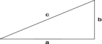
Figure 3-8. A right triangle
The Pythagorean Theorem states that if we take each of the other sides, square their lengths, and add the result, we would get the square of the length of the longest side. Stated as a formula, it is the following, where c is the length of the hypotenuse, and a and b are the lengths of the other two sides:
![]()
Figure 3-9 shows how we use this formula to calculate the distance between two points: by drawing a right triangle. If the coordinates of the two points are (x1, y1) and (x2, y2), the length of the two shorter sides are (x2 – x1) and (y2 – y1), respectively.
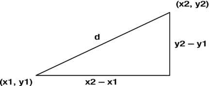
Figure 3-9. Using the Pythagorean Theorem to calculate the distance between two points
Therefore, the length of the hypotenuse, which is actually the distance d between the two points, is given by this:
![]()
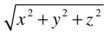
The distance d is then obtained by taking the square root of the previous expression. That’s it. What’s more, this formula can be readily generalized to 3D to give the following:
![]()
Note that it does not matter if we take (x1 – x2)2 instead of (x2 – x1)2, and similarly for the other terms, because the square of a negative number is the same as that of the corresponding positive number.
Trigonometry is a branch of math that technically deals with the properties of triangles and the relationships between the lengths of their sides and their angles. Put this way, trigonometry may not sound very special, but it is, in fact, an indispensable part of your toolset as an animation or game programmer. For example, we used trigonometric functions previously in the parametric equations that produced uniform motion around a circle.
You probably remember the basics from your school days, such as the theorem that the sum of interior angles in a triangle is 180 degrees. But perhaps you may not remember what a sine function is. This section will review the essentials of the subject.
Everyone knows that there are 360 degrees in a complete revolution. Far fewer people know that 360 degrees equal 2π radians (or maybe have never even heard of a radian). So let’s start by explaining what a radian is.
The short explanation is this: a radian is a unit of angular measure (just like a degree is). Here’s how the two measures are related:
- 2π radians is equal to 360 degrees
- so π radians is equal to 180 degrees
- so 1 radian is equal to 180/π degrees, which is approximately 57.3 degrees
Now you might not feel very comfortable with the idea of a radian at all. Why do we need such a weird unit for angle? Don’t we all know and love the degree? Well, the point is that the degree is just as arbitrary—why are there 360 degrees in a circle? Why not 100?
In fact, the radian is in many ways a more “natural” unit of angle. This follows from its definition: the angle subtended at the center of a circle by an arc that is equal in length to its radius. See Figure 3-10.
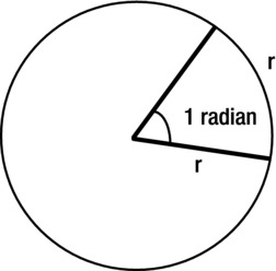
Figure 3-10. A radian is the angle subtended at the center of a circle by an arc of length equal to the circle’s radius
You will frequently need to convert between degrees and radians. So, here is the conversion formula:
- (angle in degrees) = (angle in radians) × 180 / π
- (angle in radians) = (angle in degrees) × π / 180
The trigonometric functions are defined in terms of the sides of a right triangle. Referring to Figure 3-11, you know that the hypotenuse (hyp) is the longest side of the triangle and is opposite the right angle. Pick one of the other angles, say x. Then, in relation to angle x, the far side that does not touch x is called the opposite (opp). The near side that does touch x is called the adjacent (adj). Note that opposite and adjacent are in relation to your chosen angle (x in this case). In relation to the other angle, the roles of opposite and adjacent are reversed. On the other hand, the hypotenuse is always the longest side.

Figure 3-11. Definition of hypotenuse, adjacent, and opposite sides of a right triangle
The sine function is defined simply as the ratio of the length of the opposite side to that of the hypotenuse:
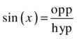
Now you could draw lots of right triangles for different angles x, measure opp and hyp, calculate their ratio, and tabulate and plot sin (x) to see what it is like. But surely you’ll prefer to dig out that Graph object and plot Math.sin(). This is what we’ve done in trig-functions.js.
Figure 3-12 shows what we get. We’ve plotted between –720 degrees (–4π radians) and 720 degrees (4π radians) to show the periodic nature of the function. The period (the interval over which it repeats) is 360 degrees, or 2π radians. The curve is like a smooth wave.
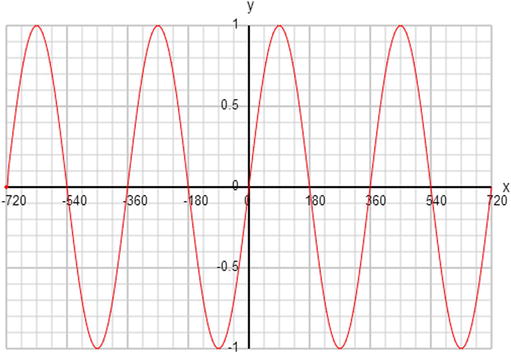
Figure 3-12. The graph of a sine function
Note that sin (x) is always between –1 and 1. It can never be larger than 1 in magnitude, because opp can never be larger than hyp. We say that the peak amplitude of a sine wave is 1. The value of sin (x) is zero at 0 degrees and every 180 degrees thereafter and before.
Similar to sine, the cosine function is defined as the ratio of the length of the adjacent side to that of the hypotenuse:
The graph shown in Figure 3-13 is similar to that of sin (x), except that cos (x) appears to be shifted by 90 degrees with respect to sin (x). In fact, it turns out that cos (x – π/2) = sin (x). Go ahead and prove it by plotting this function. This shows that cos and sin differ only by a constant shift. We say they have a phase difference of 90 degrees.

Figure 3-13. The graph of a cosine function
A third common trig function is the tangent function, defined as follows:
This definition is equivalent to this:
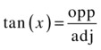
If you plot the graph of tan x, it might look a bit weird at first sight (see Figure 3-14). Ignore the vertical lines at 90 degrees, and so on. They shouldn’t really be there. The graph is still periodic, but it consists of disjointed branches every 180 degrees. Also, tan (x) can take any value, not just a value between –1 and 1. What happens at 90 degrees is that tan (x) becomes infinite. Going back to the definition of tan (x), this is because for 90 degrees, adj is zero, so we end up dividing by zero.
Figure 3-14. The graph of a tangent function
You probably won’t use tan nearly as much as sin and cos. But you will definitely use its inverse, which we’ll introduce next.
It is frequently necessary to find an angle given the value of the sin, cos, or tan of that angle. In math, this is done using the inverse of the trig functions, called arcsin, arccos, and arctan, respectively.
In JavaScript, these functions, which are called Math.asin(), Math.acos(), and Math.atan(), take a number as argument. Obviously, the number must be between –1 and 1 for Math.asin() and Math.acos(), but can be any value for Math.atan().
Note that the inverse trig functions return an angle in radians, so you have to convert to degrees if that’s what you need.
There is another inverse tan function in JavaScript: Math.atan2(). What is the difference, and why do we need two of them?
Math.atan() takes a single argument, which is the ratio opp/adj for the angle you are computing. Math.atan2() takes two arguments, which are the actual values of opp and adj, if you happen to know them. So, why is Math.atan2() needed—can’t you just do Math.atan(opp/adj)?
To answer this question, do the following:
console.log(Math.atan(1)*180/Math.PI);
console.log (Math.atan2(2,2)*180/Math.PI);
console.log (Math.atan2(-2,-2)*180/Math.PI);
All three lines of code have an opp/adj ratio of 1, but you’ll find that the first two will return 45 degrees, while the third will return –135 degrees. What’s going on is that the third option specifies that the angle points upward and to the left, and because angles are measured in a clockwise direction from the positive x-axis in the canvas coordinate system, the angle is actually –135 degrees (see Figure 3-15). Now, you’d have no way of telling this to the Math.atan() function, because it takes only one argument: 1, the same as for 45 degrees.
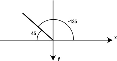
Figure 3-15. Understanding the result of Math.atan2(-2,-2)
Using trig functions for animation
You’ve already seen how sin and cos can be used for making an object move in a circle. They are also especially useful for producing any kind of repeating or oscillating motion. But before we get into animation using trig functions, we need to introduce some new concepts.
Wavelength, period, frequency and angular frequency
Take a look again at Figure 3-12, which shows the graph of the sine function. If x represents distance in space, we have a sine wave in space that repeats at a regular interval. That interval is called the wavelength of the wave. It is the distance between adjacent similar points, for example, the distance between successive crests.
If we instead plot the sine function against time, the repeating interval is a time scale called the period of the wave. For example, if this were a ball that’s moving up and down, the period (denoted by the symbol T) would be the time it takes to return to its initial position. Let’s call this a cycle.
Now, suppose that a cycle takes 0.5 seconds, which we can state as T = 0.5 seconds. How many cycles does the ball complete in 1 second? Well, obviously 2. That’s how many half-seconds there are in a second. This is called the frequency of the motion (denoted by the symbol f).
It is not difficult to see that, in general, the frequency is given by the reciprocal of the period:

Now, it turns out that you can always think of the up-and-down motion of the ball as the projection of the position of another imaginary ball that is moving at a constant rate in a circle (see Figure 3-16). One cycle in an oscillation (wave-like motion) then corresponds to a complete revolution around the circle. Thinking in terms of the angle moved by the circling ball, that’s 2π radians. Because the ball moves f cycles per second, and each cycle is 2π radians, this means that the ball goes through 2πf radians per second. This is called the angular frequency or angular velocity of the motion (usually denoted by the Greek letter ω, omega). It tells you the angle, in radians, through which the circling ball moves in each second.
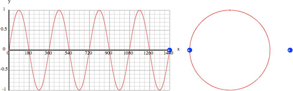
Figure 3-16. Relationship between oscillation, circular motion, and a sine wave
Finally, because ω is the angle through which the imaginary ball moves per second, in t seconds the ball will have moved through ω t radians. So, if it starts out at an angle of 0 radians, at t seconds its projected displacement is equal to sin (ω t):
![]()
If we know the angular frequency of the oscillation, we can calculate the position of the ball at any time if its initial position is known. Of course, if we know the period or frequency instead, we can work out the angular frequency from the preceding formula.
Let’s look at some examples. For these examples, we’re using trig-animations.js, which is a modification of move-curve.js. We will now show, side by side, a 2D animation as well as its 1D version, in which you just move an object along one direction.
Basic oscillations (wave motion in 2D) are pretty straightforward to achieve with just a sine or cosine function. Such an oscillation is called a simple harmonic motion (SHM). The oscillation consists of a wave with a single frequency. Try it out with trig-animations.js:
function f(x){
     var y;
     y = Math.sin(x*Math.PI/180);
     return y;
}
You can produce waves of different frequencies by multiplying the argument by different factors.
Oscillations with a sine wave go on forever. If you want to make them die out with time, you can just multiply the sine by an exponential with a negative coefficient:
y = Math.sin(x*Math.PI/180)*Math.exp(-0.002*x);
You can experiment by changing the coefficient 0.002 to a smaller or larger number. Figure 3-17 shows a typical pattern you might see.

Figure 3-17. Damped oscillations using sin(x) and exp(–x)
Combining sine waves
You can produce all kinds of exotic effects by combining sine and cosine waves. Here’s an example of a combination:
y = Math.sin(x*Math.PI/180) + Math.sin(1.5*x*Math.PI/180);
Or try two sine waves with nearly the same angular frequency:
y = 0.5*Math.sin(3*x*Math.PI/180) + 0.5*Math.sin(3.5*x*Math.PI/180);
This gives you a “beats” motion; a rapid oscillation upon which is superimposed a slower oscillation (see Figure 3-18).

Figure 3-18. Pattern produced by superimposing two sine waves of nearly equal frequency
It is possible to produce all sorts of repeating patterns using a combination of sine waves. There is a mathematical technique called Fourier analysis that allows you to work out what combination of sine waves you need to produce a particular pattern. The resulting sum of sine waves is called a Fourier series.
For example, you can produce something that looks like a square wave (a step function wave) by adding sine waves in the following way:
y = Math.sin(x*Math.PI/180) + Math.sin(3*x*Math.PI/180)/3 + Math.sin(5*x*Math.PI/180)/5;
The more waves you add, the closer the result will be to a square wave. For example, add the next term in the series (Math.sin(7*x*Math.PI/180)/7) to see what you get.
We wrote a little function, fourierSum(N,x), that computes the Fourier sum to N terms for the square wave.
function f(x){
     var y;
     y = fourierSum(10,x);
     return y;
}
function fourierSum(N,x){
     var fs=0;
     for (var nn=1; nn<=N; nn=nn+2){          fs += Math.sin(nn*x*Math.PI/180)/nn;
     }
     return fs;
}
Figure 3-19 shows what you get with N = 10. With a value of N = 1000, the curve is an almost perfect square wave.
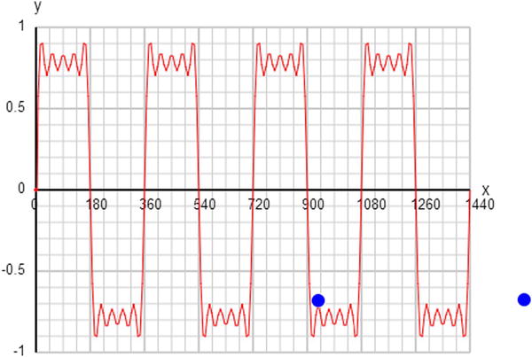
Figure 3-19. Fourier series pattern for a square wave with N = 10
Vectors and basic vector algebra
Vectors are useful math constructs that simplify how we need to deal with many physical quantities like velocity and force, which will be discussed in detail in the next chapter. Vector algebra consists of rules for manipulating and combining vectors. You’ve already met vectors informally, when you dealt with velocity components. Let’s now introduce vectors more formally.
What are vectors?
Vectors can be most intuitively illustrated using the example of displacements. The concept of displacement will be covered in detail in Chapter 4, but essentially it refers to movement for a given distance and in a given direction. Here is an example.
Suppose that Bug, the ladybug, is crawling on a piece of graph paper. Bug starts at the origin and crawls for a distance of 10 units; then he stops. Bug then resumes crawling for a further distance of 10 units before stopping again. How far is Bug from the origin? One might be tempted to say 20 units. But what if Bug crawled upward the first time and to the right the second time? (See Figure 3-20). Clearly 20 units is the wrong answer. By using the Pythagorean Theorem, the answer is actually ![]() , or roughly 14.1 units.
, or roughly 14.1 units.
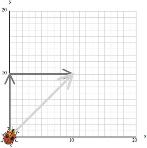
Figure 3-20. The direction of displacement matters!
You can’t simply add the two distances, because you also need to take into account the direction in which Bug moves. To analyze displacements, you need a magnitude and a direction.
In math we abstract this idea into the concept of a vector, which is a quantity that has a magnitude and a direction.
Displacements are not the only vectors. Many of the basic concepts of motion, such as velocity, acceleration, and force, are vectors (they will be discussed in the next chapter). This section outlines the algebra of vectors as abstract mathematical objects, regardless of whether they are displacements, velocities, or forces. With a little grasp of vector algebra, you can simplify calculations by reducing the number of equations that you have to deal with. This saves time, reduces the likelihood of errors, and simplifies life.
Vectors are often contrasted with scalars, which are quantities that have a magnitude only. Distance or length is a scalar—you need only one number to specify it. But displacement is a vector because you need to specify the direction of the displacement. Pictorially, vectors are often represented as directed straight lines—a line with an arrow on it.
Note that a vector is characterized uniquely by its magnitude and direction. That means that two vectors with the same magnitude and direction are considered to be equal, irrespective of where they are in space (see Figure 3-21a). In other words, the location of a vector does not matter. There’s one exception to this rule, however: the position vector. The position vector of an object is the vector that joins a fixed origin to that object, so it’s a displacement vector in relation to a fixed origin (see Figure 3-21b).

Figure 3-21. (a) Parallel vectors of equal length are equal; (b) Position vectors relate to the origin
Adding and subtracting vectors
In the Bug example, what is the sum of the two displacements? The natural answer is that it is the resultant displacement as given by the vector that points from the initial to the final position (refer to Figure 3-20). What if Bug now moves a distance of 5 units downward? You might say that the resultant displacement is the vector that points from the beginning (the origin, in this case) to the destination. This is the so-called head-to-tail rule:
To add two or more vectors, join them so that they are “head-to-tail,” moving them around if necessary (as long as their direction does not change, that is they remain parallel to their original direction). The sum or resultant vector is then the vector that joins the starting point to the ending point.
To subtract a vector from another vector, we just add the negative of that vector. The negative of a vector is one with the same magnitude but pointing in the opposite direction.
Subtracting a vector from itself (or the sum of a vector and its negative) gives you the zero vector—a vector of zero length and arbitrary direction.
Let’s look at an example. Suppose that after Bug has moved 10 units upward, he decides to move 10 units at an angle of 45 degrees instead (see Figure 3-22). What is the resultant displacement? Now that is trickier: you can’t directly apply the Pythagorean Theorem because you don’t have a right triangle any more. You could use some more complicated trigonometry, or draw the vectors accurately and take a ruler and measure the resultant distance and angle.
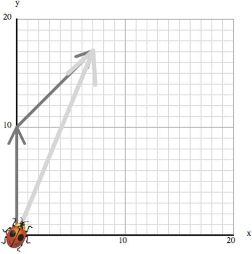
Figure 3-22. Addition of vectors
In practice, that’s not how you’ll be doing it, though. Adding and subtracting vectors is much easier using vector components. So let’s take a look at vector components now.
Resolving vectors: vector components
As mentioned before, a vector has a magnitude and a direction. What this means in 2D is that you need two numbers to specify a vector. Take a look at Figure 3-23. The two numbers are the length r of the vector and the angle θ that it makes with the positive x-axis. But we can also specify the two numbers as the extent of the vector in the x- and y- direction, denoted by x and y respectively. These are called the vector components.
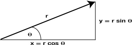
Figure 3-23. Vector components
The relation between (r, θ) and (x, y) can be obtained with the simple trigonometry discussed in the previous section. Looking at Figure 3-23 again, we know this:
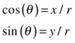
This gives the following:
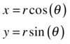
Working out the vector components in this way from the magnitude and angle of a vector is known as “resolving the vector” along the x- and y-axes. Actually, you can resolve a vector along any two mutually perpendicular directions. But most of the time, we’ll be doing that along the x- and y-axes.
There are many different notations for vectors, and it’s easy to get bogged down with notation. But in JavaScript you just have to remember that a vector has components. So any notation that helps you remember that is just as good as any other. We’ll use the following notation for compactness, denoting vectors using bold letters and denoting their components by enclosing them using square brackets:
![]()
In 3D, you need not two, but three, components to specify a vector, so we write this:
![]()
The position vector of an object is a vector pointing from the origin to that object. Hence, we can write the position vector in terms of the coordinates of the object. In 2D:
![]()
In 3D:
![]()
Adding vectors using components
Here’s how you add two vectors using components:
![]()
Pretty simple, isn’t it? Why this is so should be clear from Figure 3-24. You separately add the horizontal components and the vertical components of the two vectors you’re adding. This gives you the components of the resultant vector.
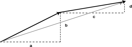
Figure 3-24. Adding vectors using components
As an example, applying this to the Bug displacement problem shown in Figure 3-22 gives the following displacement, which you can easily verify on the graph:
![]()
Feel free to practice doing vector additions with pen and paper; after going through a few, the process should become obvious and help you build your intuition about vectors and vectors components.
Similarly, vector subtraction using components is simply this:
![]()
Multiplying a vector by a number
Multiplying a vector by a number just multiplies each of its components by that number:
![]()
In particular, if we multiply a vector by –1, we get this, which gives the negative of that vector:
![]()
Dividing a vector by a number N is just the same as multiplying the vector by the reciprocal 1/N of that number.
The magnitude (length) of a vector is given by applying the Pythagorean Theorem to its components:
- In 2D, the magnitude of [x, y] is
 ; or in JavaScript code: Math.sqrt(x*x+y*y).
 - In 3D, the magnitude of [x, y, z] is
 ; or in JavaScript code: Math.sqrt(x*x+y*y+z*z).
Note that if we divide a vector by its magnitude, we get a vector of length one unit in the same direction as the original vector. This is called a unit vector.
Calculating the angle of a vector from its components is no more difficult than calculating its magnitude. In JavaScript, this can be done most easily using the Math.atan2() function.
The angle of a vector [x, y] is given by Math.atan2(y, x). Beware—you need to specify the arguments as y first and then x.
Multiplying vectors: Scalar or dot product
Is it possible to multiply two vectors? The answer is yes. Mathematicians have defined a “multiplication” operation called scalar product, in which two vectors produce a scalar. Recall that a scalar only has a magnitude and no direction; in other words, it is basically just a number. The rule is that you multiply the corresponding components of each vector and add the results:
![]()
The scalar product is denoted by a dot, so it is also called the dot product.
Expressed in terms of vector magnitudes and direction, the dot product is given by the following, where θ is the angle between the two vectors, and r1 and r2 are their lengths:
![]()
The geometrical interpretation of the scalar product is that it’s the product of the length of one vector with the projected length of the other (see Figure 3-25).
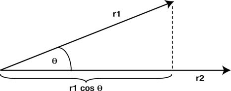
Figure 3-25. The scalar product between two vectors
This is useful when you need to find the angle between two vectors, which you can obtain by equating the right sides of the previous two equations and solving for θ. In JavaScript, you just do this:
angle = Math.acos((x1*x2+y1*y2)/(r1*r2))
Note that if the angle between two vectors is zero (they are parallel), cos (θ) = 1, and the dot product is just the product of their magnitudes.
If the two vectors are perpendicular, then cos (θ) = cos (π/2) = 0, and so the dot product is zero. This is a good test to check if two vectors are perpendicular or not. All these formulas and facts carry over to 3D, with the dot product given by the following:
![]()
Scalar products crop up in several places in physics. We’ll come across an example in the next chapter, with the concept of work, which is defined as the dot product of force and displacement. So, although the dot product may appear somewhat abstract and mysterious as a math construct, it will hopefully make more intuitive sense when you come across it again in an applied context in Chapter 4.
Multiplying vectors: Vector or cross product
In 3D, there is another type of product, known as the vector product because it gives a vector instead of a scalar. The rule is quite a bit trickier.
If you have two vectors a = [x1, y1, z1] and b = [x2, y2, z2], and their vector product is given by a vector c = a ×b = [x, y, z], the components of c are given by the following:

Now this is not exactly intuitive, is it? There sure is some logic to it, as with everything in math. But trying to explain it would be too much of a diversion. So let’s just accept the formula.
The vector product is also called the cross product because of the “cross” notation used to denote it. The vector product of two vectors a and b gives a third vector that is perpendicular to both a and b.
In terms of vector magnitudes and directions, the cross product is given by this:
![]()
where a and b are the magnitudes of a and b respectively, θ is the smaller angle between a and b, and n is the unit vector perpendicular to a and b and oriented according to the right-hand rule (see Figure 3-26): hold your right hand with the forefinger pointing along the first vector a, and your middle finger pointing in the direction of b. Then n will point in the direction of the thumb, held perpendicular to a and b.

Figure 3-26. The right-hand rule for the vector product
Note that the cross product is zero when θ = 0 (because sin (0) = 0). Hence, the cross product of two parallel vectors gives the zero vector.
Like the scalar product, vector products appear in several places in physics; for example in rotational motion.
Building a Vector object with vector algebra
We built a lightweight Vector2D object endowed with all the relevant vector algebra in 2D. Here is the code (see vector2D.js). The method names have been chosen to make intuitive sense.
function Vector2D(x,y) {
     this.x = x;
     this.y = y;
}

// PUBLIC METHODS
Vector2D.prototype = {
     lengthSquared: function(){
          return this.x*this.x + this.y*this.y;
     },
     length: function(){
          return Math.sqrt(this.lengthSquared());
     },
     clone: function() {
          return new Vector2D(this.x,this.y);
     },
     negate: function() {
          this.x = - this.x;
          this.y = - this.y;
     },
     normalize: function() {
          var length = this.length();
          if (length > 0) {
               this.x /= length;
               this.y /= length;
          }
          return this.length();
     },
     add: function(vec) {
          return new Vector2D(this.x + vec.x,this.y + vec.y);
     },
     incrementBy: function(vec) {
          this.x += vec.x;
          this.y += vec.y;
     },
     subtract: function(vec) {
          return new Vector2D(this.x - vec.x,this.y - vec.y);
     },
     decrementBy: function(vec) {
          this.x -= vec.x;
          this.y -= vec.y;
     },
     scaleBy: function(k) {
          this.x *= k;
          this.y *= k;
     },
     dotProduct:     function(vec) {
          return this.x*vec.x + this.y*vec.y;
     }
};

// STATIC METHODS
Vector2D.distance =  function(vec1,vec2){
     return (vec1.subtract(vec2)).length();
}
Vector2D.angleBetween = function(vec1,vec2){
     return Math.acos(vec1.dotProduct(vec2)/(vec1.length()*vec2.length()));
}
The file vector-examples.js contains some examples of the usage of the Vector2D object. You will soon see plenty of examples of its use throughout the book.
Simple calculus ideas
As stated at the beginning of this chapter, we do not assume that all readers will have a background in calculus. If you do, that is certainly handy; but we still recommend that you skim through this section, especially the code examples and the section on discrete calculus, to see how we apply calculus in code. If calculus is completely new to you, this section is designed as a gentle overview of some of the basic concepts. So although you won’t be able to “do” calculus just by reading this section, you will hopefully gain enough understanding to appreciate the meaning of physics formulas that involve calculus. Additionally, you will be introduced to discrete calculus and the subject of numerical methods, which will provide a foundation for approaching more complex physics simulations.
So what is calculus? In one sentence, it’s a mathematical formalism for dealing with quantities that change continuously with respect to other quantities. Because physics deals with laws that relate some quantities to other quantities, calculus is clearly relevant.
Calculus consists of two parts. Differential calculus (or differentiation) deals with the rate of change of quantities. Integral calculus (or integration) deals with continuous sums. The two are related by the fundamental theorem of calculus, which states that integration is the reverse of differentiation.
That all sounds very mysterious if you’ve never come across calculus before, so let’s start from something you know to give you a gentle introduction to the subject. By the end of this chapter, these statements will make much more sense to you.
Slope of a line: gradient
The idea of rate of change is an important concept in physics. If you think of it, we are trying to formulate laws that tell us how, for example, the motion of a planet changes with time; how the force on the planet changes with its position, and so on. The key words here are “changes with.” The laws of physics, it turns out, contain the rate of change of different physical quantities such as position, velocity, and so on.
Informally, “rate of change” tells us how quickly something is changing. Usually we mean how fast it’s changing in time, but we could also be interested in how “fast” something changes with respect to some other quantity, not just time. For example, as a planet moves in its orbit, how quickly does the force of gravity change with its position?
So, in math terms, let’s consider the rate of change of a quantity y with respect to another quantity x (where x could be time t or some other quantity). To do this, we’ll use graphs to help us visualize relationships more easily.
Let’s start with two quantities that have a simple, linear, relationship with each other; that is, they are related by
![]()
As you saw in the coordinate geometry section, this implies that the graph of y against x is a straight line. The constant b is the y-intercept; the point at which the line intersects the y-axis. We’ll now show that the constant a gives a measure of the rate of change of y with x.
Look at Figure 3-27. Of the two lines, in which one is y changing faster with x?
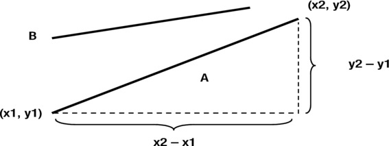
Figure 3-27. The gradient (slope) of a line
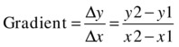
Clearly it’s A, because it is “steeper,” so the same increase in x leads to a larger increase in y. The steepness of the slope of the line therefore gives a measure of the rate of change of y relative to x. We can make this idea precise by defining the rate of change as follows:
Rate of change = (change in y) / (change in x)
It is customary to use the symbol Δ to denote “change in,” so we can write this:
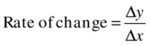
Let’s give the rate of change a shorter name; let’s call it gradient. Here’s the idea: take any two points on the line with coordinates (x1, y1) and (x2, y2), calculate the difference in y and the difference in x and divide the former by the latter:
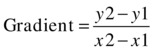
With a straight line, you’ll find that no matter which pair of points you take, you’ll always get the same gradient. Moreover, that gradient is equal to a, the number that multiplies x in the equation y = ax + b.
This makes sense because a straight line has a constant slope, so it should not matter where you measure it. This is a very good start. We’ve got a formula for calculating the gradient or rate of change. The only problem is that it is restricted to quantities that are linearly related to each other. So how do we generalize this result to more general relationships (for example, when y is a nonlinear function of x?)
Rates of change: derivatives
You already know that the graph of a nonlinear function is a curve instead of a straight line. Intuitively, a curve’s slope is not constant—it changes along the curve. Therefore, whatever the rate of change or gradient of a nonlinear function might be, it is not constant but depends on x. In other words, it is also a function of x.
Our objective now is to find this gradient function. In a math course, you’d do some algebra and come up with a formula for the gradient function. For example, you can start with the function y = x2 and show that its gradient function is 2x. But because you’re not in a math course, let’s do that with code instead. But first, we need to define what we mean by the gradient of a curve.
Because the gradient of a curve changes along the curve, let’s focus on a fixed point P on the curve (Figure 3-28).
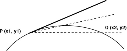
Figure 3-28. The gradient of a curve
Then let’s pick any other point Q near point P. If we draw a line segment joining P and Q, the slope of that line approximates the slope of the curve. If we imagine that Q approaches P, we can expect the gradient of the line segment PQ to be closer and closer to the gradient of the curve at P.
What we are doing, in effect, is using the formula for the gradient of a line we had before and reducing the intervals Δx and Δy:
We can then repeat this process at different locations for the point P along the curve to find the gradient function. Let’s do this now in gradient-function.js:
var canvas = document.getElementById('canvas'),
var context = canvas.getContext('2d'),

var numPoints=1001;
var numGrad=50;
var xRange=6;
var xStep;

var graph = new Graph(context,-4,4,-10,10,275,210,450,350);
graph.drawgrid(1,0.2,2,0.5);
graph.drawaxes('x','y'),
var xA = new Array();
var yA = new Array();
// calculate function
xStep = xRange/(numPoints-1);
for (var i=0; i<numPoints; i++){
     xA[i] = (i-numPoints/2)*xStep;
     yA[i] = f(xA[i]);
}
graph.plot(xA,yA,'#ff0000',false,true); // plot function
// calculate gradient function using forward method
var xAr = new Array();
var gradA = new Array();
for (var j=0; j<numPoints-numGrad; j++){
     xAr[j] = xA[j];
     gradA[j] = grad(xA[j],xA[j+numGrad]);
}
graph.plot(xAr,gradA,'#0000ff',false,true); // plot gradient function

function f(x){
     var y;
     y = x*x;
     return y;
}

function grad(x1,x2){
     return (f(x1)-f(x2))/(x1-x2);
}
The relevant lines are the ones that compute the gradient function, and the function grad(). This function simply computes the gradient (y2 – y1) / (x2 – x1) given x1 and x2 as input. The line that decides which points to use is the following:
gradA[j] = grad(xA[j],xA[j+numGrad]);
Here numGrad is the number of grid points that Q is away from the point P (the point at which we are evaluating the gradient). Obviously, the smaller the value of numGrad, the more accurate the calculated gradient will be.
We have used a total of 1,000 grid points in an x-interval of 6 (from –3 to 3). That gives us a step size of 0.006 units per grid point. Let’s use numGrad=1 to start with. This is the smallest possible value. Running the code plots the gradient function alongside the original function y = x2. The graph of the gradient function is a straight line passing through the origin. When x = 1, y = 2, when x = 2, y = 4, and so on. You can probably guess that the equation of the line is y = 2x. Now any calculus textbook will tell you that the gradient function of y = x2 is y = 2x. So this is good. You’ve successfully calculated your first gradient function!
Now change the value of numGrad to 50. You’ll see that the computed gradient function line shifts a bit; it’s no longer y = 2x. Not too good. Try reducing numGrad. You’ll find that a value of up to about 10 gives you something that looks very close to y = 2x. That’s a step size of 10 × 0.006 = 0.06. Anything much larger than this and you’ll start losing accuracy.
Let’s finish off this section by introducing some more terminology and notation. The gradient function is also called the derived function or derivative with respect to x. We’ll use these terms interchangeably. The process of calculating the derivative is called differentiation.
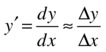
We showed that the ratio Δy/Δx gives the gradient of a curve at a point provided that Δx and Δy are small. In formal calculus, we say that Δy/Δx tends to the gradient function as Δx and Δy go to zero.
To express the fact that the gradient function is really a limiting value of Δy/Δx, we write it like this:
![]()
This is the standard notation for the derivative of function y with respect to x. Another notation is y' (“y prime”); or if we write y = f(x), the derivative can also be denoted by f' (“f prime”).
There is nothing stopping you from calculating the derivative of a derivative. This is called the second derivative, and is written as follows:
![]()
In fact, as you’ll find out in the next chapter, velocity is the derivative of position (with respect to time), and acceleration is the derivative of velocity. So acceleration is the second derivative of position with respect to time. In the notation, v = dx/dt, a = dv/dt, so a = d2x/dt2.
We calculated the derivative of a scalar function, but you can also differentiate vectors. You just find the derivative of each vector component separately.
For example, vx = dx/dt, vy = dy/dt, and vz = dz/dt are the three velocity components. We can write this more compactly in vector form as follows, where v = [vx, vy, vz] and r = [x, y, z]:

Discrete calculus: difference equations
What we did while calculating the gradient function in the preceding code is an example of discrete calculus: calculating the derivative using numerical methods. A numerical method is basically an algorithm for performing a mathematical calculation in an approximate way using code. This is needed if we don’t have an exact formula for the quantity we are calculating.
In the preceding example, we had y = x2 and needed to calculate y' using the discrete form of the derivative:
To do this, we used a difference equation of the following form:
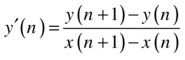
This is called a forward difference scheme because we are calculating the derivative at step n by using values of the function at the next step n+1.
There are many other difference schemes. Let’s try a central difference scheme:
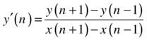
It’s called a central difference scheme because we’re picking a point on either side of the point P at which we’re evaluating the gradient. Here is the code that does this:
// calculate gradient function using centered method
var xArc = new Array();
var gradAc = new Array();
for (var k=numGrad; k<numPoints-numGrad; k++){
     xArc[k-numGrad] = xA[k];
     gradAc[k-numGrad] = grad(xA[k-numGrad],xA[k+numGrad]);
}
If you run this code, you’ll see that it gives you the same answer as the previous scheme for numGrad = 1 (recall that numGrad is the number of grid points between P and Q, and that the smaller it is, the more accurate the computed gradient will be). But if you now try larger values of numGrad, you’ll find that it’s still pretty accurate for a value as large as 250, which amounts to a grid size of 1.5. Compare that with the maximum step size of 0.06 for the forward difference scheme—it’s 25 times larger!
This shows that the central difference scheme is much more accurate than a forward scheme. Figure 3-29 shows the derivatives calculated by the two methods for numGrad = 50. Note that we are plotting two different kinds of things on this graph: the original function y and its gradient function dy/dx. Hence, the labeling on the y-axis. The line that passes exactly through the origin is the gradient function obtained by using the central difference scheme. With your knowledge of coordinate geometry, you should be able to deduce that it’s a plot of the function 2x. In other words, dy/dx = 2x. Anyone who’s done any calculus will instantly recognize 2x as the gradient function of y = x2, our original function—so the central difference scheme is doing very well. The other line, which is computed using the forward difference scheme, has a bit of an offset, though, which means it will have an error associated with it. This is called a numerical integration error. Of course, there is an error associated with all numerical schemes. But in this case, the error due to the central difference scheme is so small that it is not visible on the plot. We’ll go into much more detail on numerical accuracy in Chapter 14.
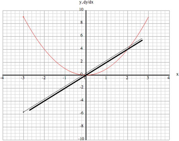
Figure 3-29. Derivatives computed by the forward (thin line) and central (thick line) difference schemes
Doing sums: integrals
Now we ask this question: Is it possible to do the reverse? Suppose we know the derivative of a function; can we find the function? The answer is yes. This is called integration. Again, usually in math you’ll do that using analytical methods. But here we’ll integrate numerically by using code.
As an example of numerical integration, let’s reverse the preceding forward difference scheme to find y(n+1), which gives this:
![]()
Now y' is given, so we can calculate y(n+1) from the previous y(n). So you can see that this will be an iterative process in which we increment the value of y. It’s a sum, and that’s what integration is. The result of integration is called the integral, just as the result of differentiation is called the derivative.
Let’s apply this to the derivative y' = 2x. We should be able to recover the function y = x2. Here’s the code that does this:
var canvas = document.getElementById('canvas'),
var context = canvas.getContext('2d'),

numPoints=1001;
var numGrad=1;
var xRange=6;
var xStep;

var graph = new Graph(context,-4,4,-10,10,275,210,450,350);
graph.drawgrid(1,0.2,2,0.5);
graph.drawaxes('x','y'),
var xA = new Array();
var yA = new Array();
// calculate function
xStep = xRange/(numPoints-1);
for (var i=0; i<numPoints; i++){
     xA[i] = (i-numPoints/2)*xStep;
     yA[i] = f(xA[i]);
}
graph.plot(xA,yA,'#ff0000',false,true); // plot function
// calculate gradient function using forward method
var xAr = new Array();
var gradA = new Array();
for (var j=0; j<numPoints-numGrad; j++){
     xAr[j] = xA[j];
     gradA[j] = grad(xA[j],xA[j+numGrad]);
}
graph.plot(xAr,gradA,'#0000ff',false,true); // plot gradient function
// calculate integral using forward method
var xAi = new Array();
var integA = new Array();
xAi[0] = -3;
integA[0] = 9;
for (var k=1; k<numPoints; k++){
     xAi[k] = xA[k];
     integA[k] = integA[k-1] + f(xA[k-1])*(xA[k]-xA[k-1]);
}
graph.plot(xAi,integA,'#00ff00',false,true); // plot integral

function f(x){
     var y;
     y = 2*x;
     return y;
}
function grad(x1,x2){
     return (f(x1)-f(x2))/(x1-x2);
}
function integ(x1,x2){
     return (f(x1)-f(x2))/(x1-x2);
}
The full source code is in integration.js. One thing you’ll notice is that you have to specify the starting point. This is clear from the preceding equation; because y(n+1) depends on y(n), you need to know the value of y(0) (and x(0)) to begin with. This is called an initial condition. You always have to specify an initial condition when you are integrating. In the code we did that by specifying that x(0) = –3 and y(0) = 9. Try another initial condition and see what you get; for example, x(0) = –3, y(0) = 0.
This example might appear artificial, but in fact it describes an actual physical example: throwing a ball vertically upward. The function f(x) denotes the vertical velocity, and its integral is the vertical displacement. In fact, the derivative f '(x) is the acceleration. If you compute it (as we’ve done in the code), you’ll find that it’s a constant—a straight line with the same value of y for all x, as the acceleration due to gravity is constant. And in case you haven’t guessed what x stands for in this example, it represents time. The initial condition x(0) = –3, y(0) = 9 represents the initial position of the ball. Now it’s clear why you need an initial condition in the first place and why different initial conditions give different curves. Of course, with x representing time, you’d probably start with x(0) = 0. If you feel so inclined, go ahead and animate a ball using the integrated values of y to show that it really produces a ball thrown upward. One thing you’d need to do is to scale y so that it extends over enough pixels on the canvas element.
You could start with the constant acceleration f'(x) and integrate it to get the velocity and then integrate the velocity to get the displacement. In fact, this is what we did, in a simplified way, in the first example of the book: bouncing-ball.js back in Chapter 1.
The forward scheme that we used in both examples (integration.js and bouncing-ball.js) is the simplest integration scheme possible. In Chapter 14, we’ll go into considerable detail on numerical integration and different integration schemes.
Summary
Wow! Well done for surviving this chapter. You now have a remarkable set of tools at your disposal. Hopefully, you can begin to see the potential for applying these ideas and methods. No doubt you have many ideas of your own.
In case you’ve had difficulty with some of the material in this chapter, don’t worry. Things will become much clearer when you see the concepts applied in practice in later chapters. You might want to come back to this chapter again to refresh your memory and reinforce your understanding.
You’re now ready for physics. So take a well-deserved break and, when you feel ready, let’s move on to the next chapter.