![]()
So far in this book you have built simulations in two dimensions. But in the real world there are three dimensions: what does it take to extend the hard work you’ve already done into the 3D realm? In this penultimate chapter we introduce you to the exciting world of 3D physics-based animation.
Topics covered in this chapter include the following:
- 3D physics and math: This section discusses how to extend our existing code framework to create 3D simulations. In the process we’ll explore some additional math concepts that will help to handle both translational and rotational motion in 3D, which will be used in the examples later in the chapter.
- 3D rendering: Introducing WebGL and three.js: This section discusses 3D rendering and the WebGL API, and it introduces the three.js JavaScript library, which simplifies the process of creating 3D simulations with WebGL.
- Simulating particle motion in 3D: This section gives examples of using the three.js library to create physics simulations of particle motion in 3D. The methods used here will then be applied in developing an accurate solar system simulation in Chapter 16.
- Simulating rigid body motion in 3D: Taking a rotating cube as an example, this section shows how to simulate rigid body motion in 3D. In Chapter 16 we will build upon this example to create a flight simulator.
Please note that the focus in this chapter will be very much on doing physics in 3D, rather than on 3D programming in general. Thus, although we’ll inevitably have to discuss some aspects of 3D coding using JavaScript libraries, this chapter is not about the latest cutting-edge 3D technology.
3D physics and math
Before we can create simulations in 3D, we need to generalize some of the math and physics concepts we have been using so far, and introduce new ones along the way.
Most of the physics we’ve discussed so far in this book is essentially unchanged in going from 2D to 3D. The fundamental laws of motion for linear and rotational motion remain the same when expressed in their vector forms. Particle motion is treated in a similar way, with the difference that in 3D particles can move in an extra dimension (that’s obvious, isn’t it?). Hence, the math and code have to be generalized to include the extra space dimension. So we’ll look at vectors and vector algebra in 3D, and construct a Vector3D JavaScript object. We’ll also create a Forces3D object that, together with the Vector3D object, will enable us to write code to handle the motion of particles under a variety of forces in 3D space.
Rigid body dynamics is more complicated because rotation in 3D is complex and requires some more advanced math. So we shall also present the math background needed to handle 3D rotations, introducing new math concepts like matrices and quaternions.
Vectors in 3D
We have used vectors extensively in this book. Just as a reminder of their usefulness, vectors enable the equations that represent physical laws to be written in an economical way. Code written in terms of vector objects is also more concise, more intuitive, and less error-prone. The good news is that vectors in 3D are not very different from their 2D counterparts.
Vectors in 3D are straightforward extensions of their 2D counterparts. In Chapter 3, we reviewed vector algebra in 2D and in 3D side by side. You may wish to read that section again if you need a refresher. The most important difference between vector algebra in 2D and 3D, apart from the obvious fact that there are three components instead of two, is that you can do cross products in 3D.
Back in Chapter 3, we built a Vector2D object that we have steadily been enhancing with new methods. It is straightforward to modify it to create a Vector3D object. The code is in the file vector3D.js downloadable from www.apress.com, and we list it here in full:
function Vector3D(x,y,z) {
     this.x = x;
     this.y = y;
     this.z = z;
}

// PUBLIC METHODS
Vector3D.prototype = {
     lengthSquared: function(){
          return this.x*this.x + this.y*this.y + this.z*this.z;
     },
     length: function(){
          return Math.sqrt(this.lengthSquared());
     },
     clone: function() {
          return new Vector3D(this.x,this.y,this.z);
     },
     negate: function() {
          this.x = - this.x;
          this.y = - this.y;
          this.z = - this.z;
     },
     unit: function() {
          var length = this.length();
          if (length > 0) {
               return new Vector3D(this.x/length,this.y/length,this.z/length);
          }else{
               return new Vector3D(0,0,0);
          }
     },
     normalize: function() {
          var length = this.length();
          if (length > 0) {
               this.x /=length;
               this.y /=length;
               this.z /=length;
          }
          return this.length();
     },
     add: function(vec) {
          return new Vector3D(this.x + vec.x,this.y + vec.y,this.z + vec.z);
     },
     incrementBy: function(vec) {
          this.x += vec.x;
          this.y += vec.y;
          this.z += vec.z;
     },
     subtract: function(vec) {
          return new Vector3D(this.x - vec.x,this.y - vec.y,this.z - vec.z);
     },
     decrementBy: function(vec) {
          this.x -= vec.x;
          this.y -= vec.y;
          this.z -= vec.z;
     },
     multiply: function(k) {
          return new Vector3D(k*this.x,k*this.y,k*this.z);
     },
     addScaled: function(vec,k) {
          return new Vector3D(this.x + k*vec.x, this.y + k*vec.y, this.z + k*vec.z);
     },
     scaleBy: function(k) {
          this.x *= k;
          this.y *= k;
          this.z *= k;
     },
     dotProduct: function(vec) {
          return this.x*vec.x + this.y*vec.y + this.z*vec.z;
     },
     crossProduct: function(vec) {
          return new Vector3D(this.y*vec.z-this.z*vec.y,this.z*vec.x-this.x*vec.z,this.x*vec.y-this.y*vec.x);
     }
};

// STATIC METHODS
Vector3D.distance =  function(vec1,vec2){
     return (vec1.subtract(vec2)).length();
}
Vector3D.angleBetween = function(vec1,vec2){
     return Math.acos(vec1.dotProduct(vec2)/(vec1.length()*vec2.length()));
}
Vector3D.scale = function(vec,sca){
     vec.x *= sca;
     vec.y *= sca;
     vec.z *= sca;
}
The Vector3D methods are straightforward generalizations of their Vector2D counterparts. Note that the crossProduct() method returns a Vector3D object, as it should.
Forces in 3D
Because forces are vector quantities, it won’t surprise you to learn that the newly created Vector3D object makes it a straightforward matter to include forces in 3D simulations.
Newton’s laws of motion in 3D
In Chapter 5, we introduced the laws governing motion, including Newton’s laws of motion. To recap, these laws allow us to compute the motion of objects under the action of forces. If you take a look back at Chapter 5, you will find that these laws were expressed in vector form. Crucially, we did not specify whether we were talking about vectors in 2D or in 3D: the laws are the same. The same is true of the motion concepts we introduced in Chapter 4, such as velocity and acceleration. Therefore, all we have to do when writing 3D code is to define these physical quantities as Vector3D objects instead of Vector2D objects. The laws that we must apply remain the same, and therefore the resulting physics code is virtually identical to its 2D counterpart!
The Forces3D object
Before we can write analogous code for 3D particle motion, we need to update one more key piece of code: the Forces object. Again, this is mostly quite straightforward. We call the new object Forces3D, and list here the code in the corresponding file forces3D.js:
function Forces3D(){
}

// STATIC METHODS
Forces3D.zeroForce = function() {
     return (new Vector3D(0,0,0));
}
Forces3D.constantGravity = function(m,g){
     return new Vector3D(0,m*g,0);
}
Forces3D.gravity = function(G,m1,m2,r){
     return r.multiply(-G*m1*m2/(r.lengthSquared()*r.length()));
}
Forces3D.gravityModified = function(G,m1,m2,r,eps){
     return r.multiply(-G*m1*m2/((r.lengthSquared()+eps*eps)*r.length()));
}
Forces3D.electric = function(k,q1,q2,r){
     return r.multiply(k*q1*q2/(r.lengthSquared()*r.length()));
}
Forces3D.forceField = function(q,E) {
     return E.multiply(q);
}
Forces3D.lorentz = function(q,E,B,vel) {
     return E.multiply(q).add(vel.perp(q*B*vel.length()));
}
Forces3D.central = function(k,n,r) {
     return r.multiply(k*Math.pow(r.length(),n-1));
}
Forces3D.linearDrag = function(k,vel){
     var force;
     var velMag = vel.length();
     if (velMag > 0) {
          force = vel.multiply(-k);
     }else {
          force = new Vector3D(0,0,0);
     }
     return force;
}
Forces3D.drag = function(k,vel) {
     var force;
     var velMag = vel.length();
     if (velMag > 0) {
          force = vel.multiply(-k*velMag);
     } else {
          force = new Vector3D(0,0,0);
     }
     return force;
}
Forces3D.upthrust = function(rho,V,g) {
     return new Vector3D(0,-rho*V*g,0);
}
Forces3D.spring = function(k,r){
     return r.multiply(-k);
}
Forces3D.damping = function(c,vel){
     var force;
     var velMag = vel.length();
     if (velMag>0) {
          force = vel.multiply(-c);
     }
     else {
          force = new Vector3D(0,0,0);
     }
     return force;
}
Forces3D.add = function(arr){
     var forceSum = new Vector3D(0,0,0);
     for (var i=0; i<arr.length; i++){
          var force = arr[i];
          forceSum.incrementBy(force);
          }
     return forceSum;
}
Vectors help us to handle translational motion, whereby an object changes its position in space. You need a more complicated mathematical entity to handle rotations, whereby an extended object changes its orientation in space—you need a matrix.
Introducing matrices
We’ve done a good job of avoiding matrices so far, even when discussing rigid body rotation in Chapter 13. While it was fine to do so in 2D, it is more difficult to ignore matrices in 3D. But before we discuss matrix algebra and rotations in 3D, it would help a lot to do so first in the simpler 2D context.
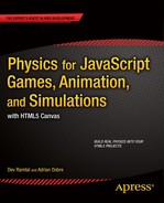
A matrix is essentially an array of numbers, pretty much like a vector. But although a vector is a one-dimensional array, you can have higher-dimensional matrices. We’ll only ever need to worry about two-dimensional matrices, which look something like this:
This matrix has 3 rows and 4 columns; it’s a 3 × 4 matrix. Let’s call it A. Then we can identify particular matrix elements by the row and column number. For example, A(3,2) = –2.
Just like arrays, matrices are useful when you have to deal with a group of similar quantities and you have to perform the same operations on them. They provide a compact way to perform calculations; for example, when you have to do rotations and other transformations. But just as a math vector is more than an array in the sense that it has definite rules for vector algebra (such as vector addition or multiplication), so is a matrix. Let’s take a look at the rules of matrix algebra.
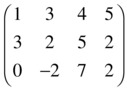
You can add and subtract matrices by adding and subtracting the corresponding elements. This means that you can only add or subtract matrices with the same size, for example for 2 × 2 matrices:
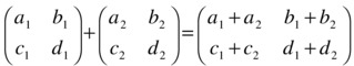
Matrix addition can be applied to represent translations, or displacements, where the position of an object is shifted in space; for example, the following shifts the position of a point by an amount dx and dy along the x and y directions, respectively. This can be represented using 2 × 1 matrices as follows:
Matrix multiplication is a bit more complicated. When you multiply two matrices A and B, you multiply each row of A by each column of B, element by element, and add the results. Here’s an example for 2 × 2 matrices:
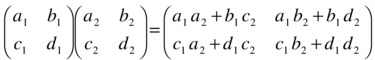
This means that you can only multiply matrix A by matrix B if A has the same number of columns as B has rows. In other words, you can multiply an M × N matrix only by an N × P matrix.
Note that multiplying the mth row by the nth column gives you the (m,n) matrix element in the product. Also, the result of multiplying an M × N matrix by an N × P matrix is an M × P matrix.
Matrix multiplication can transform objects in all sorts of ways, depending on the form of the matrix we’re multiplying with. We’re especially interested in rotation matrices.
Matrices are especially useful for doing rotations. To see this, let’s say you have an object that you want to rotate through an angle θ about an axis perpendicular to the xy plane through the origin (see Figure 15-1). Let’s use the math coordinate system so that the y -axis points upward and angles are measured in a counterclockwise sense.
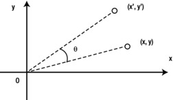
Figure 15-1. Rotating an object in 2D
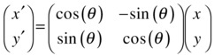
Using trigonometry, you can show that each point on the object with coordinates (x, y) will be moved to a new position with coordinates (x’, y’) given by the following equations:

By the way, this is the math behind the rotate() method of the Vector2D object that we introduced in Chapter 13. You can represent this relationship between the new and old coordinates as a single matrix equation:
What we have done here is to represent each of the position vectors r and r’ of points (x, y) and (x’, y’) as a matrix with a single column (called a column matrix or column vector). If you multiply out the matrices on the right side and equate the elements of the resulting column vector with those on the left side of the equation, you will recover the previous two equations.
We can write this matrix equation in a convenient shorthand form as follows:
![]()
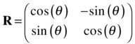
The matrix R is called the rotation matrix and is given by the following:
Instead of rotating the object, you could also rotate the coordinate system (axes):

What’s happening here is that rotating the coordinate axes by angle θ is the same as rotating the object by angle –θ. So, if you replace θ by –θ in the original matrix and use the fact that sin (–θ) = –sin (θ), and cos (–θ) = cos (θ), you end up with the second matrix. So, the rule for swapping between object and coordinate system rotations is to “reverse the signs of the sines.”
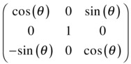
In 3D, the situation is complicated by the fact that you have three components and also three independent directions about which you can perform rotations. The rotation matrix is a 3 × 3 matrix, and for rotation about the z-axis it is given by this:

The rotation matrix about the x-axis is given by this:
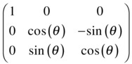
A rotation about the y-axis is given by this matrix:
As in the 2D case, the signs of the sines are reversed if the coordinate axes are rotated instead.
Rotation matrices can be combined by multiplying them together. So a rotation with matrix R1 followed by a rotation with matrix R2 is equivalent to a rotation with matrix R2R1. Note that the order of the rotation matters in 3D. For example, rotating a cuboid by 90° clockwise about the x-axis and then 90° clockwise about the z-axis will have the cuboid end up in a different orientation than a corresponding rotation about the z-axis followed by a rotation about the x-axis. Try it with a book! Mathematically, this corresponds to the fact that matrix multiplication is not commutative. In other words:
![]()
On the other hand, very small incremental (infinitesimal) rotations are commutative, so it does not matter in what order infinitesimal rotations about different axes are performed. This has important implications for how we can represent angular orientation and angular velocity in 3D. The noncommutativity of rotations about the x-, y-, and z-axes means that there is no unambiguous meaning to angular orientation as a vector with three components. So you cannot form a true vector from angular rotation θ in 3D. However, you can form a vector for small angular increments Δθ and therefore for angular velocity ω = dθ/dt.
As the preceding discussion has shown, rotation matrices are very useful mathematical objects that can be implemented in code to allow objects to be rotated in 3D. However, in practice dealing with matrix operations is generally not very efficient from a computational point of view. Without going into details, suffice it to say that a 3 × 3 matrix has nine components, and matrix operations such as multiplication involve a lot of calculations, some of which are redundant. Fortunately, there is a more efficient method to perform rotations in 3D—using even more exotic math objects known as quaternions.
Quaternions
The most convenient way to handle rotations in 3D involves the use of quaternions, which belong to an abstract number system. These rather mysterious mathematical entities are not frequently covered in college or university math courses—so chances are you may not have come across them before. Let’s therefore spend a little time on an informal introduction to quaternions.
Introducing quaternions
Quaternions were invented by an Irish mathematician named William Hamilton in the nineteenth century as an extension of the so-called complex (or imaginary) numbers. As you might imagine, this makes them rather abstract constructs. For our purposes, it is more useful to think of a quaternion as a combination of a scalar and a vector (see Chapter 3 for a refresher on scalars and vectors). We can write a quaternion symbolically as
![]()
Where s is the scalar part and v is the vector part. We can also write the vector components explicitly, like this:
![]()
There are alternative notations, but this is probably the simplest. In this notation, it is tempting to think of a quaternion as a vector with four components. For many purposes this is quite helpful, as long as you keep in mind that the rules for manipulating and combining quaternions (that is, quaternion algebra) are somewhat different from those of vectors. Let’s take a look at quaternion algebra now.
Quaternion algebra
The operations that you will need to know for handling 3D rotations are addition of two quaternions, multiplication of a quaternion by a scalar, and multiplication of two quaternions. Additionally, you will need to know about the magnitude of a quaternion, the conjugate and inverse of a quaternion, and the identity quaternion.
To add or subtract two quaternions, you simply add or subtract their respective components:
![]()
To multiply or divide a quaternion by a scalar, you multiply or divide each of the components of the quaternion by the scalar:
![]()
The previous rules are similar to those for combining vectors. To multiply a quaternion by another quaternion is more complicated and is done using a combination of the dot and cross products. It is most conveniently written in terms of the following notation:
![]()
Note that quaternion multiplication is not commutative—the order of multiplication matters.
The identity quaternion is a special quaternion with a scalar part equal to unity and a vector part equal to zero: 1 = (1,0,0,0). It is so called because multiplying any quaternion by the identity quaternion leaves it unchanged (we leave the proof as an exercise!).
The magnitude or norm of a quaternion q = (s,v1,v2,v3) is defined in a similar way to that of a vector:
![]()
Dividing a quaternion by its magnitude gives a quaternion of unit magnitude, also called a unit quaternion. This process is called normalization.
For any quaternion q = (s,v1,v2,v3) there is a conjugate quaternion defined by q* = (s,–v1,–v2,–v3). It is easy to show that the product of a quaternion and its conjugate gives a quaternion with a zero vector part and with a scalar part equal to the norm squared of the quaternion (again, we leave this as an exercise):
![]()
The inverse q–1 of a quaternion q is equal to its conjugate divided by the square of its norm:

Multiplying a quaternion with its inverse gives the identity quaternion:
![]()
Like matrices, quaternions can be used for rotating vectors. In the previous section we saw that a rotation matrix R transforms a vector r to a vector r’ according to the formula r’ = R r. That is, we simply premultiply the vector by the rotation matrix to get the rotated vector. The equivalent formula for rotating a vector r with a quaternion q is a little more complicated:
![]()
Here r is a quaternion with a scalar part of zero and with the vector part equal to r: r = (0,r).
If q is a unit quaternion, then that is the same as the following equation:
![]()
In this case, the rotation quaternion can always be written in the following form, to represent a rotation through an angle θ around an axis represented by the unit vector u:
![]()
Like rotation matrices, two rotation quaternions q1 and q2 can be combined by multiplying (or composing) them together to give a quaternion q’ representing the combined rotation:
![]()
This represents a rotation represented by q1 followed by one represented by q2. Recall that quaternion multiplication is not commutative, so the order of the product will give different rotations in 3D space.
Rotational dynamics in 3D
The final piece of background theory you need is about how to implement rigid body dynamics in 3D. To do this, we first need to establish how key concepts such as angular orientation, angular velocity, torque, and so on generalize to 3D.
In 2D the orientation of an object can be straightforwardly described by an angle in the x–y plane, which can be interpreted as a rotation about a virtual z–axis perpendicular to that plane. It is tempting to generalize this method to 3D by specifying orientation as a combination of rotations through angles about the x, y, and z axes. These angles are known as Euler angles. Unfortunately there are serious problems with this approach. First, as discussed in the section “Rotation matrices in 3D”, the orientation of an object as defined in this way would depend on the order of the rotations about the three axes. This is hardly satisfactory. Second, certain configurations can result in the dreaded “gimbal lock” problem, whereby no rotation is possible about one of the axes (search for “gimbal lock” on the Web for more details); this proved to be an issue during the Apollo 11 mission.
A better solution is to use a rotation matrix to characterize orientation—because a rotation matrix tells us how to rotate an object with respect to a fixed set of axes, it can also be thought of as holding information on the orientation of the rotated object. The problem then becomes one of computing the evolution in time of the rotation matrix. This is certainly doable and is a very common method of animating rotations. But it suffers from the slight disadvantage that one has to deal with matrix algebra, which is not generally computationally efficient.
Our preferred method is to use a unit quaternion to represent orientation. This is possible for the same reason that a rotation matrix can be used to represent orientation. To illustrate how that might work, suppose the initial orientation of a rigid body is described by a unit quaternion q. We then subject the rigid body to a rotation described by a unit quaternion p. The new orientation q’ of the rigid body is then obtained simply by multiplying q by p:
![]()
The question we face in a physics animation is: how do we find the quaternion p that we need to multiply q with at each timestep? In discrete form, we are looking for p such that:
![]()
Time to go back to angular velocity.
Angular velocity and orientation
In the section “Rotation matrices in 3D” we made the point that an infinitesimal angular displacement is a vector, and hence so is the angular velocity ω = dθ/dt. It turns out that there is a particularly simple evolution equation relating the orientation quaternion with the angular velocity. In a coordinate frame attached to a rotating object (the so-called body frame), it can be written as:

Here ω is the angular velocity quaternion, constructed by setting the vector part of the quaternion equal to the angular velocity vector and the scalar part to zero. This equation tells us how the orientation quaternion q of an object changes in time: its rate of change is equal to half the product of q and the angular velocity ω.
To apply this equation in code, we first have to discretize it. Using the Euler method we can write:
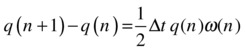
Rearranging, we can write this equation as:
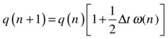
This equation relates the orientation quaternion at the new timestep q(n+1) to that at the old timestep q(n). The quantity in the square brackets is the expression for p(n) that we were looking for. This is the rotation quaternion by which we need to multiply q at each timestep to update the orientation. Note that the first 1 in the square brackets denotes the identity quaternion.
A key requirement is that q must be a unit quaternion at all times; otherwise, the object will be scaled or distorted as the animation progresses. Because there will inevitably be numerical errors that will accumulate over time and cause the norm of q to deviate from unity, it is wise to normalize q frequently, possibly at every timestep.
Torque, angular acceleration, and the moment of inertia matrix
Just like angular velocity, angular acceleration, α = dω/dt, is also a vector in 3D. A rigid body will experience an angular acceleration if there is a resultant torque T acting on it. In 3D the angular equation of motion can be written in the body frame as the following matrix equation:
![]()
Recall that torque is given by the cross product of the position vector of the point of application of a force from the center of rotation and the force vector: T = r × F. This equation can be solved numerically to give the angular velocity at each timestep. The additional complication is that in 3D the moment of inertia I is a 3 × 3 matrix. In the special case where I is diagonal and the diagonal elements are all equal, Ixx = Iyy = Izz = I, the previous equation simplifies to T = I α, similar to the 2D case in Chapter 13.
3D rendering: Introducing WebGL and three.js
After this fairly lengthy introduction to 3D math and physics, you are no doubt impatient to see it all in action. But how do you produce 3D graphics and animation in the browser? It’s time to introduce WebGL and three.js.
Canvas, WebGL, and WebGL frameworks
The HTML5 canvas element is an inherently 2D environment. So how can we extend its capabilities to render 3D? It is possible to simulate 3D on a 2D canvas by applying perspective distortion—this is sometimes known as 2.5D. This is the approach taken in the book Foundation HTML5 Animation with JavaScript by Billy Lamberta and Keith Peters. However, it is a rather laborious process, and there are issues with performance. Fortunately, there is now an easier and more powerful alternative—WebGL.
WebGL: extending canvas to 3D
WebGL originated from attempts at Mozilla to add 3D capabilities to the canvas element. It is essentially a JavaScript API for rendering both 2D and 3D graphics within the web browser. WebGL is based on OpenGL ES 2.0 and allows GPU (Graphics Processing Unit) acceleration in compatible browsers. At the time of this writing, WebGL is now supported by most of the major web browsers. To check if your browser or device supports WebGL, you can visit one of the following web sites:
http://webglreport.com/
http://get.webgl.org/
A WebGL program consists of JavaScript control code and shader code executed on a computer’s GPU (a shader is a program that performs shading of 3D models for depth perception and visual effects). Coding in pure WebGL can be a rather laborious process and is outside the scope of this book. Instead, we shall make use of a framework that will avoid the need to write raw shader code altogether.
So far we’ve done very well without needing to use external libraries or frameworks. But we’ll make an exception for 3D, as we’re not particularly keen on spending hours with low-level WebGL commands! There are a number of JavaScript frameworks and libraries that build on top of WebGL to simplify the process of coding in 3D. Three.js and babylon.js are just two among the more popular ones. In this book we will use the three.js library.
A quick three.js primer
The purpose of this section is to present the absolute minimum you need to know to get up and running with three.js. There are many books and online sources on three.js that we encourage you to consult if you want to get a more in-depth knowledge. The first place to head to is, of course, the official project web page at http://three.org, where you will find documentation and examples, and will be able to download the latest version of the library. For convenience we have included a copy of the three.min.js file, which contains the full library, in the downloadable source code for this chapter. Needless to say, you will have to include this file in a <script> tag in your HTML files in all the examples in this chapter.
The renderer
First you need to choose a renderer. You have a choice of renderers, including a CanvasRenderer and the much better-performing WebGLRenderer, which uses the GPU. You can create a WebGLRenderer and add it to the DOM with the following lines of code:
var renderer = new THREE.WebGLRenderer();
renderer.setSize(window.innerWidth, window.innerHeight);
document.body.appendChild(renderer.domElement);
The last line creates a canvas element that will display the scene.
The scene
A scene sets an area where visual elements, cameras, lights, and so on can be placed. Creating a scene couldn’t be simpler:
var scene = new THREE.Scene();The camera
Next you need a camera. There are different choices of camera available, and we refer you to the documentation for details. Here we just pick a PerspectiveCamera, set its position, and add it to the scene thus:
var camera = new THREE.PerspectiveCamera(45, window.innerWidth/window.innerHeight, 0.1, 10000);
camera.position.set(100,0,400);
scene.add(camera);
You need to specify four arguments in PerspectiveCamera: fov (field of view), aspect, near, and far. The field of view is here set at 45 degrees, and the aspect ratio as the ratio between the browser window’s width and height. The near and far parameters are respectively the closest and farthest distance at which the camera will render objects (here set at 0.1 and 10000).
The second line of code in the previous listing sets the position of the camera using (x,y,z) coordinates. The last line adds the camera to the scene.
Lighting
You need a light to see the objects on the scene. Several different choices are possible (see the documentation), and you can use more than one light. Let’s pick a DirectionalLight:
var light = new THREE.DirectionalLight();
light.position.set(-10,0,20);
scene.add(light);
Objects: mesh, geometry, and material
Next you need to populate the scene with one or more objects. In three.js, you create an object with a Mesh, which takes two arguments, Geometry and Material. Again, there are many choices of Geometry and Material depending on the shape and appearance of the objects you want to create. Let’s create a sphere and give it a MeshLambertMaterial with a red color:
var sphereGeometry = new THREE.SphereGeometry(50,20,20);
var sphereMaterial = new THREE.MeshLambertMaterial({color: 0xff0000});
var ball = new THREE.Mesh(sphereGeometry,sphereMaterial);
ball.position.set(100,0,0);
scene.add(ball);
The SphereGeometry takes three arguments: radius, number of horizontal segments (similar to latitude lines), and number of vertical segments (similar to longitude lines).
The 3D coordinate system
In WebGL and three.js the coordinate system is as shown in Figure 15-2. The x-axis points from left to right, the y-axis from bottom to top, and the z-axis points out of the screen. The origin is at the center of the display area. The location of the origin and the direction of the y-axis are different than in the 2D canvas coordinate system. These differences must be taken into consideration in your code.
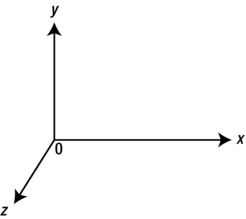
Figure 15-2. The 3D coordinate system
Animation with three.js
To animate objects in 3D using three.js is essentially the same as in 2D. You first create an animation loop using any of the methods described in Chapter 2 and used throughout the book. Within the animation loop you then update the position and/or orientation of objects at each timestep.
You have already seen how the position of an object (obj say) can be set using the obj.position.set() method. You can also set or update individual coordinates separately, as in this example:
obj.position.x = 100;
In three.js, an object’s orientation can be specified by a rotation property, which is an Euler angle representation with three components x, y, and z. For example:
obj.rotation.y = Math.PI/2;
It is also possible to specify an object’s orientation using its quaternion property. You will see an example in the section “Simulating rigid body motion in 3D.”
Simulating particle motion in 3D
Okay, after all this background material, it’s finally time for some code examples. Let’s start with our “hello world” physics simulation—a bouncing ball!
A bouncing ball simulation in 3D
Because this is our first 3D example, it is useful to see the code in full. The code is in bouncing-ball.js and is listed here:
var width = window.innerWidth, height = window.innerHeight;
var scene, camera, renderer;
var ball;
var t0, dt;
var g = -20;
var fac = 0.9;
var radius = 20;
var x0 = -100, y0 = -100, z0 = -100;

window.onload = init;

function init() {
     renderer = new THREE.WebGLRenderer();
     renderer.setSize(width, height);
     document.body.appendChild(renderer.domElement);

     scene = new THREE.Scene();

     var angle = 45, aspect = width/height, near = 0.1, far = 10000;
     camera = new THREE.PerspectiveCamera(angle, aspect, near, far);
     camera.position.set(100,0,400);
     scene.add(camera);

     var light = new THREE.DirectionalLight();
     light.position.set(-10,0,20);
     scene.add(light);

     var sphereGeometry = new THREE.SphereGeometry(radius,20,20);
     var sphereMaterial = new THREE.MeshLambertMaterial({color: 0x006666});
     ball = new THREE.Mesh(sphereGeometry,sphereMaterial);
     scene.add(ball);
     ball.pos = new Vector3D(100,0,0);
     ball.velo = new Vector3D(-20,0,-20);
     positionObject(ball);

     var plane1 = new THREE.Mesh(new THREE.PlaneGeometry(400, 400), new THREE.MeshNormalMaterial());
     plane1.rotation.x = -Math.PI/2;
     plane1.position.set(0,y0,0);
     scene.add(plane1);

     var plane2 = new THREE.Mesh(new THREE.PlaneGeometry(400, 400), new THREE.MeshNormalMaterial());
     plane2.position.set(0,0,z0);
     scene.add(plane2);

     var plane3 = new THREE.Mesh(new THREE.PlaneGeometry(400, 400), new THREE.MeshNormalMaterial());
     plane3.rotation.y = Math.PI/2;
     plane3.position.set(x0,0,0);
     scene.add(plane3);

     t0 = new Date().getTime();
     animFrame();
}

function animFrame(){
     requestAnimationFrame(animFrame);
     onTimer();
}
function onTimer(){
     var t1 = new Date().getTime();
     dt = 0.001*(t1-t0);
     t0 = t1;
     if (dt>0.2) {dt=0;};
     move();
}
function move(){
     moveObject(ball);
}
function positionObject(obj){
     obj.position.set(obj.pos.x,obj.pos.y,obj.pos.z);
}
function moveObject(obj){
     obj.velo.y += g*dt;
     obj.pos = obj.pos.addScaled(obj.velo,dt);
     if (obj.pos.x < x0 + radius){
          obj.pos.x = x0 + radius;
          obj.velo.x *= -fac;
     }
     if (obj.pos.y < y0 + radius){
          obj.pos.y = y0 + radius;
          obj.velo.y *= -fac;
     }
     if (obj.pos.z < z0 + radius){
          obj.pos.z = z0 + radius;
          obj.velo.z *= -fac;
     }
     positionObject(obj);
     renderer.render(scene, camera);
}
We begin by storing the width and height of the browser window in the variables width and height, which we’ll use in a couple of places. Then we create variables for the scene, camera, and renderer, and a ball object. The radius of the ball is stored in the variable radius, which we’ll use in a number of places. Note that the variable g, which represents acceleration due to gravity, is given a negative value. The reason is that WebGL’s vertical (y) axis points upward rather than downward.
In the init() method we set up the renderer, scene, camera, and light as discussed in the previous section. We then create a ball using SphereGeometry. Next we create new properties pos and velo for the ball object and assign them Vector3D values to hold its initial position and velocity. Note that you must include the vector3D.js file in your HTML file. The ball.pos and ball.velo variables will be used for performing the physics calculations. But we also need to tell WebGL to set the ball’s position on the canvas each time these variables are updated. This is done by calling the positionObject() method, which updates the position property of the ball using the pos values:
function positionObject(obj){
     obj.position.set(obj.pos.x,obj.pos.y,obj.pos.z);
}
Next in init(), we create three walls using the PlaneGeometry object, and orient and position them suitably using the rotation and position properties of the instances.
The animation code looks very similar to what you are already used to for creating 2D canvas simulations. The new pieces of code are in the moveObject() method. In the first two lines we update the vertical velocity and the position vector of the ball. Then we check for collisions with each of the three walls in a similar way to what we did in the very first example in Chapter 1. We then call positionObject() to update the position property of the ball before rendering the scene.
Run the code and you should see something similar to the screenshot in Figure 15-3. As ever, feel free to experiment by changing the parameters and visual elements.
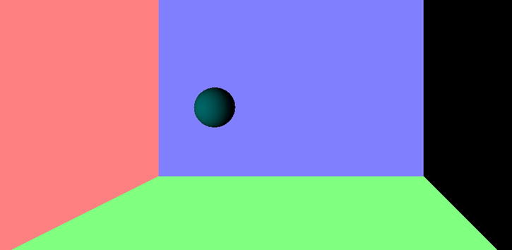
Figure 15-3. Bouncing ball in 3D
A rotating Earth animation
Creating rotating animations is easily achieved with three.js. To illustrate how to do it, let’s make a rotating Earth animation. The code for this example is actually simpler than the previous example, and you’ll find it in the file earth.js. Here is the full listing:
var width = window.innerWidth, height = window.innerHeight;
var renderer = new THREE.WebGLRenderer();
renderer.setSize(width, height);
document.body.appendChild(renderer.domElement);

var scene = new THREE.Scene();

var angle = 45, aspect = width/height, near = 0.1, far = 10000;
var camera = new THREE.PerspectiveCamera(angle, aspect, near, far);
camera.position.set(100,0,500);
scene.add(camera);

var light = new THREE.DirectionalLight();
light.position.set(-10,0,20);
scene.add(light);

var radius = 100, segments = 20, rings = 20;
var sphereGeometry = new THREE.SphereGeometry(radius,segments,rings);
var sphereMaterial = new THREE.MeshLambertMaterial();
sphereMaterial.map = THREE.ImageUtils.loadTexture('images/earth.jpg'),
var sphere = new THREE.Mesh(sphereGeometry,sphereMaterial);
scene.add(sphere);

function animFrame(){
     requestAnimationFrame(animFrame);
     onEachStep();
}
function onEachStep() {
     sphere.rotation.y += 0.01;
     camera.position.z -= 0.1;
     renderer.render(scene, camera);
}
animFrame();
As you can see, we have simplified the animation code considerably. Aside from this, the novelty lies in just three lines of code, which appear in boldface type. The first line loads an image that it uses as a texture map for the SphereGeometry object created, giving the appearance of a 3D Earth that you can see in Figure 15-4. Note that your code may not work properly if you simply open the HTML file in a web browser, because of a security feature in JavaScript that stops externally hosted files from loading. If that happens, a helpful three.js page at https://github.com/mrdoob/three.js/wiki/How-to-run-things-locally explains how to circumvent the problem.

Figure 15-4. Rotating Earth in 3D
In the function onEachStep(), the first two lines increment the y component of the rotation property of the Earth and decrement the z component of the camera’s position. Run the code to see the resulting effect.
Forces: gravity and orbits in 3D
Next, we’ll add a Moon and some gravity physics to make it orbit the Earth! We will need accurate time-keeping, so will restore the full animation loop that we’ve used for most of the examples in the book. You will also need to add the forces3D.js file in your HTML file.
The resulting code is in earth-moon.js and is reproduced here:
var width = window.innerWidth, height = window.innerHeight;
var acc, force;
var t0, dt;
var animId;
var G = 1;
var M = 50000;
var m = 1;
var scene, camera, renderer;
var earth, moon;

window.onload = init;

function init() {
     renderer = new THREE.WebGLRenderer();
     renderer.setSize(width, height);
     document.body.appendChild(renderer.domElement);

     scene = new THREE.Scene();

     var angle = 45, aspect = width/height, near = 0.1, far = 10000;
     camera = new THREE.PerspectiveCamera(angle, aspect, near, far);
     camera.position.set(0,100,1000);
     scene.add(camera);

     var light = new THREE.DirectionalLight();
     light.position.set(-10,0,20);
     scene.add(light);

     var radius = 100, segments = 20, rings = 20;
     var sphereGeometry = new THREE.SphereGeometry(radius,segments,rings);
     var sphereMaterial = new THREE.MeshLambertMaterial({color: 0x0099ff});
     sphereMaterial.map = THREE.ImageUtils.loadTexture('images/Earth.jpg'),
     earth = new THREE.Mesh(sphereGeometry,sphereMaterial);
     scene.add(earth);
     earth.mass = M;
     earth.pos = new Vector3D(0,0,0);
     earth.velo = new Vector3D(0,0,0);
     positionObject(earth);

     moon = new THREE.Mesh(new THREE.SphereGeometry(radius/4,segments,rings),new THREE.MeshLambertMaterial());
     scene.add(moon);
     moon.mass = m;
     moon.pos = new Vector3D(300,0,0);
     moon.velo = new Vector3D(0,0,-12);
     positionObject(moon);

     t0 = new Date().getTime();
     animFrame();
}

function animFrame(){
     requestAnimationFrame(animFrame);
     onTimer();
}
function onTimer(){
     var t1 = new Date().getTime();
     dt = 0.001*(t1-t0);
     t0 = t1;
     if (dt>0.2) {dt=0;};
     move();
}
function move(){
     positionObject(moon);
     moveObject(moon);
     calcForce(moon);
     updateAccel(moon);
     updateVelo(moon);
}
function positionObject(obj){
     obj.position.set(obj.pos.x,obj.pos.y,obj.pos.z);
}
function moveObject(obj){
     obj.pos = obj.pos.addScaled(obj.velo,dt);
     positionObject(obj);
     earth.rotation.y += 0.001;
     renderer.render(scene, camera);
}
function calcForce(obj){
     var r = obj.pos.subtract(earth.pos);
     force = Forces3D.gravity(G,M,m,r);
}
function updateAccel(obj){
     acc = force.multiply(1/obj.mass);
}
function updateVelo(obj){
     obj.velo = obj.velo.addScaled(acc,dt);
}
You should be able to follow this code without any difficulty. The init() method sets up the scene and 3D objects, and the animation code works as in the 2D examples, substituting Vector3D variables for Vector2D ones as needed.
Run the code and you will be treated to a visually appealing 3D simulation of the Moon orbiting the Earth, as shown in Figure 15-5. You can change the position of the camera to view the system from different points of view. For example, add the following line in init() to view the Moon from the Earth’s position:
camera.position = earth.position;
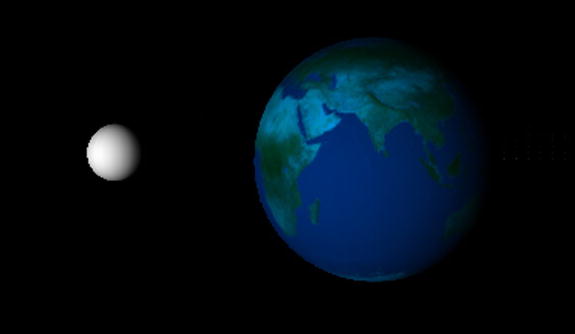
Figure 15-5. Earth-Moon simulation
Or add the following line in moveObject() to view the Earth from the Moon:
camera.position = moon.position;
We leave you to develop the code further and add interactivity, for example to change the camera location or add zooming effects and so on.
Needless to say, the simulation is not to scale, but it does contain the essential physics. In Chapter 16, you will build an accurate and much more realistic simulation of the solar system.
Simulating rigid body motion in 3D
We are now ready to simulate rigid body motion in 3D. Let us choose a simple object–a rotating cube–for which the moment of inertia matrix has equal diagonal elements and the nondiagonal elements equal to zero. As we saw in the section “Rotational dynamics in 3D,” the relationship between torque and angular acceleration then simplifies to T = I α, where I is the value of each diagonal element of the moment of inertia matrix.
As a starting point, let us go back to the rigid-body-dynamics.js simulation of Chapter 13 and make a few modifications to replace the rotating square we had there with a rotating cube. The modified code is in cube-rotation.js and is reproduced here in full:
var width = window.innerWidth, height = window.innerHeight;
var t0, dt;
var cube;
var scene, camera, renderer;
var alp, torque;
var t0, dt;
var animId;
var k = 0.5; // angular damping factor
var tqMax = 2;
var tq = 0;

window.onload = init;

function init() {
     renderer = new THREE.WebGLRenderer();
     renderer.setSize(width, height);
     document.body.appendChild(renderer.domElement);

     scene = new THREE.Scene();

     var angle = 45, aspect = width/height, near = 0.1, far = 10000;
     camera = new THREE.PerspectiveCamera(angle, aspect, near, far);
     camera.position.set(100,0,500);
     scene.add(camera);

     var light = new THREE.DirectionalLight();
     light.position.set(30,0,30);
     scene.add(light);

     cube = new THREE.Mesh(new THREE.CubeGeometry(100, 100, 100), new THREE.MeshNormalMaterial());
     cube.overdraw = true;
     scene.add(cube);
     cube.im = 1;
     cube.angVelo = 0;

     addEventListener('mousedown',onDown,false);
     t0 = new Date().getTime();
     animFrame();
}
function onDown(evt){
     tq = tqMax;
     addEventListener('mouseup',onUp,false);
}
function onUp(evt){
     tq = 0;
     removeEventListener('mouseup',onUp,false);
}
function animFrame(){
     animId = requestAnimationFrame(animFrame);
     onTimer();
}
function onTimer(){
     var t1 = new Date().getTime();
     dt = 0.001*(t1-t0);
     t0 = t1;
     if (dt>0.2) {dt=0;};
     move();
}
function move(){
     moveObject(cube);
     calcForce(cube);
     updateAccel(cube);
     updateVelo(cube);
}
function moveObject(obj){
     obj.rotation.x += obj.angVelo*dt;
     renderer.render(scene, camera);
}
function calcForce(obj){
     torque = tq;
     torque += -k*obj.angVelo; // angular damping
}
function updateAccel(obj){
     alp = torque/obj.im;
}
function updateVelo(obj){
     obj.angVelo += alp*dt;
}
In the init() method, we have added new code to set up the scene and related objects with the help of three.js commands. We then create a cube with CubeGeometry and give it new properties of im (moment of inertia) and angVelo (angular velocity), with values set to 1 and 0 respectively. The animation part of the code closely follows that in the rigid-body-dynamics.js code of Chapter 13. Here we have removed bits of code relating to forces, as we are only applying a torque and no force. For simplicity, both the torque and the angular acceleration are treated as scalars, exactly as they are in the 2D case. This is fine for now, as we shall rotate the cube about either the x-, y-, or z-axis. In the code listing we have the following line, which makes the cube rotate around the x–axis:
obj.rotation.x += obj.angVelo*dt;
You can change this line to rotate about one of the other two axes instead. There are event listeners and handlers that apply a constant torque that makes the cube rotate when you click the mouse, and set the torque to zero otherwise. An angular damping term has been included as in the 2D example. Run the code and click the mouse to experiment with the simulation. A screenshot is shown in Figure 15-6.
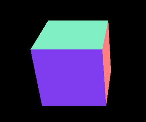
Figure 15-6. A rotating cube in 3D
Applying a force to the rotating cube
Let us now develop the rotating cube simulation further by treating the torque and the angular acceleration as vectors instead of scalars. In this example we’ll handle the rotation using Euler angles. We’ll also include code to deal with forces. To compensate for the increased length of the code, we remove the event handlers and listeners, thus losing interactivity. The new code (cube-euler-angles.js) now looks like this:
var width = window.innerWidth, height = window.innerHeight;
var t0, dt;
var cube;
var scene, camera, renderer;
var acc, force;
var alp, torque;
var t0, dt;
var animId;
var k = 0.5;
var kSpring = 0.2;
var tq = new Vector3D(1,0,0);
var center = new Vector3D(0,0,-500);

window.onload = init;

function init() {
     renderer = new THREE.WebGLRenderer();
     renderer.setSize(width, height);
     document.body.appendChild(renderer.domElement);

     scene = new THREE.Scene();

     var angle = 45, aspect = width/height, near = 0.1, far = 10000;
     camera = new THREE.PerspectiveCamera(angle, aspect, near, far);
     camera.position.set(100,0,500);
     scene.add(camera);

     var light = new THREE.DirectionalLight();
     light.position.set(30,0,30);
     scene.add(light);

     cube = new THREE.Mesh(new THREE.CubeGeometry(100, 100, 100), new THREE.MeshNormalMaterial());
     cube.overdraw = true;
     scene.add(cube);
     cube.mass = 1;
     cube.im = new Vector3D(1,1,1);
     cube.pos = new Vector3D(0,0,0);
     cube.velo = new Vector3D(0,0,0);
     cube.eulerAngles = new Vector3D(0,0,0);
     cube.angVelo = new Vector3D(0,0,0);

     t0 = new Date().getTime();
     animFrame();
}
function animFrame(){
     animId = requestAnimationFrame(animFrame);
     onTimer();
}
function onTimer(){
     var t1 = new Date().getTime();
     dt = 0.001*(t1-t0);
     t0 = t1;
     if (dt>0.2) {dt=0;};
     move();
}
function move(){
     positionObject(cube);
     moveObject(cube);
     calcForce(cube);
     updateAccel(cube);
     updateVelo(cube);
}
function positionObject(obj){
     obj.position.set(obj.pos.x,obj.pos.y,obj.pos.z);
     obj.rotation.set(obj.eulerAngles.x,obj.eulerAngles.y,obj.eulerAngles.z);
}
function moveObject(obj){
     obj.pos = obj.pos.addScaled(obj.velo,dt);
     obj.eulerAngles = obj.eulerAngles.addScaled(obj.angVelo,dt);
     positionObject(obj);
     renderer.render(scene, camera);
}
function calcForce(obj){
     var r = obj.pos.subtract(center);
     force = Forces3D.spring(kSpring,r);
     torque = tq;
     torque = torque.addScaled(obj.angVelo,-k);
}
function updateAccel(obj){
     acc = force.multiply(1/obj.mass);
     alp = torque.div(obj.im);
}
function updateVelo(obj){
     obj.velo = obj.velo.addScaled(acc,dt);
     obj.angVelo = obj.angVelo.addScaled(alp,dt);
}
There are a number of new features in this code. First, we include a spring force in calcForce(), using the Forces3D.spring() method. Torque is now a vector and is assigned a constant Vector3D value throughout the simulation, which is set in the variable tq. In init() we create and initialize various physical properties for the cube: a mass property, a moment of inertia vector (instead of a matrix, assuming the matrix is diagonal), position and velocity vectors, an angular velocity vector, and a vector storing the Euler angles describing the cube’s orientation.
In updateAccel() we compute the angular acceleration by dividing each component of the torque by the corresponding moment of inertia component; this is a simplification of the math that is only possible when the moment of inertia matrix is diagonal, as it is in this case. We perform this division using a newly created div() method of Vector3D. The div() method allows you to divide a vector by another vector by dividing their respective components (not a standard mathematical operation!):
div: function(vec) {
     return new Vector3D(this.x/vec.x,this.y/vec.y,this.z/vec.z);
}
Finally, we treat the eulerAngles variable just like the position variable pos in moveObject() and positionObject(). This is fine for rotation about the x-, y-, or z-axis, but not about an arbitrary oblique axis, as you are about to see.
If you run the code as it is, you will see a cube rotating about its x-axis while oscillating along the z-axis. You can change the axis of rotation and center of oscillation simply by changing the values of the Vector3D variables tq and center. First change the value of tq to Vector3D(0,1,0) and then to Vector3D(0,0,1); this applies a torque in the y and z directions respectively, and makes the cube rotate about the respective axes. Now try making the cube rotate about an oblique axis by changing the value of tq to Vector3D(1,1,1). This applies a torque along a diagonal axis and, physically, ought to make the cube rotate around that axis. But if you run the code you will find that the cube behaves rather differently. Our simple attempt with Euler angles has trouble handling rotations about oblique axes. Let’s see how we can deal with this using quaternions.
Rotating the cube about an arbitrary axis
Our focus here is on how to handle rotations about an arbitrary axis. So let us strip the previous code of the parts that deal with forces so we can focus on the parts that deal with the rotation. Also, instead of working with the eulerAngles property that we created, we instead work with the quaternion property, which is a built-in three.js property that stores an object’s orientation as a quaternion. The new code is called cube-rotation-quaternion.js, and is listed here:
var width = window.innerWidth, height = window.innerHeight;
var t0, dt;
var cube;
var scene, camera, renderer;
var alp, torque;
var t0, dt;
var animId;
var k = 0.5;
var tqMax = new Vector3D(1,1,1);
var tq = new Vector3D(0,0,0);

window.onload = init;

function init() {
     renderer = new THREE.WebGLRenderer();
     renderer.setSize(width, height);
     document.body.appendChild(renderer.domElement);

     scene = new THREE.Scene();

     var angle = 45, aspect = width/height, near = 0.1, far = 10000;
     camera = new THREE.PerspectiveCamera(angle, aspect, near, far);
     camera.position.set(100,0,500);
     scene.add(camera);

     var light = new THREE.DirectionalLight();
     light.position.set(30,0,30);
     scene.add(light);

     cube = new THREE.Mesh(new THREE.CubeGeometry(100, 100, 100), new THREE.MeshNormalMaterial());
     cube.overdraw = true;
     scene.add(cube);
     cube.im = new Vector3D(1,1,1);
     cube.angVelo = new Vector3D(0,0,0);

     addEventListener('mousedown',onDown,false);
     t0 = new Date().getTime();
     animFrame();
}
function onDown(evt){
     tq = tqMax;
     addEventListener('mouseup',onUp,false);
}
function onUp(evt){
     tq = new Vector3D(0,0,0);
     removeEventListener('mouseup',onUp,false);
}
function animFrame(){
     animId = requestAnimationFrame(animFrame);
     onTimer();
}
function onTimer(){
     var t1 = new Date().getTime();
     dt = 0.001*(t1-t0);
     t0 = t1;
     if (dt>0.2) {dt=0;};
     move();
}
function move(){
     moveObject(cube);
     calcForce(cube);
     updateAccel(cube);
     updateVelo(cube);
}
function moveObject(obj){
     var p = new THREE.Quaternion;
     p.set(obj.angVelo.x*dt/2,obj.angVelo.y*dt/2,obj.angVelo.z*dt/2,1);
     obj.quaternion.multiply(p);
     obj.quaternion.normalize();
     renderer.render(scene,camera);
}
function calcForce(obj){
     torque = tq;
     torque = torque.addScaled(obj.angVelo,-k);
}
function updateAccel(obj){
     alp = torque.div(obj.im);
}
function updateVelo(obj){
     obj.angVelo = obj.angVelo.addScaled(alp,dt);
}
Note that we have reintroduced event listeners and handlers so that a torque is applied only when the mouse is clicked. By default the torque applied has the value Vector3D(1,1,1); so it is applied along a diagonal axis. The key new bits of code are the first four lines in moveObject(); this is all that is required to implement the quaternion rotation technology we discussed in the section “Rotational dynamics in 3D.” The first line simply creates a new quaternion p by instantiating the THREE.Quaternion object. The next line uses the set() method of Quaternion to give p a value equal to the quaternion quantity that appears in the square bracket of the following equation:
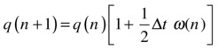
Recall that, in this equation, 1 represents the identity quaternion with a scalar component of 1 and vector components of 0; similarly, ω is the quaternion form of the angular velocity, with a scalar component equal to 0 and a vector component equal to the angular velocity vector. The third line of code in moveObject() employs the multiply() method of Quaternion to multiply and update the object’s orientation quaternion (obj.quaternion, q in the previous equation) by p. The last line normalizes the object’s orientation quaternion to avoid distortions due to numerical rounding errors.
Run the code and you’ll find that the cube behaves perfectly, rotating about the diagonal axis. Experiment by changing the value of the applied torque tqMax to make it rotate about any arbitrary axis.
Summary
Well done for making it this far into the book! You now know how to create physics simulations in 3D—in principle there is nothing stopping you from converting any of the 2D examples in the book to 3D. In the final chapter you will apply what you have learned here to create two 3D simulations—a flight simulator and a solar system simulation.