![]()
The previous two chapters covered a great deal of background material about JavaScript coding and math tools. This chapter will provide a gentle overview of basic physics to establish the final set of key concepts you’ll need to get started with physics-based programming. Along the way, we will illustrate some of these concepts using JavaScript examples and will build useful physics objects that will be used throughout the book.
Topics covered in this chapter include the following:
- General physics concepts and notation: Physics deals with measurable quantities. This brief section reviews some basic facts about the nature of physical quantities and their units, and explains the use of scientific notation for expressing the values of physical quantities.
- Things—particles and other objects in physics: Things in physics are modeled using idealized concepts such as particles. We build a JavaScript Particle object that implements appropriate particle properties and methods, and extend it to create a visible Ball object.
- Describing motion—kinematics: This section explains the concepts and methods needed to describe and analyze motion. It contains some essential definitions and formulas that any prospective physics programmer must know.
- Predicting motion—forces and dynamics: To predict motion, you need to understand what causes it: force. Dynamics is the study of force and motion. By specifying the forces acting on an object, you can compute its motion.
- Energy concepts: Energy is a powerful concept in physics and enables us to solve some otherwise tricky problems in a simple way.
General physics concepts and notation
This short section reviews some general concepts and establishes some essential terminology and notation that apply across all of physics.
In physics, when you talk about length or mass or energy, you want to be as precise as possible. Ideally, you want to be able to measure or calculate the things that you talk about. For example, the size of an object is not just a quality; it’s a quantity. Physical quantities are measurable properties. They can be given a numerical value, or magnitude.
There is something else that a physical quantity must have: a unit. For example, we don’t just say that the length of a particular table is 2; we say (in most of the world) it is 2 meters. Meter (m) is the unit. Why do we need a unit? A unit does two things. First, it tells us what kind of thing we are talking about. Meter tells us we are dealing with a length, not a temperature or something else. Second, the unit establishes a reference against which we are comparing the magnitude of the quantity. When we say that a table’s length is 2 m, what we are really saying is that the length is twice as long as that of a reference that we call the meter. All measurements are only meaningful against some reference that we compare with.
As you might imagine, there are different choices of units. For example, to measure lengths or distances, you can use meters or feet. The usual unit of length in scientific literature is the meter (m) and its subdivisions and multiples, such as centimeter (cm) and kilometer (km). The key thing is to use consistent units, not mix different types of units. Otherwise, we can use any system of units that is appropriate. For example, in computer graphics and animation work, we usually measure distances in pixels.
In the previous chapter, you came across scalars and vectors. Just to recap briefly, a vector is a mathematical object that has a magnitude and a direction, whereas a scalar is one that only has a magnitude. Physical quantities can be scalar quantities or vector quantities. An example of a vector quantity, referred to in the preceding chapter, is displacement. You’ll come across more examples later in this chapter.
You frequently encounter very large as well as very small numbers in physics. For example, the speed of light is approximately 300 000 000 m/s. Instead of writing all these zeros, we usually write this as 3 × 10⁸ m/s. The 108 (“ten to the power of 8”) is 1 followed by 8 zeros, which equates to 100 million. This is known as scientific notation. The idea is to write large or small numbers in this form, where A is greater or equal to 1 but less than 10, and B is a positive or negative integer:
![]()
As shown in the example, if B is positive, 10B is 1 followed by B zeros. What if B is a negative integer? In that case, we place the 1 in the Bth position after the decimal place, with zeros before it: for instance, 10-4 is the same as 0.0001.
As an example, the mass of an electron (the tiny particle that circles the center of atoms) is approximately 9.1 × 10⁻³¹ kg.
In JavaScript, you write this as 9.1e-31 and the velocity of light as 3e8. The “e” here must not be confused with the number e introduced in the previous chapter, which is Math.E in JavaScript. Here, e is used to denote the power of 10 by which we multiply the number preceding it.
Things: particles and other objects in physics
To describe and model the real world, physics has to have some representation of physical things. The theories of physics are conceptual and mathematical models of reality. They consist of concepts that are idealizations from the things that exist in real life. One such idealization is the concept of a particle. Although we’ll focus exclusively on particles in this section, to put them in context, here is a list of the variety of “things” you’ll come across in this book:
- Particles: Starting from this section, much of this book will deal with particles. We say more about particles shortly, but in a nutshell they can be thought of as indivisible units that exist at discrete points in space. Therefore, they are distinguished from more complex objects that can be extended or can consist of multiple parts. Particles move in a simple way: they can basically just change their position. This is also known as translation.
- Rigid bodies: A rigid body is an extended object whose size and shape cannot be changed easily, such as a table or car. Rigid bodies can move by translation like particles, but in addition they can undergo rotation. Rigid body motion will be covered in Chapter 13.
- Deformable bodies: Like rigid bodies, deformable bodies can translate and rotate, but in addition their shape and/or size can also change. Examples include a rubber ball, a rag doll, or a piece of cloth. An approach to model deformable bodies will be discussed in Chapter 13.
- Fluids:Fluids differ from the objects described previously in that they have no well-defined size or shape, but have the ability to flow from one part of space to another. Because any part of a fluid can move, it is much more difficult to simulate fluid motion accurately. But sometimes it is possible to “cheat” by modeling fluids using particles. This is the approach we take in Chapter 12 to create some interesting fluid visual effects.
- Fields: Fields are more abstract entities. In a broad sense, a field is some physical quantity that exists continuously over space. For example, we will explore the concept of a force field in Chapter 10.
What is a particle?
Because we are going to do lots of things with particles, let’s discuss them a bit more. What are particles? Probably the first things that might come to mind are tiny entities such as electrons. In physics these are called fundamental or elementary particles. That’s not necessarily what we are talking about here.
The sense in which we are going to use the word particle is as a mathematical idealization for any physical object whose inner structure or composition is not important for whatever problem we are considering. This might include atoms, or billiard balls, or even stars in a galaxy! In that sense, a particle is basically just a set of properties that characterize the object as an individual thing.
Let’s be more precise about what we mean by the last statement in the preceding section. What properties are we talking about? A particle has the following properties:
- Position: A particle has to be somewhere! That means it must have coordinates x and y (and z in 3D).
- Velocity: Particles move, so they have a velocity. We define velocity formally in the next section; for now just note that it is a vector with components, just like position.
- Mass: As a physical thing, a particle must also have mass.
- Charge: Some elementary particles, such as electrons, also have a property called an electric charge, which makes them experience an interesting type of force known as the electromagnetic force. Because we’ll play with that force in this book, we want to give our particles a charge property, too.
- Others (spin, lifetime, and so on): There are other properties we could include, taking inspiration from elementary particles in physics. But for now, we’ll stick with the properties listed here.
This background gives us enough ingredients to start building some JavaScript objects to represent particles and their behaviors, although some of the particle properties and motion concepts introduced as we do so will be covered in greater depth only as we progress through the chapter.
To start with, we will create a Particle object that implements the particle properties just described. We will then create a Ball object that extends Particle, drawing graphics so that Ball instances can be seen, while behaving as particles. Finally, we will show how to make particles move.
We need to create object properties based on the physical properties such as mass, charge, position, and velocity described in the preceding section. We should be able to read as well as modify these properties. Table 4-1 shows the properties we want to create.
Table 4-1. Properties of the Particle object
Property |
Type |
Possible Values and Meaning |
|---|---|---|
mass |
Number |
Any positive value (default 1) |
charge |
Number |
Any value: positive, negative or zero (default) |
x |
Number |
Any value; x-component of position |
y |
Number |
Any value; y-component of position |
vx |
Number |
Any value (default 0); x-component of velocity |
vy |
Number |
Any value (default 0); y-component of velocity |
pos2D |
Vector2D |
Any Vector2D value; 2D position vector |
velo2D |
Vector2D |
Any Vector2D value; 2D velocity vector |
The choice of some of these properties and their possible values requires some explanation. It is clear that mass cannot be negative or zero because every particle has mass. As you will see in Chapter 10, charge can be positive, negative, or zero. A particle with a charge of zero would behave as if it had no charge at all.
Having extolled the virtues of vectors in the previous chapter, we’d be hypocrites not to use them. Therefore, we create position and velocity vectors pos2D and velo2D as Vector2D objects from their respective components.
The implementation of these properties proceeds as follows. To begin with, we define the Particle mass, charge, x, y, vx and vy properties in its constructor:
function Particle(mass,charge){
     if(typeof(mass)==='undefined') mass = 1;
     if(typeof(charge)==='undefined') charge = 0;
     this.mass = mass;
     this.charge = charge;
     this.x = 0;
     this.y = 0;
     this.vx = 0;
     this.vy = 0;
}
We want to be able to set the mass and charge of our particles when we create them, so it makes sense to use a constructor and feed those as parameters in the constructor. Note that the values of mass and charge of a Particle instance default to 1 and 0 respectively, while the position and velocity components are all initially assigned the value of 0.
The pos2D and velo2D properties are added to the Particle prototype via getters and setters:
Particle.prototype = {
     get pos2D (){
          return new Vector2D(this.x,this.y);
     },
     set pos2D (pos){
          this.x = pos.x;
          this.y = pos.y;
     },
     get velo2D (){
          return new Vector2D(this.vx,this.vy);
     },
     set velo2D (velo){
          this.vx = velo.x;
          this.vy = velo.y;
     }
};
(Note that you may get an error with the use of these getters/setters if you use Internet Explorer, particularly IE8 or earlier.) Through these accessors, you can get or set the pos2D property of a Particle instance called particle simply by typing particle.pos2D, and similarly for the velo2D property. Naturally, you can read or assign the position coordinates of a Particle instance either using the pos2D vector of its components x and y, and similarly for velo2D. That’s all there is to the Particle object.
The file particle-example.js contains examples of the usage of the Particle object. You’ll need to launch the JavaScript console to see output from the code.
To simplify code for updating a particle’s pos2D or velo2D value, we added a couple of methods, multiply(k) and addScaled(vec, k), to the Vector2D object (where vec is a Vector2D and k is a Number). The vec1.multiply(k) method multiplies vector vec1 by the scalar k, and vec1.addScaled(vec, k) adds k times vec to vec1.
For example, to update the position of a Particle instance called particle, write this:
particle.pos2D = particle.pos2D.add(particle.velo2D.multiply(dt));
Or do this, which involves a single method call addScaled() rather than the two method calls multiply() and add():
particle.pos2D = particle.pos2D.addScaled(particle.velo2D, dt);
These are equivalent to the component form:
particle.x += particle.vx * dt;
particle.y += particle.vy * dt;
Extending the Particle object
What we’ve done in the preceding section is great stuff, but you haven’t seen any particles yet. That’s because our particles are currently invisible. The Particle object has deliberately been kept to a minimum level of complexity. It’s time now to extend it and include something that we can see. To do this, we’ll reinvent the Ball object by making some modifications to the old version that we used in previous chapters.
The Ball object
Instead of starting with the existing Ball object from previous chapters, it is easier to start with the Particle object and add some extra properties and methods to turn it into something visible. First we add a radius and a color property similar to the Ball object in Chapter 3. Then we introduce an additional property gradient, a Boolean, which specifies whether the Ball object is to be drawn with a gradient or not. Finally, we add the draw() method to Ball’s prototype, augmented to include options to draw the ball with or without a gradient. The full code for the Ball object then looks like this:
function Ball(radius,color,mass,charge,gradient){
     if(typeof(radius)==='undefined') radius = 20;
     if(typeof(color)==='undefined') color = '#0000ff';
     if(typeof(mass)==='undefined') mass = 1;
     if(typeof(charge)==='undefined') charge = 0;
     if(typeof(gradient)==='undefined') gradient = false;
     this.radius = radius;
     this.color = color;
     this.mass = mass;
     this.charge = charge;
     this.gradient = gradient;
     this.x = 0;
     this.y = 0;
     this.vx = 0;
     this.vy = 0;
}

Ball.prototype = {
     get pos2D (){
          return new Vector2D(this.x,this.y);
     },
     set pos2D (pos){
          this.x = pos.x;
          this.y = pos.y;
     },
     get velo2D (){
          return new Vector2D(this.vx,this.vy);
     },
     set velo2D (velo){
          this.vx = velo.x;
          this.vy = velo.y;
     },
     draw: function (context) {
          if (this.gradient){
               grad = context.createRadialGradient(this.x,this.y,0,this.x,this.y,this.radius);
               grad.addColorStop(0,'#ffffff'),
               grad.addColorStop(1,this.color);
               context.fillStyle = grad;
          }else{
               context.fillStyle = this.color;
          }
          context.beginPath();
          context.arc(this.x, this.y, this.radius, 0, 2*Math.PI, true);
          context.closePath();
          context.fill();
     }
};
As you can see, the constructor takes five optional arguments: radius, color, mass, charge, and gradient, with default values of 20, ‘#0000ff’, 1, 0, and false, respectively. The Boolean gradient option determines whether the ball is drawn with a gradient fill or a simple fill. The actual drawing takes place in the draw() method, as before.
Here we have created the Ball object from scratch by simply copying the properties and methods of Particle. A smarter method is to emulate classical inheritance using the Object.create() method to create the Ball object with the Particle prototype:
Ball.prototype = Object.create(Particle.prototype);
Ball.prototype.constructor = Ball;
The Ball object can then be augmented with the additional draw() method thus:
Ball.prototype.draw = function (context) {
     //code as before
}
We demonstrate this method of creating the Ball object in the file ball2.js. To use it, simply include the ball2.js file instead of ball.js in the relevant HTML file. Remember to also include the particle.js file. Whether you use ball.js or ball2.js in future examples is purely a matter of personal preference and will not affect the results in any way.
Using the Ball object
Using the Ball object is quite straightforward. This code snippet creates a ball object, initializes its position, and draws it:
var ball = new Ball(20,'#ff0000',1,0,true);
ball.pos2D = new Vector2D(150,50);
ball.draw(context);
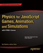
This piece of code produces a bunch of balls of random size and location, and puts them in an array so that they can be referenced in later code (see Figure 4-1):
var balls = new Array();
var numBalls = 10;
for (var i=1; i<=numBalls; i++){
     var ball;
     var radius = (Math.random()+0.5)*20;
     var color = '#0000ff';
     ball = new Ball(radius,color,1,0,true);
     ball.pos2D = new Vector2D(Math.random()*canvas.width,Math.random()*canvas.height);
     ball.draw(context);
     balls.push(ball);
}
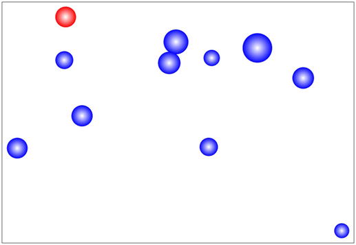
Figure 4-1. A random bunch of Ball objects
The code for these examples is in ball-test.js. To run this code, the ball-test.html file makes use of the ball.js file, whereas ball-particle-inheritance-test.html uses ball2.js (see the previous section).
Moving particles
The Ball instances depicted in Figure 4-1 look cool, but they’re just sitting there and not doing much. We need to get them moving. To make Particle (and Ball) instances move is not difficult in principle: we just need to set up an animation loop and update the particle’s position and redraw it every timestep. To do this, we will use an animation loop based on the requestAnimationFrame() method, together with the Date.getTime() method to compute time intervals accurately. We suggest that you take a look at the last example in Chapter 2, getTime-example.js, to refresh your memory about the basic logic and code structure. The example code in ball-move.js builds upon the code in getTime-example.js (Chapter 2) and is shown here in its entirety:
var canvas = document.getElementById('canvas'),
var context = canvas.getContext('2d'),

var ball;
var t;
var t0;
var dt;
var animId;
var animTime = 5; // duration of animation

window.onload = init;

function init() {
     ball = new Ball(20,'#ff0000',1,0,true);
     ball.pos2D = new Vector2D(150,50);
     ball.velo2D=new Vector2D(30,20);
     ball.draw(context);
     t0 = new Date().getTime();
     t = 0;
     animFrame();
};

function animFrame(){
     animId = requestAnimationFrame(animFrame,canvas);
     onTimer();
}
function onTimer(){
     var t1 = new Date().getTime();
     dt = 0.001*(t1-t0);
     t0 = t1;
     t += dt;
     if (t < animTime){
          move();
     }else{
          stop();
     }
}
function move(){
     ball.pos2D = ball.pos2D.addScaled(ball.velo2D,dt);
     context.clearRect(0, 0, canvas.width, canvas.height);
     ball.draw(context);
}
function stop(){
     cancelAnimationFrame(animId);
}
Much of the code deals with setting up the time-keeping, as described in Chapter 2, and should therefore be familiar. The init() function creates a Ball instance, initializes its position and velocity, and draws it on the canvas. It then initializes the time variables and calls the animFrame() function, which sets up the animation loop. The onTimer() function, which fires at every timestep, computes the time interval elapsed (in seconds) since the first call, dt, and then updates the time duration from the beginning of the simulation, t (in seconds). The latter is computed by summing all the elapsed time intervals dt up to the current one. The onTimer() function also contains an if loop that then calls the move() function if the total elapsed time of the simulation is less than a specified duration animTime, and calls a stop() function otherwise, which terminates the animation loop. The move() function updates the ball’s position vector based on its velocity vector, erases everything on the canvas, and redraws the ball object. Open the file ball-move.html in a web browser and you will see a ball moving at a constant velocity across the canvas.
The basic setup for the time-keeping in this code will be used over and over again in future examples. The next example, balls-move.js, extends the code to make several balls move at the same time. The only substantial changes take place in the init() and move() methods:
function init() {
     balls = new Array();
     for (var i=0; i<numBalls; i++){
          var radius = (Math.random()+0.5)*20;
          var ball = new Ball(radius,'#0000ff',1,0,true);
          ball.pos2D = new Vector2D(canvas.width/2,canvas.height/2);
          ball.velo2D = new Vector2D((Math.random()-0.5)*20,(Math.random()-0.5)*20);
          ball.draw(context);
          balls.push(ball);
     }
     t0 = new Date().getTime();
     t = 0;
     animFrame();
};
In init(), a number of balls are now created and their position and velocity are initialized. They are then placed into an array named balls, as in the example in the previous section. This time, the array is actually used in the move() function:
function move(){
     context.clearRect(0, 0, canvas.width, canvas.height);
     for (var i=0; i<numBalls; i++){
          var ball = balls[i];
          ball.pos2D = ball.pos2D.addScaled(ball.velo2D,dt);
          ball.draw(context);
     }
}
As you can see, we loop over all the elements of balls to update the position of each ball and redraw it on the canvas element. Run the code by opening the file balls-move.html in a browser and you’ll see balls of different sizes moving out from the same initial location.
In all these examples, the balls move at a constant velocity. The really interesting situation is when the velocity changes with time; we’ll do that soon in this chapter. But first we need to introduce some motion concepts.
In this section, we will start to describe motion more formally using precise concepts, equations, and graphs. The description of motion is called kinematics. In kinematics, we are not concerned with what causes motion, but only with how to describe it. The next section, “Predicting motion: forces and dynamics,” will look at the cause of motion: force.
Concepts: displacement, velocity, speed, acceleration
Up to now, we’ve talked about things like velocity and acceleration rather loosely. It’s time now to say precisely what we mean by these quantities.
Here are the main concepts that require definition in kinematics:
- Displacement
- Velocity (and the associated concept of speed)
- Acceleration
These physical quantities rest upon more fundamental concepts—position, distance, and time—that are taken as self-evident and do not require definition. For vector quantities, there is a fourth basic concept: angle, which defines a direction in space.
Displacement is a vector quantity associated with the motion of an object. To be more precise, it’s the vector connecting the initial position with the final position of the object. Remember the example of Bug from Chapter 3? Bug moves a distance of 10 units along the y-axis from the origin—that’s a displacement. From there, it then undergoes another displacement of 10 units to the right (in the positive x direction).
In this example, the net or resultant displacement of Bug is then ![]() , or approximately 14.1 units at an angle of 45 degrees. But the net distance it moves is, of course, 20 units. This example illustrates the difference between displacement and distance. In general, an object might move along any complicated trajectory: the distance moved would then be the length along the trajectory, whereas the displacement would always be the vector joining the initial position to the final position of the object (see Figure 4-2).
, or approximately 14.1 units at an angle of 45 degrees. But the net distance it moves is, of course, 20 units. This example illustrates the difference between displacement and distance. In general, an object might move along any complicated trajectory: the distance moved would then be the length along the trajectory, whereas the displacement would always be the vector joining the initial position to the final position of the object (see Figure 4-2).
Figure 4-2. Displacement vector (arrow) contrasted with distance along trajectory
Displacement is usually denoted by the symbol s or x, and its magnitude as s or x. The usual unit of displacement (and distance) is the meter and its multiples (for example, km) and fractions (cm, mm, and so on). On canvas, where you’ve got a stage on a computer screen rather than real space, you’ll think of distance and displacement in terms of pixels, which we’ll often abbreviate as px.
Velocity is defined as the rate of change of displacement with time. It tells you how quickly something is moving, but also in what direction it is moving. Hence, velocity is a vector quantity.
The usual symbol for velocity is u or v; for its magnitude, u or v.
Remember what rate of change means in calculus? It’s the gradient function, or derivative. Therefore, velocity is the derivative of displacement with time. In calculus notation we write this as

Again, this derivative is the limit of the ratio Δs/Δt as the time interval Δt (and therefore also the displacement change Δs) becomes small. So, for finite intervals, we can write

This gives us the average velocity over the time interval Δt, whereas v = ds/dt gives us the instantaneous velocity at a given time. In the special case where velocity is constant, the average velocity is equal to the instantaneous velocity at any time.
As mentioned before, the usual unit for velocity in physics is meters per second (m/s), although km/hr and miles/hr are commonly used in everyday life. In a canvas context, the measure of time is still the second, but the measure of distance is the pixel. So, you’ll usually think of velocity in terms of pixels per second (px/s).
In computer code, we are always dealing with discrete intervals, so we are really dealing with average velocities. But if we use a small enough time interval, the average is close to the instantaneous value. One can rearrange the preceding equation to give Δs in terms of v and Δt:
![]()
This equation tells us that the displacement increment is given as the product of velocity and the time interval. This is exactly what we do in the move() method in the ball-move.js example:
ball.pos2D = ball.pos2D.addScaled(ball.velo2D,dt);
You might also recognize this as being equivalent to integrating in time using the forward scheme (refer to Chapter 3). That makes perfect sense—because velocity is the derivative of displacement with time, displacement is the integral of velocity with time. We’ll use this integration scheme, specifically known as an Euler scheme, until we get to Part IV of the book.
Speed is the scalar version of velocity; it has no direction. Speed is defined as the rate of change of distance with time, or, in other words, as distance moved per unit of time. The unit of speed is the same as that of velocity.
The average speed of an object is the total distance travelled divided by the total time taken:
In this book, most of the time we’ll be dealing with velocity and velocity components rather than speed.
Acceleration is defined as the rate of change of velocity with time. It tells you how fast an object’s velocity is changing. If you’re driving a car at a constant velocity of 20 m/s (approximately 45 miles/hr) in a straight line, you’re not accelerating—the acceleration is zero. But if you apply the accelerator and increase the car’s speed from 20 m/s to 30 m/s in 10 seconds, the average acceleration is (30 – 20)/10 m/s per second, or 1 m/s2. This means that the velocity increases by 1 m/s in each second. Acceleration can also be negative; in that case, the velocity magnitude decreases.
The calculus definition of acceleration is

and the discrete version is

These equations are similar to those for velocity, with displacement replaced by velocity. Like the corresponding equations for velocity, a = Δv/Δt gives us the average acceleration over the time interval Δt, whereas a = dv/dt gives us the instantaneous acceleration at a given time.
![]() Note In the special case where acceleration is constant, the average acceleration is equal to the instantaneous acceleration. We’ll illustrate this fact in the next section.
Note In the special case where acceleration is constant, the average acceleration is equal to the instantaneous acceleration. We’ll illustrate this fact in the next section.
Reversing the previous equation gives this:
![]()
Interpreted as a discrete equation, this gives us an integration scheme for updating velocity given the acceleration. This is how you would code it in JavaScript using Vector2D:
particle.velo2D = particle.velo2D.add(acc.multiply(dt));
or
particle.velo2D = particle.velo2D.addScaled(acc, dt);
Here acc is a variable representing acceleration. It is a Vector2D object. Suppose we use a fixed value:
var acc:Vector2D = new Vector2D(0,10);
This will make our particles accelerate downward at a rate of 10 px/s2, simulating the effect of gravity.
Because acceleration is the rate of change of velocity, it is nonzero if the direction of motion changes, even if the speed is constant. A common example is that of an object moving at constant speed in a circle. Because the object’s direction of motion changes, its velocity changes. Therefore, its acceleration is not zero. We’ll look at this situation in detail in Chapter 9.
Combining vector quantities
Because displacement, velocity, and acceleration are vector quantities, it goes without saying that they must be combined (added or subtracted) using vector methods. You saw an example of how this is done in the previous chapter, so we won’t repeat it here.
Why would you want to combine these quantities? You’ll frequently want to add displacements and velocities to calculate their total (also known as their resultant). Again, you saw an example of resultant displacement in Chapter 3. An example of a situation in which you would want to add velocities is that of a boat on a flowing river. The resultant velocity of the boat is then given by the vector sum of its velocity in the water with the velocity of the water current (see Figure 4-3).
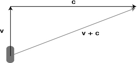
Figure 4-3. Resultant velocity
You’ll need to use vector subtraction when calculating relative velocities. Suppose you have spaceship A chasing another spaceship B, moving at different velocities a and b in space (see Figure 4-4). What is the velocity of B relative to A? That’s the velocity of B from the point of view of A. In other words, it’s the velocity of B in a frame of reference in which A is not moving (we say it’s at rest). A little quiet thinking should convince you that it’s given by the velocity of B minus that of A, in a vector sense: b – a. Figure 4-4 shows you what b – a means geometrically: it’s the same as b + (–a), and because (–a) points opposite to a with the same magnitude, we end up with b – a pointing in the direction shown. This is the velocity of B as seen by A from its point of view.
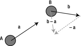
Figure 4-4. Relative velocity
Describing motion using graphs
The motion of an object can be represented graphically in different ways. For a particle moving in two dimensions, you can plot its y-coordinate against its x-coordinate at different times. The resulting graph would, of course, just give you the trajectory of the particle.
You can also plot the components of displacement, velocity, or acceleration against time. These graphs can tell us useful information about how the particle moves.
You will soon see examples in which we make use of the Graph object that we introduced in the previous chapter to create such plots.
Equations of motion for uniform acceleration
For the special case of motion under constant acceleration (also known as uniform motion), it is possible, starting only from the definitions of velocity and acceleration, to arrive at a very useful set of equations. These equations of motion can be used to analyze problems in which the acceleration is constant, including the motion of bodies falling under gravity and the motion of projectiles.
We could just state the equations of motion and ask you to accept them. But you might understand them better if you see where they come from. And it’s not really difficult; you just need to do a tiny amount of algebra. The starting point is the definition of average acceleration:

If the acceleration is constant, aav is also equal to the instantaneous acceleration a at any time t.
Let’s now establish our initial conditions by saying that at time t = 0 (initially), s = 0 (zero initial displacement), and v = u (the initial velocity is denoted by u).
Therefore at time t, we have Δv = v – u, and Δt = t – 0 = t, so that

It is now easy to change the subject of this formula to get this:
![]()
This formula gives us the velocity v at any time t, given the initial velocity u and the (constant) acceleration a.
It would be nice to have a similar equation for displacement too. Can it be done? Yes, you just need to apply the same trick, this time starting from the definition of average velocity:

Now we have Δs = s – 0 = s, and Δt = t – 0 = t, which gives

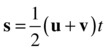
Because the velocity increases linearly, the average velocity vav is just ![]() (u + v), the average of the initial and final velocities. Substituting into the preceding equation gives this:
(u + v), the average of the initial and final velocities. Substituting into the preceding equation gives this:
Now you can use the formula already derived (v = u + a t) to substitute for v. Do this and simplify, and you should get this:
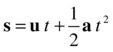
Now sit down and admire this remarkable result of your hard work. What you have here is a formula that tells you the displacement s of a particle at any time t, in terms of the initial velocity u of the particle and the (constant) acceleration a.
This will equal the position vector of the particle at time t if it starts out at the origin at time t = 0. In general, if the particle starts out at location pos0 = (x0, y0, z0) at time t = 0, its position vector pos = (x, y, z) at time t will be given by the following, in pseudocode:
pos = u * t + 0.5 * a * t * t + pos0
This gives you the position of the particle as an exact analytical equation. There is no need to use numerical integration in this case.
You can code up this solution directly in vector form (as we do), or split it into components if you prefer. In pseudocode, you get this in 3D (in 2D just ignore the z component):
x = ux * t + 0.5 * ax * t * t + x0
y = uy * t + 0.5 * ay * t * t + y0
z = uz * t + 0.5 * az * t * t + z0
Before we leave this section, you should know that there is a third formula that sometimes proves useful. The two formulas derived previously (v = u + at, and s = u t + ![]() a t2) give you the velocity v and the displacement s, each as a function of time t. If you eliminate the time t between these two equations, you can get an equation for v and s in terms of each other:
a t2) give you the velocity v and the displacement s, each as a function of time t. If you eliminate the time t between these two equations, you can get an equation for v and s in terms of each other:
![]()
Note that this one is a scalar equation, not a vector equation.
![]() Caution As mentioned earlier, the equations of motion derived in this section are valid only for constant acceleration. If the acceleration changes with time, they will give the wrong answer.
Caution As mentioned earlier, the equations of motion derived in this section are valid only for constant acceleration. If the acceleration changes with time, they will give the wrong answer.
Example: Applying the equations to projectile motion
It’s time for an example. Let’s apply the preceding equations to model the motion of a projectile such as a cannonball. To do this, we’ll neglect all other forces except gravity. In that case, the force on the projectile at any time during its flight is constant. This will give it a constant acceleration (you’ll understand fully why in the next chapter).
We do not model the explosive force that shoots the cannonball in the first place. That force is very brief, and its effect is to impart an initial velocity u to the cannonball.
In this special case, the equations for the position of the projectile in component form reduce to this, in pseudocode:
x = ux * t + x0
y = uy * t + 0.5 * g * t * t + y0
z = uz * t  + z0
Because the acceleration due to gravity points vertically downward, its x and z components ax and az are zero, and ay = g. If you use vectors, you simply need to specify the acceleration vector as (0, g, 0) in 3D and (0, g) in 2D in the equation pos = u * t+ 0.5 * a * t * t + pos0.
Let’s use these formulas to code a simple projectile simulation. The code is in projectile-test.js and is reproduced here:
var canvas = document.getElementById('canvas'),
var context = canvas.getContext('2d'),

var ball1;
var ball2;
var t;
var t0;
var dt;
var animId;
var pos0 = new Vector2D(100,350);
var velo0 = new Vector2D(20,-80);
var acc = new Vector2D(0,10); // acceleration due to gravity
var animTime = 16;

window.onload = init;

function init() {
     ball1 = new Ball(15,'#000000',1,0,true);
     ball1.pos2D = pos0;
     ball1.velo2D = velo0;
     ball2 = new Ball(15,'#aaaaaa',1,0,true);
     ball2.pos2D = pos0;
     ball2.velo2D = velo0;
     ball1.draw(context);
     ball2.draw(context);
     t0 = new Date().getTime();
     t = 0;
     animFrame();
};

function animFrame(){
     animId = requestAnimationFrame(animFrame,canvas);
     onTimer();
}
function onTimer(){
     var t1 = new Date().getTime();
     dt = 0.001*(t1-t0);
     t0 = t1;
     if (dt>0.2) {dt=0;}; // fix for bug if user switches tabs
     t += dt;
     if (t < animTime){
          move();
     }
}
function move(){
     // numerical solution - Euler scheme
     ball1.pos2D = ball1.pos2D.addScaled(ball1.velo2D,dt);
     ball1.velo2D = ball1.velo2D.addScaled(acc,dt);
     // analytical solution
     ball2.pos2D = pos0.addScaled(velo0,t).addScaled(acc,0.5*t*t);
     ball2.velo2D = velo0.addScaled(acc,t);
     // display
     context.clearRect(0, 0, canvas.width, canvas.height);
     ball1.draw(context);
     ball2.draw(context);
}
In the init() function, the code creates two balls (one gray and one black), which are initially positioned at the same location (100, 350), have the same initial velocity (20, –80), and are subjected to the same downward acceleration (0, 10) to simulate gravity. In the move() function, the positions and velocity of these two balls are updated differently. For the first ball, we implement the Euler integration scheme (as discussed in the section on velocity) for updating the velocity by adding the acceleration times the current time interval dt. Similarly for the position of the ball. For the second ball, we assign a new current position based on the exact analytical formula pos = u * t+ 0.5 * a * t * t + pos0. No numerical approximation is then involved.
Before you run the code, note the following additional line of code in onTimer():
if (dt>0.2) {dt=0;};
This is a fix for a bug that arises if the user switches browser tabs and then returns. When this happens, requestAnimationFrame() ceases to be active until the user returns to the current tab, so that the animation “freezes” on the current frame. However, when the user returns the elapsed time dt is still computed as the difference between the last call to getTime()and the current time, resulting in an artificially large value of dt in that frame. The code in the move() function then updates the particle’s position using the same velocity over the large time interval dt. This would have been fine if the velocity were constant, as in the ball-move.js example we saw earlier in this chapter. But in general, as in the present example, the velocity would in reality be changing due to acceleration. The artificially large value of dt would then result in unphysical deviations or “jumps” in the position of the particle from where it should be. The previous line of code fixes this problem simply by setting the value of dt to 0 if its value happens to be larger than a threshold value of 0.2 seconds. The value of 0.2 is essentially arbitrary, and you can use any value you like as long as it is much larger than the typical value of dt when the animation is running normally (here that would be of order 20 milliseconds, which is ten times less than 0.2 seconds) and much smaller than the time it takes to switch to a new tab and back.
If you run the code, you’ll see both balls start off together and move in a parabolic path as projectiles are supposed to do. As the simulation progresses, you’ll see them begin to separate slightly, as pictured in Figure 4-5, because of numerical errors due to the Euler scheme.
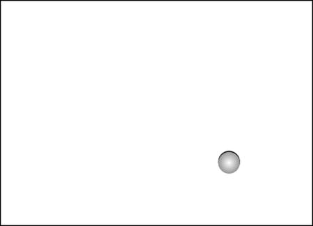
Figure 4-5. Simulating the motion of a projectile with both numerical and analytical solutions
The gray ball is exactly where it should be because it follows the exact analytical solution of the equation of motion. Now you probably won’t normally care about the difference. But if you’re building an accurate simulation of projectiles or a game of billiards, you would. The difference in position shown in Figure 4-5 is after only 16 seconds of run time. If you were to run this for a few minutes and include bouncing or collisions with other particles, your particle would soon be in places it shouldn’t be.
So, what can be done about this if your simulation or game requires high accuracy? If your simulation is simple enough for an analytical solution to exist (as in the present example), using that solution would solve the problem. However, in the vast majority of scenarios, analytical solutions do not exist. In those cases, you need to use a more accurate integration scheme than the Euler scheme.
Chapter 14, in Part IV of the book, covers some more accurate integration schemes. But before we get there, we will use the Euler scheme in most of the examples because Euler is the simplest and quickest scheme, and our main aim in much of the book prior to Part IV is to demonstrate physics effects without necessarily worrying too much about absolute accuracy. As we go along, we will point out examples in which the lack of accuracy may be especially important, although we will defer any solutions to Chapter 14.
The choice of integration scheme is not the only consideration if you are worried about numerical accuracy. Errors can also arise due to the algorithms for dealing with sudden changes such as bouncing and collisions. We’ll discuss these other sources of error and how they can be dealt with later in the book.
More motion-related concepts: inertia, mass, and momentum
So far, we’ve been limited to a few motion concepts, and the progress we can make just with those is rather restricted. The greatest power comes with the notion of forces and how they affect motion. We’ll introduce that approach in a conceptual way in the next section and then develop it fully in the next chapter.
Before we do so, we need to introduce two new concepts that act as a connection between motion and the forces that produce them: mass and momentum.
Let’s start with mass. In physics, mass has a very specific meaning: it is a measure of inertia. Inertia (literally “laziness”) is resistance to motion. The more massive an object is, the more it resists motion—it is more difficult to push a car than a bike. So we say that the mass of a car is larger than that of a bike. The usual unit of mass in physics is the kilogram (kg). The usual symbol for mass is m.
In physics, the mass of an object is not the same as its weight. Weight is actually a force, the force of gravity that the Earth exerts on it. Mass is a scalar; weight is a vector. We’ll come back to this in the next section.
The momentum of an object, denoted usually by the symbol p, with magnitude p, is defined as the product of its mass and its velocity. It is a vector quantity.
![]()
Because it is equal to a scalar (mass) times velocity, it has the same direction as that of the velocity vector.
Informally, momentum is a measure of the “quantity of motion” that a body possesses—for the same velocity, a car has “more motion” than a bike because it is more difficult to stop the car. Momentum is important for two reasons: it is intimately connected with force, and there is a law known as the law of conservation of momentum that’s very useful for solving problems such as collisions between particles. We’ll take a close look at momentum and its conservation in the next chapter.
Predicting motion: forces and dynamics
In the preceding section, we could “solve” the projectile problem by obtaining a formula for the position of the projectile as a function of time. That was possible because we knew the acceleration—it was constant and was equal to g, the acceleration due to gravity.
The problem of predicting the motion of an object basically boils down to calculating the acceleration at each time a(t), whether by some analytical formula or by some numerical procedure. Once we know a, we know how to do the rest—we can integrate numerically (using the Euler or some other scheme) or use an analytical solution if one exists.
In the case of gravity near the Earth’s surface, you now know that a = g, so that’s nice and simple. But how can we calculate the acceleration of an object in general? Before we can give the answer, we need to talk a bit more about forces.
The cause of motion: forces
A force is an abstract concept in physics that denotes “something” that makes things move. To be more precise, if a bit mysterious, forces change the way things move. The meaning of this statement will be made clear in just a moment.
Intuitively, you can think of a force as some kind of push or pull. Gravity is a force; it pulls you toward the Earth. Friction is another type of force; it pushes against a moving object.
Forces can be measured and calculated. The unit of force is the newton, denoted by the symbol N.
Forces are useful because knowing the forces acting on a body allows prediction of its motion. How this is done will be explained next.
The relationship between force, mass, and acceleration
Let’s go back to the question we asked at the beginning of this section. How can we work out the acceleration of an object? The answer turns out to be surprisingly simple:
![]()
F is the total force acting on an object, m is its mass, and a is the acceleration produced by the force. That’s it. This is a remarkable formula, probably the most important in this book. It’s remarkable because it connects motion (more precisely, acceleration) with its cause (force) in probably the simplest way you can imagine.
The equation F = ma is a special case of Newton’s second law of motion. It’s the most common form of this law. In the next chapter, we’ll look at the general form of the law.
You can rewrite the formula as follows, which you can use to calculate the acceleration a given the mass m of an object and the force F acting on it:

As we discussed in Chapter 1, the motion of an object is a function of the forces acting on the object:
motion = function{forces}
Well, a = F/m is exactly what that means. That’s our function. Forces cause acceleration; they cause the velocity of an object to change. And that’s how we calculate that change in motion.
This formula is consistent with our conceptual idea of force and mass as respectively causing and resisting motion. For a given force, the acceleration produced is less for a larger mass because we’ll be dividing the force by a larger number.
The next question is this: how do we know the force F? Well, in fact, there are many different types of forces. Luckily, there are formulas for each type of force. The formulas come from physics theories or experiments. For us, it does not matter where they come from, of course. The point is that we can calculate all the forces acting on an object at any time and then add them all up to give the total or resultant force F. We then divide this total force F by the mass m of the object; that gives us the acceleration a of the object. Problem solved.
Types of forces
In Part II of the book, we’ll be looking at different types of forces in a lot of detail. Here are some quick examples.
Gravity is perhaps the most obvious example of a force. The force of gravity acting on an object is also known as its weight. The Earth (or any other planet or star) exerts a gravitational force on any object near it that is in proportion to the mass of that object. So the weight of an object of mass m is given by
![]()
where g is a vector that points vertically downwards with constant magnitude g.
Using a = F/m, this gives a = mg/m = g. In other words, the weight of an object (the force of gravity on it) produces an acceleration of g if it’s the only force acting on the object. This shows that g is actually an acceleration, known as the acceleration due to gravity. Near the Earth’s surface, it has a magnitude of approximately 9.81 m/s2. Note that the mass m of the object “drops out”—all objects fall with the same acceleration regardless of their mass or size (as long as other forces such as air resistance are negligible compared with gravity).
Another common type of force is a contact force, which is the force that an object experiences when it comes into direct physical contact with another object. This occurs, for example, when you push something, when two objects collide, or when two things are pressed together by another force (for example, a book pressing against a table because of its weight). If you are reading a physical copy of this book, lay it on the table. The reason it does not fall through the table is that the latter is exerting an upward contact force that balances the force of gravity on the book.
Another type of contact force is friction, which acts when two objects that are in contact move relative to each other. If you push the book along the table, friction is the force that resists the motion of the book. We’ll look at contact forces in Chapter 7.
There are also several examples of forces caused by fluids, such as pressure, drag (a type of frictional force), and upthrust. We’ll look at these forces in detail in Chapter 7.
Then there are electric and magnetic forces, which can also act together as an electromagnetic force. These forces are exerted and experienced by particles and objects that possess a physical property called electric charge. In fact, apart from gravity, all the everyday forces such as contact forces, fluid forces, and so on originate from the electromagnetic forces that atoms and molecules exert on each other. We’ll look at these forces in Chapter 10 and see how they can be used to produce interesting effects.
Combining forces: force diagrams and resultant force
In the equation F = ma, F is the total or resultant force. Because force is a vector quantity, the resultant force due to two or more forces must be obtained by vector addition, as described in Chapter 3.
A vector diagram that shows the forces acting on a body is called a force diagram. Force diagrams can be useful tools because they help us to work out the resultant force. The point is that it does not matter if the forces acting on a body are of different types. You can add gravity to friction and drag, for example, as long as you do so using vector addition.
As vectors, forces can be “resolved” or “decomposed” into perpendicular components, as explained in Chapter 3. Sometimes it might prove helpful to analyze a problem by resolving forces into their components and combining all the horizontal and vertical components separately.
Figure 4-6 shows an example of a force diagram. It shows the forces acting on an object sliding down an inclined plane. There are three forces acting on this object: its weight mg, which acts downward; a frictional force f exerted by the surface, which acts opposite to the direction of its motion; and a contact force R, which the surface exerts upon it, acting perpendicular to the surface. Note that you don’t care about the force that the object exerts on the surface. If you are modeling the motion of an object, you care only about the forces acting on it, not the forces exerted by it.

Figure 4-6. Force diagram for a body sliding down an inclined plane
If you were to simulate the motion of an object such as the one shown in Figure 4-6 (perhaps a car going downhill), how would you do it? As always, with a bit of common-sense logic, some physics formulas, and some code. We won’t go into detail about the physics and coding (we’ll save that for Chapter 7, when we look at friction and contact forces in detail), but here is the common-sense part. From experience, you know that the object will slide along the surface while always maintaining contact. So it makes sense to resolve the forces along the plane. Well, f is already along the plane; R is perpendicular to it and so has no component along it; the component of gravity force (weight) is mg sin 30° down the incline. Hence, the magnitude of the resultant force down the incline is given by
![]()
Of course, you’ll need to know how to calculate the frictional force f. We’ll tell you that in Chapter 7. Once you know f, you can calculate the acceleration a = F/m, as you must surely know by now.
Sometimes, with two or more forces acting on an object, it so happens that the vector sum (resultant) of the forces is zero. In that case the forces are said to be in equilibrium. In terms of the motion of the body, it’s as if no forces were acting on it.
Let’s go back once more to the equation a = F/m. The equation implies that if the resultant force F = 0, then a = 0. Therefore, if there is no resultant force acting on a body, the body does not accelerate. In other words, its velocity does not change, whatever it is. This means two things. First, if the object is not moving (if it’s at rest), it will remain at rest. But also, if the object was already moving at some velocity, it will maintain that velocity and neither accelerate nor decelerate (which is really a negative acceleration). The latter conclusion might come as a surprise to you; we’ll pick up on it again when we discuss Newton’s laws of motion in the next chapter.
Figure 4-7 shows two examples of an object in equilibrium while under the action of more than one force. In the first example, a book rests motionless on a level table, so it must experience at least two forces that add up to zero. You know that one of them must be the force of gravity, which acts downward. There is another force, a contact force R that the table exerts on the book that acts upward, opposing the force of gravity exactly.
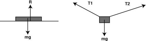
Figure 4-7. Examples of forces in equilibrium
The second, slightly more complicated example again shows an object at rest. But this time there are three forces acting on it. The object is suspended by means of two strings. So there is a tension force in each string as well as the force of gravity acting on the object. If you add up the three forces, their vector sum must be zero. And if you resolve each force into horizontal and vertical components and then add all the horizontal components together and all the vertical components together, both will add up to zero.
The example in Figure 4-8 shows the force diagram for a plane flying at constant velocity. From the previous discussion, we again deduce that the resultant force on it must be zero, no matter how many forces there are or how complicated they are. In fact there are four main forces acting on the plane: a forward thrust, an opposing drag, a downward weight, and an upward lift. Lift balances the weight of the plane, and thrust balances the drag force on the plane. It may sound a bit counterintuitive that the thrust and drag are equal. In fact, thrust must exceed drag only when the plane is accelerating, for example during take-off and ascent. But once the plane has reached a uniform velocity, thrust is needed only to overcome drag.
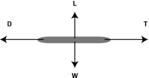
Figure 4-8. Forces on a plane moving at constant velocity are also in equilibrium
Example: Object falling under gravity and drag
All this discussion of forces might appear somewhat abstract, and you are probably eager to see how it’s all applied in practice. Although we’ll have plenty of examples in Part II, let’s look at a simple example now to whet your appetite. Don’t worry if you don’t understand everything immediately: it will all make complete sense after you’ve seen a few more examples in Part II.
In this example, a ball is dropped in a fluid such as air and, as it falls, it experiences a downward force of gravity W and an upward drag force D (see Figure 4-9). Gravity is, of course, constant and given by this:
![]()
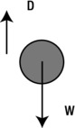
Figure 4-9. A ball falling in air, experiencing forces of gravity W and drag D
We’ll have more to say about the drag force in Chapter 7; for now we just borrow the following formula:
![]()
In other words, the drag force is proportional to the velocity of the ball through the fluid (the minus sign indicates that the drag force is opposite in direction to the velocity, and k is a constant of proportionality). Using these two formulas, we can make the following deductions. Initially, the ball is at rest, so the drag force on it is zero. As the ball falls, it accelerates under gravity, so its velocity increases, and so does the drag force D. Eventually (if the ball falls long enough without hitting the ground), the drag force will become equal to the force of gravity, so the two will balance. At that point, we’ll have equilibrium, so the acceleration will be zero, as discussed in the previous section. The ball will then continue falling at a constant velocity, known as terminal velocity. This is what we expect to happen according to physics theory, but can we reproduce it in a simulation?
To demonstrate that we indeed can simulate the ball’s motion under the action of these forces, we will animate its fall while simultaneously plotting its velocity and acceleration as time progresses. Take a look at the code in the file forces-example.js and the markup in the file forces-example.html, in which it is embedded.
First you’ll notice that we have two canvas instances in the HTML file, with IDs of canvas and canvas_bg. The canvas instance is placed exactly on top of canvas_bg and made transparent (see the style file style1.css to find out how this is done). The idea is that we will place a static Graph instance on canvas_bg, and animate the ball on canvas. Note also that we have to include the graph.js file in addition to vector2D.js and ball.js in the HTML file.
The code in forces-example.js builds upon previous examples but also adds some important new elements. The init() function looks like this:
function init() {
     ball = new Ball(15,'#000000',1,0,true);
     ball.pos2D = new Vector2D(75,20);
     ball.velo2D=new Vector2D(0,0);
     ball.draw(context);
     setupGraphs();
     t0 = new Date().getTime();
     t = 0;
     animFrame();
};
This is very familiar: what’s new here is the addition of the setupGraphs() method, which sets up a couple of Graph instances on canvas_bg on which to plot the velocity and acceleration of the ball as it falls:
function setupGraphs(){
     //graph = new Graph(context,xmin,xmax,ymin,ymax,xorig,yorig,xwidth,ywidth);
     graphAcc = new Graph(context_bg,0,30,0,10,150,250,600,200);
     graphAcc.drawgrid(5,1,5,1);
     graphAcc.drawaxes('time (s)','acceleration (px/s/s)'),
     graphVelo = new Graph(context_bg,0,30,0,25,150,550,600,200);
     graphVelo.drawgrid(5,1,5,1);
     graphVelo.drawaxes('time (s)','velocity (px/s)'),
}
The animFrame() function called in init(), which sets up the animation, is essentially the same as in the previous projectile example, but the time-stepping move() method now looks different:
function move(){
     moveObject();
     calcForce();
     updateAccel();
     updateVelo();
     plotGraphs();
}
For pedagogical reasons mainly, we’ve split the code into separate functions whose tasks should be evident from their names. First, the moveObject() method updates the ball’s position and redraws it, and it looks like this:
function moveObject(){
     ball.pos2D = ball.pos2D.addScaled(ball.velo2D,dt);
     context.clearRect(0, 0, canvas.width, canvas.height);
     ball.draw(context);
}
This does nothing new that we haven’t seen before. The significant additions are the three methods calcForce(), updateAccel(), and updateVelo(), which look like this:
function calcForce(){
     force = new Vector2D(0,ball.mass*g-k*ball.vy);
}
function updateAccel(){
     acc = force.multiply(1/ball.mass);
}
function updateVelo(){
     ball.velo2D = ball.velo2D.addScaled(acc,dt);
}
As you can see, these functions respectively compute the resultant downward force using F = mg – kv, the acceleration using a = F/m, and the new velocity using Δv = a Δt. So we subject the ball instance to the two forces of gravity and drag, calculate their resultant force, and then calculate the acceleration and velocity. The position is updated at the next timestep in the moveObject() method.
The final method, plotGraphs(), plots the vertical components of acceleration and velocity on the respective Graph instances on canvas_bg:
function plotGraphs(){
     graphAcc.plot([t], [acc.y], '#ff0000', false, true);
     graphVelo.plot([t], [ball.vy], '#ff0000', false, true);
}
Run the code, and you will see something like Figure 4-10. As the ball falls, it initially accelerates at the value of g = 10 (as set in the code) and its velocity starts to increase sharply. But then the drag force starts increasing; this reduces the resultant downward force and therefore the downward acceleration, causing the velocity to increase less rapidly. About 10 seconds into the simulation, the acceleration has fallen to zero because the drag force has now grown enough to exactly balance the downward force of gravity. From then onward, the ball’s velocity is constant at the value of 20 px/s. This is all just as described previously, so the simulation really works! In fact, the value of the terminal velocity is exactly as predicted by physics theory.

Figure 4-10. Simulating a ball falling under gravity and drag
To see this, we reason that when terminal velocity is reached:
drag = gravity,
and so
![]()
This gives v = mg/k. In our simulation, m = 1, g = 10 and k = 0.5. This gives v = 20 px/s, exactly as computed by the simulation. Not bad at all for a first example on forces, don’t you agree?
Energy concepts
We’ve talked a lot about forces, but there is another physics concept that is perhaps equally important: energy. From our point of view, the important thing is that energy concepts sometimes provide an alternative way to solve problems that can prove tricky or even impossible to solve using the approach of forces. Just as you saw with momentum, this is because there is a powerful law of conservation of energy (which we’ll talk about shortly). In fact, conservation of energy and momentum can be applied together to solve problems involving collisions, as we shall see in Chapter 5 and, in more detail, in Chapter 11.
Unlike momentum, energy is a bit trickier to define. Before we can do so, we need to introduce a closely related concept—that of work.
The notion of work in physics
We’ve often said that force causes motion, but we’ve also seen that a force can exist in equilibrium with other forces, so that motion cannot occur. To distinguish the motion-producing effect of a force from that of merely balancing another force, we introduce the concept of work.
In physics, we say that work is done by a force when it produces motion in the direction along which it acts. The amount of work done W is then defined as the product of the force magnitude F and the displacement s in the direction of the force:
![]()
That may sound a bit abstract, so let’s look at an example. Let’s say a stone is dropped from a certain height h above the ground (see Figure 4-11).

Figure 4-11. An object dropped from rest at a height h above the ground
Then the weight of the stone (the force of gravity on it) does work by displacing it downward. According to the preceding definition, the amount of work done in falling a distance h to the ground is therefore given by the following formula, because here F = mg and s = h:
![]()
Because work is the product of a force and a distance (and recalling that the unit of force is the newton, N), its unit is Nm (newton times meter). This unit also has a special name, the joule (J). So, J = Nm. Work is a scalar quantity.
What if the displacement is not in the same direction as the force? For example, what if the stone is thrown at an angle rather than dropped vertically downward? Then the work done is given as the product of the force and the projection of the displacement in its direction (see Figure 4-12).
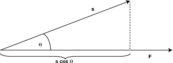
Figure 4-12. Work done is the scalar product of force and displacement
You might recognize this as the dot product between F and s, where θ is the angle between the force F and the displacement s:
![]()
Hence, if the angle θ is zero, then W = F s (because cos (0) = 1). But if θ is 90 degrees, then cos θ = 0, so W = 0. In other words, the work done by a force is zero if the displacement is perpendicular to the force.
![]() Note The resultant acceleration must always be in the direction of the resultant force. However, the resultant motion (displacement) may or may not be in the direction of the resultant force.
Note The resultant acceleration must always be in the direction of the resultant force. However, the resultant motion (displacement) may or may not be in the direction of the resultant force.
The capacity to do work: energy
Now that we know what work is, the definition of energy is simple: Energy is the capacity to do work. Take the example of the stone dropped from a height: because it can do work by falling it must possess energy just by being above the ground. This energy is called potential energy (usually abbreviated as PE, with symbol Ep). Similarly, a moving object can do work by colliding with another object, exerting a contact force during the collision and causing it to move under the action of this force. Hence, moving bodies also have energy, known as kinetic energy (usually abbreviated as KE, with symbol Ek).
In fact, work causes a transfer or conversion of energy. For example, applying a force to make an object move imparts kinetic energy to it. This causes a decrease in energy for the agent applying the force. This is expressed generally in the work-energy theorem:
Energy transferred = work done
In symbols:
![]()
Because we are equating energy and work, it follows that energy has the same unit as work: the joule (J). Like work, energy is a scalar quantity.
Energy transfer, conversion, and conservation
Just as there are many types of forces, there are also many types of energy. Examples include light energy, thermal energy, nuclear energy, and so on. But usually we will be concerned with only two forms of energy: kinetic and potential energy. At a fundamental microscopic level, all forms of energy are manifestations of these two basic forms.
Energy can be transferred from one body to another. Energy can also be converted from one form to another. Whether energy is transferred or converted, total energy is always conserved.
An example of energy transfer is the collision of two particles, where one of the particles loses KE and the other gains KE. An elastic collision is defined as one in which the total kinetic energy is conserved (KE is not converted into other forms of energy as a result of the collision); otherwise, the collision is inelastic. Therefore, if the collision is elastic, the amount of KE gained by one is exactly equal to that lost by the other.
As an example of energy conversion, a body released from a certain height loses potential energy but gains kinetic energy as it accelerates downward—its PE is converted to KE. If the body falls only under the action of the gravitational force, the gain in KE is exactly equal to the loss in PE; the total energy, kinetic plus potential, remains constant. If there are other forces, such as friction (due to air resistance), a small amount of energy is converted to thermal energy in the body and the surrounding air by doing work against friction. The total energy in all forms still remains the same. This is known as the principle of conservation of energy.
This principle is so important, let’s state it once more, in a more general way:
Principle of Conservation of Energy: Energy can be converted from one form to another or transferred from one body to another during interactions, but the total energy of a closed system is constant.
“Closed system” means a system that has no interaction outside of itself. Within the system, the interactions and exchanges can be as many or as complicated as can occur and the principle will still hold. For example, if you have hundreds of particles colliding with each other in a closed system, the principle will hold. If you have zillions of molecules interacting in an isolated gas, the principle still holds.
Because potential energy and kinetic energy are so important, let’s see how we can calculate them. Let’s start with potential energy. When we discussed the concept of work, recall that the work done by an object falling from a height h above ground was shown to be equal to mgh. Now, because work done is equal to energy transferred, the object must have possessed that amount of energy before it fell. Because it was dropped from rest at height h, its velocity was initially zero and so it had no kinetic energy to start with. Hence, its energy was all potential energy to start with. We therefore conclude that an object of mass m at a height h above the ground has an amount of potential energy given by
![]()
This is our formula for potential energy.
Let’s now work out a formula for kinetic energy. Consider the same example of the falling stone. Neglecting energy lost by friction, the kinetic energy of the stone just before it hits the ground must equal the potential energy it had initially (because it does not have any PE at the ground, so it must all have been converted to KE). So the final KE is also equal numerically to mgh. Here h is the distance that the stone has fallen. Because KE is energy possessed due to motion, we really want a formula for KE as a function of the velocity the stone has, not the displacement it has undergone. Remember the formula connecting velocity and displacement? Using v2 = u2 + 2 a . s, and noting that u = 0, a = g, and s = h, we get v2 = 2gh.
Using this, all we need to do now is replace gh by ![]() v2 and we end up with this:
v2 and we end up with this:

This is the formula for the kinetic energy of a body of mass m moving at a velocity v.
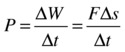
The final concept we’ll introduce is that of power. In talking about energy, we seem to have given up the concept of time. We’ve talked about work being done and energy being exchanged or transferred, but without reference to how fast it happens. Power introduces time in the energy approach.
Power is defined as the rate of doing work. In calculus notation, the power P is therefore given by the following:

Or, in discrete form:

In words, P is defined as work done divided by time taken. From this definition, the unit of power is therefore J/s. This unit has a special name. It’s called the watt (W). Another commonly used unit is the horsepower (HP). Power is a scalar quantity, just like energy.
We can reverse the last formula to obtain the work done in a time interval Δt when power P is deployed:
![]()
Power is a very useful concept for analyzing the operation of machines, such as vehicles. Suppose that a machine is doing work by exerting a force F and moving its point of application at a velocity v in the direction of F. Then, the work done is ΔW = FΔs. (Note: this is just the formula W = Fs written for small changes ΔW and Δs.)
From the definition of power as the rate of doing work, the power output of the machine is therefore this:
And because Δs/Δt = v, we end up with this formula:
![]()
So the power deployed by the machine is equal to the product of the force F it applies and the velocity v it produces.
You usually need to apply power concepts if you are simulating machines engineered by humans, such as cars and boats.
Example: A rudimentary “car” simulation
We conclude this chapter by showing you a simple example of how to apply power and energy concepts to simulate motion, without the explicit use of forces. In this example, you will apply power to a Ball object (the car) to accelerate it against frictional and other power losses, in the same manner as you press the gas pedal of your car to keep it moving.
The code for this example is in the file energy-example.js and is shown here in full:
var canvas = document.getElementById('canvas'),
var context = canvas.getContext('2d'),
var canvas_bg = document.getElementById('canvas_bg'),
var context_bg = canvas_bg.getContext('2d'),

var car;
var t;
var t0;
var dt;
var animId;
var graph;
var force;
var acc;
var g = 10;
var k = 0.5;
var animTime = 60; // duration of animation

var powerLossFactor=0.1;
var powerApplied=50;
var ke;
var vmag;
var mass;
var applyThrust=false;

window.onload = init;

function init() {
     car = new Ball(15,'#000000',1,0,true);
     car.pos2D = new Vector2D(50,50);
     car.velo2D=new Vector2D(20,0);
     car.draw(context);
     mass = car.mass;
     vmag = car.velo2D.length();
     ke = 0.5*mass*vmag*vmag;
     window.addEventListener('keydown',startThrust,false);
     window.addEventListener('keyup',stopThrust,false);
     setupGraphs();

     t0 = new Date().getTime();
     t = 0;
     animFrame();
};

function setupGraphs(){
     //graph = new Graph(context,xmin,xmax,ymin,ymax,xorig,yorig,xwidth,ywidth);
     graph= new Graph(context_bg,0,60,0,50,100,550,600,400);
     graph.drawgrid(5,1,5,1);
     graph.drawaxes('time (s)','velocity (px/s)'),
}

function startThrust(evt){
     if (evt.keyCode==38){
          applyThrust = true;
     }
}
function stopThrust(){
     applyThrust = false;
}

function animFrame(){
     animId = requestAnimationFrame(animFrame,canvas);
     onTimer();
}
function onTimer(){
     var t1 = new Date().getTime();
     dt = 0.001*(t1-t0);
     t0 = t1;
     if (dt>0.2) {dt=0;}; // fix for bug if user switches tabs
     t += dt;
     //console.log(dt,t,t0,animTime);
     if (t < animTime){
          move();
     }else{
          stop();
     }
}
function move(){
     moveObject();
     applyPower();
     updateVelo();
     plotGraphs();
}

function moveObject(){
     car.pos2D = car.pos2D.addScaled(car.velo2D,dt);
     context.clearRect(0, 0, canvas.width, canvas.height);
     car.draw(context);
}
function applyPower(){
     if (applyThrust){
          ke += powerApplied*dt;
     }
     ke -= powerLossFactor*vmag*vmag*dt;
}
function updateVelo(){
     vmag = Math.sqrt(2*ke/mass);
     car.vx = vmag;
}
function plotGraphs(){
     graph.plot([t], [car.vx], '#ff0000', false, true);
}
function stop(){
     cancelAnimationFrame(animId);
}
Most of the code should be familiar from previous examples. The init() method includes extra code that sets up keydown and keyup event listeners. The corresponding event handlers set the value of a Boolean variable applyThrust to true if the up-arrow key is pressed and to false otherwise.
Some convenience variables are used in the code: mass (the mass of the particle), vmag (its velocity magnitude), ke (its kinetic energy), powerApplied (the applied power), and powerLossFactor (a coefficient we use to calculate the power loss due to friction and other factors). The values of vmag and ke are initialized in init(). We have given the ball an initial velocity of 20 px/s in the x-direction. The mass of the ball is 1 unit.
The most important, and novel, parts of the code are the two methods applyPower() and updateVelo(), which are called at every timestep within the move() method.
In applyPower(), we are updating the kinetic energy of the ball. The applyThrust Boolean variable tells us if the up-arrow key is pressed; if so, the KE is updated by multiplying the power by the time interval dt. What we are doing here is applying this formula:
![]()
You might not immediately recognize this formula, but it is obtained by equating the work done ΔW = PΔt with the kinetic energy gained according to the work-energy theorem, as discussed earlier. Conceptually, what is happening is that the applied power is doing mechanical work on the ball, which results in an increase in its kinetic energy.
In applyPower(), you will notice that we also reduce the kinetic energy of the ball by an amount equal to powerLossFactor*vmag*vmag*dt. This is equivalent to applying a power loss given by the following, where k is a constant corresponding to powerLossFactor:
![]()
This formula comes from applying the formula P = F v we saw in the last section and modeling the total of all resistive forces (such as friction and drag) by F = –k v, as a force proportional to the velocity of the ball (see Chapter 7). This is a crude approximation, but it will do for the purpose of our simple example.
The updateVelo() method first computes the velocity magnitude from the updated kinetic energy by this formula, which is obtained by reversing the formula for kinetic energy Ek = ![]() m v2:
m v2:
![]()
It then updates the ball’s velocity accordingly.
There is also code for setting up a Graph instance and plotting a graph of the horizontal velocity component of the ball as the simulation progresses. These pieces of code are straightforward, so we will not go into them here.
If you run the code, you will find that the ball starts moving, but its velocity is gradually reduced, owing to the effect of the power loss. If you then press and hold down the up-arrow key, the applied power will cause an increase in the ball’s KE, making it accelerate. If the power is applied continuously, eventually the velocity will tend to a constant value, but if the up-arrow key is released, the velocity will reduce again, as shown in Figure 4-13. This behavior mirrors the operation of a car accelerator in a simple way.
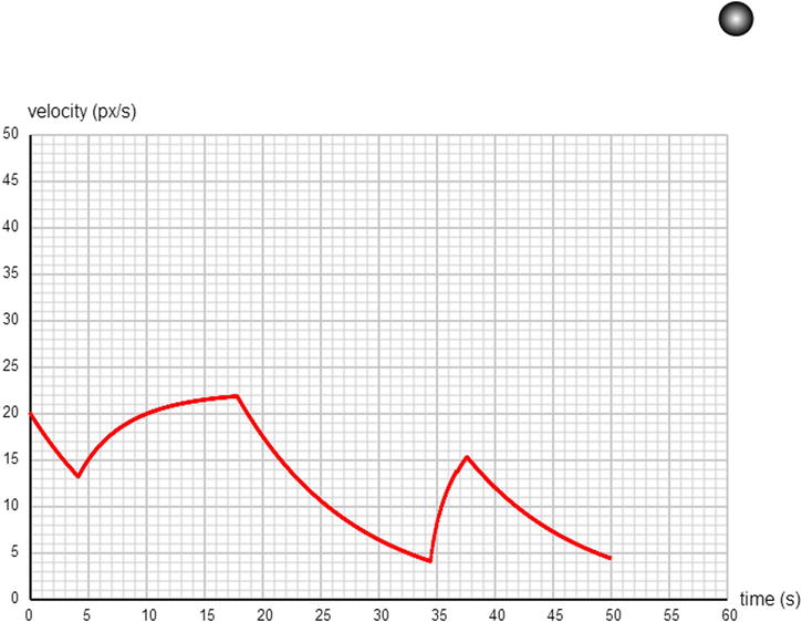
Figure 4-13. A rudimentary car simulation
Summary
That was another long overview chapter, and you’ve now learned an awful lot of physics concepts. This chapter completes Part I of the book. The next chapter will bring together what you’ve learned so far to lay out the principles of how to simulate a wide range of forces and motions.
Get ready for the real action!