![]()
Numerical Integration Schemes, Accuracy, and Scaling
In the previous two parts of this book we have covered a lot of physics. In the process we have largely managed to avoid getting into complex numerical issues. In this chapter we will focus on the important subject of numerical integration schemes and considerations of numerical stability and accuracy. Because no new physics will be presented, there won’t be any new simulations in this chapter, but just some simple code examples to test the different schemes. At the end of the chapter we also include a short section on building scale models.
Numerical integration is a branch of numerical analysis that deals with the solution of differential equations. An integration scheme is a particular method for doing numerical integration in a form that you can readily write into code. We need an integration scheme to simulate motion because it involves solving Newton’s second law of motion (which is a differential equation; see Chapter 5).
Topics covered in this chapter include the following:
- General principles: We begin by stating the general problem to be solved and explain the different types of integration schemes available and their characteristics.
- Euler integration: This is the simplest integration method and is the one we have been using throughout the book so far. It is fast and very easy to code, but it is inaccurate and can be unstable, which can lead to problems with some types of simulations.
- Runge-Kutta integration: This method is much more accurate than the Euler scheme, but it involves a lot of calculations and can therefore slow down your simulation. It is particularly suited to highly accurate simulations.
- Verlet integration: This method is not as accurate as Runge-Kutta, but is generally better than the Euler scheme. It is well suited to a number of game programming and animation applications.
- Tips for achieving accuracy: This section reviews some of the factors you need to take into account if you want to create a simulation that needs to be highly accurate.
- Building scale models: Numerical accuracy is not the only consideration when you are building realistic simulations. This section discusses how to choose units and parameter values to create a scale model of the system you are trying to simulate.
General principles
Before we look at specific integration schemes, it is useful to start by posing the problem of numerical simulation in a general way and then looking at how numerical integration approaches its solution. We then discuss the general characteristics of integration schemes and review some terminology associated with different types of schemes.
Statement of the problem
Numerical integration is a method to solve a problem. So what is the problem we are trying to solve?
Motion of a particle as an initial-value problem
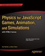
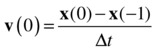
To simplify the discussion, consider the problem of simulating the motion of a single particle under the action of forces. Suppose the particle starts out at a location given by its initial position vector x(0) with respect to an origin O and with an initial velocity v(0) (see Figure 14-1). The problem is then to determine the trajectory as a function of time. Mathematically, this is equivalent to determining the position and velocity vectors x(t) and v(t) as a function of time. This is called an initial-value problem.
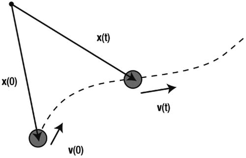
Figure 14-1. The initial-value problem for particle motion simulation
In this problem, the velocity of the particle v could itself be changing in time (in other words, the particle could be accelerating). That is why we need Newton’s second law:

Knowing the acceleration at any time then allows us to calculate the velocity v by integrating the equation that defines acceleration:

Similarly, applying the definition of velocity, we can obtain the position by integrating the velocity in time:

As discussed in Chapter 5, these differential equations can sometimes be solved analytically to give closed-form expressions for x(t) and v(t) as functions of time. In computer simulation, the integration needs to be done numerically.
Numerical integration means that the position and velocity of the particle, which change continuously, can be calculated and updated only in small discrete steps. To do this, we must first discretize the equations of motion just shown.
Numerical discretization and difference schemes
You saw an example of the discretization procedure back in Chapter 3 when we discussed the numerical calculation of gradient functions in general mathematical terms. You may want to refer to the section “Simple calculus ideas” there for a refresher.
In the current context, you can apply numerical discretization to the previous two equations to convert them into a form that can be put into code and solved on a computer.
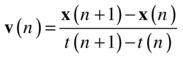
This is done by approximating the derivatives in those equations by algebraic fractions. For example, we can approximate the acceleration dv/dt using small changes Δv and Δt in v and t like this:
The next step is to represent the discrete step changes Δv and Δt in terms of values at definite times because that is what you know (or rather what your computer knows). This can be done in different ways, known as difference schemes.
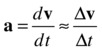
As an example, you can take Δt to be the time at the next timestep minus the current time, and similarly for the velocity interval Δv. This gives a forward difference scheme, as discussed in Chapter 3 (note that n here denotes the timestep number):
Similarly, the velocity can be approximated by a forward difference scheme in the following way:
Now you’ve converted the differential equations into algebraic equations that you can understand and manipulate easily. More importantly, it’s in a form that a computer can calculate. This is the role of discretization.
But before you can put anything into code, there is one more step: you need to convert the preceding difference scheme to an integration scheme.
Numerical integration and integration schemes
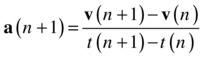
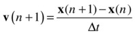
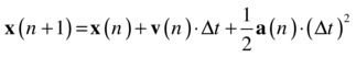
Numerical integration was also introduced in general terms in Chapter 3. The key idea is that we need to find the velocity and position at the new time in terms of those values at the old time. So, just as we did in Chapter 3, we manipulate the previous equations to give the following expressions for v(n+1) and x(n+1), in which we have written the time difference t(n+1) – t(n) as Δt (the timestep):
![]()
![]()
This gives a forward integration scheme known as the Euler scheme, as you know. With these equations, you can obtain the new velocity and position of your particle in terms of its velocity and position at the previous timestep. You can now put these equations directly into code and simulate the motion of the particle by repeating that calculation at each timestep. This will give you a discrete approximation of the true trajectory of the particle, as shown schematically in Figure 14-2. A good simulation means that this approximated trajectory is as close to the real one as needed for your particular purpose. How good the approximation turns out to be will depend on a number of factors, including the following:
- Physics of the problem: Effectively, this is captured by how the acceleration a varies with time. Some physical problems are easier to simulate accurately than others, especially if the acceleration does not vary much with time.
- Simulation timestep: Generally, the smaller the timestep the better the approximation will be. But reducing the timestep comes at a cost because your simulation may run more slowly. Referring to Figure 14-2, smaller timesteps mean that the distance between the dots is reduced and that the approximated curve is closer to the true one.
Integration scheme: The choice of integration scheme generally has a significant effect on the accuracy, stability, and speed of execution of your simulation. But there is often a trade-off between these desirable characteristics.

Figure 14-2. Numerical integration gives an approximation of the true trajectory
Characteristics of numerical schemes
When you are deciding which integration scheme to use, there is a set of characteristics that you need to bear in mind, as they determine how “good” that scheme is and how well suited it is to the application you have in mind. We’ll briefly discuss some of these characteristics separately, but remember that they are connected.
Consistency of a numerical scheme is the property that the numerical scheme is consistent with the original differential equation in the sense that it approximates the differential equation. Formally, in the limit of indefinitely small timesteps, the numerical solution should be identical to the true solution of the differential equation. This can be viewed as a necessary condition for any numerical scheme. If it’s not true, the scheme will give the wrong physics and be essentially useless.
In the previous chapter you saw a spectacular example of numerical instability as the rope simulation “blew up” when the spring stiffness was too high. Formally, the stability of a numerical scheme is its capability to reduce errors (or “perturbations,” as they are usually called) over time. A scheme is stable if an error or perturbation at any time decays with time; it is unstable if the error grows with time. A scheme can be conditionally stable (meaning that it is stable under certain conditions) or unconditionally stable (always stable, regardless of the conditions).
Convergence is the requirement that as we reduce the timestep, the resulting numerical solution should approach the true solution. Consistency is a necessary condition for convergence, but not a sufficient condition. Again, clearly a numerical scheme is of no use if it is not convergent. For convergence, a scheme must also be stable.
Replacing a differential equation by finite differences inevitably introduces errors (known as discretization errors). Needless to say, it is desirable to keep these errors as small as possible. The accuracy of a numerical scheme determines how small or large these errors will be. The timestep also has an important effect on the numerical errors; errors are generally smaller the smaller the timestep (if the scheme is convergent). The order of a numerical scheme determines how quickly the errors diminish as you reduce the timestep. A first-order scheme has an error that is proportional to the timestep Δt, a second-order scheme has an error proportional to (Δt)2, and so on. Therefore, as the timestep Δt is reduced, a second-order scheme will converge faster to the real solution, making it more accurate.
The efficiency of a numerical scheme quantifies how quickly (in wall clock time) it can compute a solution per unit simulation time. For the same timestep, the more complex a numerical scheme is, the lower is its efficiency because it has to perform a greater number of calculations and associated operations to produce a given solution per timestep. More accurate schemes are usually more complex and therefore less efficient. There is, therefore, usually a trade-off to achieve between accuracy and efficiency. However, in an actual implementation, the overall efficiency of a numerical method depends on the size of timestep that it can allow while preserving stability and accuracy. It could turn out that a simple scheme requires a much larger timestep to remain stable than a more complicated one, making it effectively less efficient in terms of overall computing time per simulation time.
Types of integration schemes
The terminology of numerical analysis can sound confusing because of the plethora of schemes, their associated names, and the different ways to classify them. Following are very brief descriptions of some of the terminology associated with the classification of integration schemes. Note that the categories mentioned here are not mutually exclusive; they overlap.
- Forward/backward schemes: You may come across scheme names such as forward Euler and backward Euler. These names show that the scheme is derived from a corresponding forward or backward difference scheme.
- Implicit/explicit schemes: An explicit scheme is one in which the values of the state variables at the new timestep are computed in terms of only the variables at the previous timestep; this makes an explicit scheme straightforward to apply. In an implicit scheme, an equation involving variables at both the old and the new timestep must be solved to calculate the variables at the new timestep; this makes such schemes less efficient.
- Single-step/multistep methods: A single-step method uses information from a single previous timestep to calculate variables at the new timestep. A multistep method uses information from more than one previous timestep.
- Predictor-corrector methods: As its name suggests, a predictor-corrector method involves two stages: a step that predicts a value at the new timestep, followed by another step that applies a correction to the estimated value.
- Runge-Kutta methods: This refers to a class of higher-order methods that proceed by employing intermediate stages and can be explicit as well as implicit. We will consider two examples of such methods, including the fourth-order Runge-Kutta (RK4) method, which is often referred to simply as the Runge-Kutta method.
A simple example to demonstrate different integration schemes
In the next sections we discuss a number of different schemes and then write code that will implement them. It would be helpful to be able to switch between different schemes easily, which would be convenient for comparing different schemes and for choosing an appropriate scheme for each problem.
Enabling that switching is best demonstrated in a simple example that modifies the structure of the animation code we have been using in most of the examples in this book so far. Specifically, we will modify the basic forces-test.js example from way back in Chapter 5, which demonstrated the motion of a ball under the forces of gravity and drag, to handle switching. We call the modified file schemes-test.js. The beginning of the code looks like this:
var canvas = document.getElementById('canvas'),
var context = canvas.getContext('2d'),

var ball;
var m = 1;
var g = 10;
var k = 0.1;
var t, t0, dt;
var force, acc;
var animId;
var animTime = 10;

window.onload = init;

function init() {
     ball = new Ball(15,'#0000ff',m,0,true);
     ball.pos2D = new Vector2D(50,400);
     ball.velo2D = new Vector2D(60,-60);
     ball.draw(context);
     t0 = new Date().getTime();
     t = 0;
     animFrame();
};

function animFrame(){
     animId = requestAnimationFrame(animFrame,canvas);
     onTimer();
}
function onTimer(){
     var t1 = new Date().getTime();
     dt = 0.001*(t1-t0);
     t0 = t1;
     if (dt>0.2) {dt=0;};
     t += dt;
     if (t < animTime){
          move();
     }else{
          stop();
     }
}
function stop(){
     cancelAnimationFrame(animId);
}
function move(){
     myFavoriteScheme(ball);
     context.clearRect(0, 0, canvas.width, canvas.height);
     ball.draw(context);
}
function calcForce(pos,vel){
     var gravity = Forces.constantGravity(m,g);
     var drag = Forces.linearDrag(k,vel);
     force = Forces.add([gravity, drag]);
}
function getAcc(pos,vel){
     calcForce(pos,vel);
     return force.multiply(1/m);
}
function myFavoriteScheme(obj){
     //scheme-specific code goes in here
}
The key structural changes to the code are indicated with boldface type. The calcForce() method now takes two arguments, pos and vel, which reference position and velocity vectors. This will be needed because some schemes require the evaluation of the acceleration (and hence the force) at different times. In the listed example the pos parameter is not used, but it may be needed in future examples and so is included for generality. Those schemes will do that evaluation by calling the private getAcc() method, which calculates the acceleration, also with position and velocity vectors as arguments. The move() method will call the method that implements the integration scheme. All the scheme-specific code will be in its own method, here named generically as myFavoriteScheme(). In this way it will be easy to implement new schemes and to switch between schemes. Note that we are only applying the changes to the linear motion because we will only use the new integration schemes for particle motion; as a further exercise you could also implement them on the rotational motion along the same lines.
We have talked about and used the Euler integration scheme a lot in this book, so you are very familiar with it by now. But what you might not know is that there are several different versions of the Euler scheme. Let’s take a look at some of them and their properties.
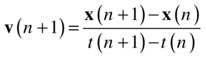
The Euler integration scheme that we derived earlier in this section from the forward difference scheme is called (appropriately enough) the forward Euler scheme. And because it is an explicit scheme, it is also known as the explicit Euler scheme. Here are the equations again:
![]()
![]()
Because it is simple, the explicit Euler scheme is fast, but it has only first-order accuracy and is often unstable.
Note that when implementing this scheme in code, we update the position based on the current velocity before updating the velocity based on the current acceleration, to be consistent with the previous equations.
The relevant code in the file schemes-test.js is in the EulerExplicit() method, which looks like this:
function EulerExplicit(obj){
     acc = getAcc(obj.pos2D,obj.velo2D);
     obj.pos2D = obj.pos2D.addScaled(obj.velo2D,dt);
     obj.velo2D = obj.velo2D.addScaled(acc,dt);
}
The explicit Euler scheme was obtained by starting from a forward difference approximation to the derivative. You can instead start from a backward difference scheme:
Rearranging these difference equations then gives the following:
![]()
![]()
This looks similar to the corresponding equation for the explicit Euler scheme, except for one crucial difference: the right sides of those equations contain the acceleration as well as the velocity at the new timestep. We therefore have an implicit equation that needs to be solved first before we can obtain the velocity at the new timestep. This involves further calculations, which make implicit schemes less efficient (as well as a pain to code up!). A major advantage of the implicit scheme is that it is unconditionally stable. If you want to make sure that your simulation will never blow up, it’s worth considering using an implicit scheme. But because we don’t use the implicit Euler scheme in this book, we won’t bother coding it up.
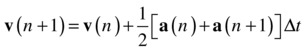
The semi-implicit Euler scheme, as its name suggests, is somewhere between the explicit and implicit Euler schemes. In one common variant, the velocity is advanced based on the acceleration at the previous timestep, as in the explicit scheme, but the position is advanced based on the updated velocity at the new timestep, as in the implicit scheme:
![]()
![]()
The advantage of the semi-implicit scheme is that it is more stable than the explicit scheme and also conserves energy. This energy-conserving property makes it more accurate than the explicit scheme, although it is still first-order.
Compared with the implementation of the explicit scheme, the semi-implicit scheme is simple to implement. You just reverse the order in which you update the position and velocity. Here is the corresponding function EulerSemiImplicit():
function EulerSemiImplicit(obj){
     acc = getAcc(obj.pos2D,obj.velo2D);
     obj.velo2D = obj.velo2D.addScaled(acc,dt);
     obj.pos2D = obj.pos2D.addScaled(obj.velo2D,dt);
}
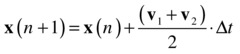
There is another variant of the semi-implicit Euler scheme (with properties similar to the first version), in which the position is advanced based on the current velocity instead of the updated velocity, and the velocity is advanced based on the updated acceleration (and therefore at the updated position):
![]()
![]()
Note that because the acceleration potentially depends on the position and must be evaluated at the new time, the position must be updated first in code. This version of the semi-implicit Euler scheme is the one that we have been using throughout most of the book, and it has mostly worked quite well, at least for the purpose of creating simple demos of various types of physics effects.
We’ve coded this in the function EulerSemiImplicit2():
function EulerSemiImplicit2(obj){
     obj.pos2D = obj.pos2D.addScaled(obj.velo2D,dt);
     acc = getAcc(obj.pos2D,obj.velo2D);
     obj.velo2D = obj.velo2D.addScaled(acc,dt);
}
Comparing the explicit and semi-implicit Euler schemes
To compare the explicit and semi-implicit Euler schemes, let’s put together a very simple simulation of a particle oscillating under the effect of a spring force. The file spring.js sets up a particle and a center toward which a spring force acts, and it creates two other particles at the points where its trajectory should theoretically end. The calcForce() method then applies the spring force and simulates the motion of the moving particle, tracing out its trajectory. There is nothing new in terms of physics or coding in those files, so we won’t list any code here. But the key point is that you can change the integration scheme in the move() method.
Run the simulation in turn with the EulerExplicit(), EulerSemiImplicit(), and EulerSemiImplicit2() methods. You can choose an integration scheme by uncommenting the relevant line in the moveObject() method in springs.js and commenting out the other lines (as an alternative, you may want to modify the code to run multiple schemes at the same time). You will find that the particle oscillates as expected and remains nicely within the bounds of the endpoints with either of the two semi-implicit schemes. The semi-implicit Euler method nearly conserves energy; it’s a so-called symplectic method. However, the explicit Euler scheme behaves very badly: the oscillations grow larger and larger (see Figure 14-3). The simulation blows up: explicit Euler creates energy! The stability is improved if you introduce some physics that can remove energy, such as drag or friction. However, the scheme can’t simulate pure periodic oscillatory motion.

Figure 14-3. The explicit Euler scheme is too unstable to simulate spring motion properly
As another test of the stability of these schemes, try running the rope simulation from the previous chapter with the explicit Euler scheme by changing the order of the position and velocity updates in the move() method. This is done in the file rope-explicit-euler.js: it’s not a pretty sight! The explicit Euler scheme can’t simulate the rope even at a much lower stiffness. Interestingly, even the first version of the semi-implicit scheme does not do as well as the second version; it becomes unstable for much smaller values of the stiffness. By comparison, the second version of the semi-implicit scheme is quite robust, although it also eventually fails, as you saw in Chapter 13.
Why use Euler and why not?
Many programmers use nothing but Euler integration, whereas others keep as far away from Euler as they can. So should you use Euler or not?
To answer this question wisely, it is important to distinguish between the different versions of the Euler method. People often talk of the Euler scheme as if there were only one. But we’ve just seen that different versions of Euler have very different properties, which can lead to vastly different performance depending on the nature of your simulation. There is bad Euler and there is better Euler. You should definitely avoid the bad, explicit Euler. Semi-implicit Euler is actually not that bad (after all, we’ve survived for most of the book with it!). It is as easy to code as the explicit Euler scheme, but has much nicer properties. In code, the difference between the explicit and semi-implicit Euler schemes simply amounts to swapping the order in which you compute variables (so be careful!). So there really is no reason to use the explicit Euler scheme. The semi-implicit Euler scheme is widely used in rigid-body physics engines.
If you need absolute stability, the fully implicit Euler scheme is worth considering, although we haven’t really shown you how to solve an implicit equation. But now that you have a better insight into numerical schemes, it shouldn’t be hard to figure it out from books or online sources. The extra computational cost involved in solving the resulting implicit equation makes the implicit Euler scheme seem less attractive in terms of efficiency. But you can use large timesteps without worrying about numerical instability, which would improve the efficiency. However, large timesteps would then result in poor accuracy, especially given that Euler is only first-order. That’s probably fine if accuracy is not important compared to stability (for example, if you just want your simulation not to blow up, without worrying about its accuracy).
However, if you really need accuracy, the first-order Euler schemes we have discussed won’t serve you well. What you probably need then is something like a Runge-Kutta scheme.
Runge-Kutta schemes are more complex than the Euler scheme, but they pay off in terms of considerably greater accuracy. If accuracy is critical for your simulation, you should seriously consider Runge-Kutta. This accuracy does come at a performance price, though, especially if you opt for the higher-order schemes. We’ll describe two of the most popular Runge-Kutta schemes.
Second-order Runge-Kutta scheme (RK2)
The second-order Runge-Kutta method (RK2) is also known as Heun’s method or the improved Euler method. It is a two-stage predictor-corrector method that uses the explicit Euler’s method as predictor and a so-called trapezoidal method as corrector. Here are the equations defining the method:
![]()
![]()
![]()
![]()
![]()
![]()

The temporary variables p1, v1, and a1 are the initial position, velocity, and acceleration vectors; similarly, p2, v2, and a2 are the corresponding variables at the end of the timestep as computed by the forward Euler scheme. That’s the predictor part. The last two equations apply the corrector by updating the position and velocity using (respectively) the average velocity and average acceleration over the timestep interval.
RK2 is more accurate than Euler because the Euler scheme uses only the velocity and acceleration at the old timestep to work out the new velocity and position of the particle. That would be fine if there were no acceleration, so that the velocity remained constant during a timestep, but both the velocity and the acceleration could be changing. For example, for a projectile the velocity changes both in magnitude and in direction. The Euler scheme takes into account the velocity only at the beginning of a timestep, but the RK2 scheme takes the average of the velocities at the beginning and the end of the timestep. So the position at the end of the timestep as predicted by RK2 ends up being closer to the real position.
The accuracy of this method is second order, so it is significantly more accurate than the Euler method. Here is the relevant RK2() function:
function RK2(obj){
     var pos1 = obj.pos2D;
     var vel1 = obj.velo2D;
     var acc1 = getAcc(pos1,vel1);
     var pos2 = pos1.addScaled(vel1,dt);
     var vel2 = vel1.addScaled(acc1,dt);
     var acc2 = getAcc(pos2,vel2);
     obj.pos2D = pos1.addScaled(vel1.add(vel2),dt/2);
     obj.velo2D = vel1.addScaled(acc1.add(acc2),dt/2);
}
The RK2() function involves a few more lines of code than the semi-implicit Euler schemes. For the same timestep an increase in accuracy is therefore achieved at the expense of reduced speed.
Fourth-order Runge-Kutta scheme (RK4)
The fourth-order Runge-Kutta scheme (RK4) is the best-known Runge-Kutta scheme, and is often called the Runge-Kutta scheme. As its name suggests, it is fourth-order accurate. So if you halve the timestep, the error should be reduced by a factor of one-sixteenth! The idea is similar to that of RK2, but there are more intermediate steps, and the intermediate variables and their averages are computed differently. Here is the full set of equations:
![]()
![]()
![]()
![]()
![]()
![]()
![]()
![]()
![]()
![]()
![]()
![]()

Following is the corresponding RK4() method:
function RK4(obj){
     var pos1 = obj.pos2D;
     var vel1 = obj.velo2D;
     var acc1 = getAcc(pos1,vel1);
     var pos2 = pos1.addScaled(vel1,dt/2);
     var vel2 = vel1.addScaled(acc1,dt/2);
     var acc2 = getAcc(pos2,vel2);
     var pos3 = pos1.addScaled(vel2,dt/2);
     var vel3 = vel1.addScaled(acc2,dt/2);
     var acc3 = getAcc(pos3,vel3);
     var pos4 = pos1.addScaled(vel3,dt);
     var vel4 = vel1.addScaled(acc3,dt);
     var acc4 = getAcc(pos4,vel4);
     var velsum = vel1.addScaled(vel2,2).addScaled(vel3,2).add(vel4);
     var accsum = acc1.addScaled(acc2,2).addScaled(acc3,2).add(acc4);
     obj.pos2D = pos1.addScaled(velsum,dt/6);
     obj.velo2D = vel1.addScaled(accsum,dt/6);
}
That’s a lot of calculations to do in a single timestep! So let’s see what RK4 can do for us. We’ll compare the Euler, RK2, and RK4 methods for three different problems.
Stability and accuracy of RK2 and RK4 compared with Euler
To check the stability of RK2 and RK4, you can repeat the springs test, using the RK2() and RK4() methods. You’ll find that the oscillatory motion is perfectly simulated by both: there isn’t even a slight decrease or increase in the amplitude of oscillation (and therefore of energy) as far as the eye can tell (if you want, you can perform more quantitative tests by plotting a graph).
To test the accuracy of the schemes and compare it with that of the previous schemes in a simple way, let’s put together a simple orbit simulation. The file is called orbits.js. Again there is nothing that you haven’t seen in earlier files, and we won’t list any code from it here. The test is that the orbits should close on themselves; if they don’t, the scheme is introducing significant errors.
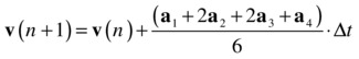
Run the code with different integration schemes as before. With the explicit Euler integrator, the orbit will end up all over the place: it never closes on itself (see Figure 14-4). That should be enough to convince you never to use the explicit Euler scheme!
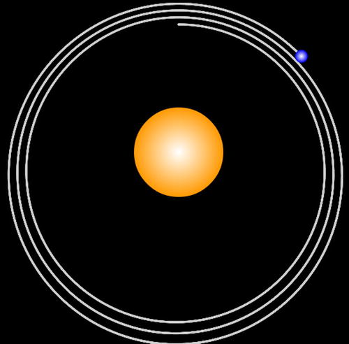
Figure 14-4. The explicit Euler scheme is too inaccurate to produce a closed orbit
All the other schemes do a pretty decent job. But if you were to run the simulation for a long time, you would find that even the semi-implicit Euler schemes start losing accuracy and tracing slightly non-overlapping circles because they are only first-order accurate (see Figure 14-5). By comparison, we ran the RK4 scheme for a much longer duration, but could not notice any loss of accuracy. The RK2 scheme is intermediate in accuracy between the semi-implicit Euler scheme and the RK4 scheme. For this simple example you will hardly notice any difference between RK2 and RK4.
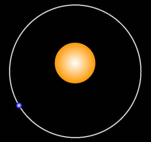
Figure 14-5. The semi-implicit Euler scheme accumulates errors after a few orbits
The third and final class of integration schemes that we’ll discuss is called Verlet integration. Originally developed for handling complex and variable molecular dynamics simulations because of its stability properties, the approach is now widely used in game programming and animation.
Verlet integration is employed in so-called Verlet systems to simulate the motion of particles subject to constraints. This technique can be applied to connected structures as in ragdoll physics, forward and inverse kinematics, and even rigid body systems. We do not have space to explore this approach. We mention Verlet systems merely to distinguish them from the Verlet integration scheme because they are sometimes confused: Verlet systems are named as such because they use the Verlet integration scheme. But the scheme itself is completely independent of that modeling approach; in fact, it can be used with any other approach, such as the rigid body dynamics discussed in Chapter 13.
Verlet integration schemes are generally not as accurate as RK4 but, on the other hand, are very efficient in comparison. Let’s take a look at two common variants of the method: Position Verlet and Velocity Verlet.
In the Position Verlet method, also known as the Standard Verlet method, the velocity of a particle is not stored. Instead, the last position of the particle is stored, and its velocity can then be computed as needed by subtracting the last position from the current position and dividing by the timestep.
Just as the explicit Euler scheme can be derived starting from the forward difference approximation of the first derivative, the standard Verlet scheme can be derived from the central difference approximation to the second derivative (see Chapter 3). We won’t show the derivation here but only quote the final result:
![]()
This equation gives the position at the new timestep in terms of the positions at the previous two timesteps without using the velocity.
If desired, the velocity can be computed from the positions—for example, using backward differencing:
Alternatively you can use the central differencing scheme, because the previous position is also known, to give a more accurate estimate of the velocity:

One problem with the Position Verlet equation as given previously is that it assumes that the timestep is constant. But in general the timesteps in your simulation could be variable. In fact, the timesteps will usually vary slightly in your JavaScript simulations. To allow for variable timesteps, a modified version of the equation is used:
![]()
In this equation, Δt(n) denotes the current timestep, and Δt(n-1) denotes the previous timestep. This form can be called the time-corrected or time-adjusted Position Verlet scheme.
Another potential problem that arises in the implementation of the Position Verlet scheme is the specification of the initial conditions. Because the scheme does not use velocity but the position at the previous timestep, you cannot directly specify the initial velocity together with the initial position as you would normally do. Instead, you need to specify the initial position x(0) as well as the previous position x(–1) before the initial position! That might sound like nonsense, but you can actually infer the value of that hypothetical position from the initial velocity by applying the backward difference formula for the velocity given previously. Setting n = –1 in that formula gives the following:
Solving this equation for x(–1) then gives this:
![]()
We can now write a PositionVerlet() function as follows:
function PositionVerlet(obj){
     var temp = obj.pos2D;
     if (n==0){
          acc = getAcc(obj.pos2D,obj.velo2D);
          oldpos = obj.pos2D.addScaled(obj.velo2D,-dt).addScaled(acc,dt*dt/2);
          olddt = dt;
     }
     acc = getAcc(obj.pos2D,obj.velo2D);
     obj.pos2D = obj.pos2D.addScaled(obj.pos2D.subtract(oldpos),dt/olddt).addScaled(acc,dt*dt);
     obj.velo2D = (obj.pos2D.subtract(oldpos)).multiply(0.5/dt);
     oldpos = temp;
     olddt = dt;
     n++;
}
Note that we have new variables oldpos and olddt for storing the previous position and the previous timestep. There is also a variable n that represents the number of timesteps that have elapsed since the last call to that function. As you can see from the code, the first time the function is called, the position x(–1) is set.
One of the problems with the Position Verlet method is that the velocity estimation is not very accurate. The Velocity Verlet method fixes this, albeit at some cost in efficiency. The Velocity Verlet is the more commonly used version of the two. The scheme equations are these:
Comparing the first equation with the corresponding equation in the Euler scheme shows that we now have an additional term that includes the acceleration. The Euler scheme therefore assumes that the acceleration is zero in the interval of one timestep, whereas the Velocity Verlet method takes into account the acceleration but assumes it is constant during that interval. Perhaps you recall the equation s = ut + ½ at2 from Chapter 4. The equation for the position update in the Velocity Verlet is exactly of that form (the displacement is s = x(n+1) – x(n)).
Also note that the velocity update equation uses the average of the acceleration at the old and the new timestep rather than the acceleration just at the old timestep. Hence, it is a better approximation of the velocity. For these reasons the Velocity Verlet scheme is more accurate than the Euler scheme, as well as having other nice properties such as greater stability and conservation of energy.
Here is the VelocityVerlet() method:
function VelocityVerlet(obj){
     acc = getAcc(obj.pos2D,obj.velo2D);
     var accPrev = acc;
     obj.pos2D = obj.pos2D.addScaled(obj.velo2D,dt).addScaled(acc,dt*dt/2);
     acc = getAcc(obj.pos2D,obj.velo2D);
     obj.velo2D = obj.velo2D.addScaled(acc.add(accPrev),dt/2);
}
Testing the stability and accuracy of the Verlet schemes
You can now run the spring and orbit simulations using the Verlet schemes. You should find that they do quite a good job in both cases. Verlet schemes are stable, but they are less accurate than RK4.
A simple test to illustrate the differences in the accuracy of all the different schemes can be done by performing a simulation for a problem with a known analytical solution, against which the numerical solutions can then be compared. You might recall that we did such a test for the Euler scheme for a projectile simulation back in Chapter 4. Let’s do something similar now for all the different schemes.
The file projectile.js contains the code. Once again we won’t show any code listings because you’ve seen similar code tons of times by now. The main point is that it creates a ball and initializes its position and velocity such that the ball is thrown upward at an angle, and then subjects the ball to gravity.
Run the simulation with different integrators. The code plots the analytical trajectory as well as the numerically computed trajectory (which, of course, the ball follows). You will find that the time-corrected Position Verlet and all the Euler integrators give a trajectory that deviates slightly from the analytical trajectory (see Figure 14-6). On the other hand, the trajectories predicted using the Velocity Verlet, RK2, and RK4 schemes are so close to the analytical trajectory that they cannot be distinguished. Like RK2, the Velocity Verlet scheme is a second-order scheme. Note that these comparisons are for a specific problem, involving constant acceleration. Different schemes might be more or less accurate with different problems.
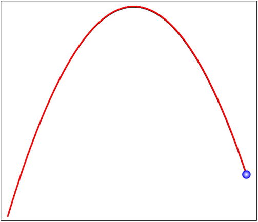
Figure 14-6. Projectile trajectory simulated with Position Verlet scheme (slightly lower curve)
Finally, you might want to check how well the standard Position Verlet scheme does without the time correction. To do this, replace the line of code that updates the position in PositionVerlet() with the following one:
obj.pos2D = obj.pos2D.add(obj.pos2D).subtract(oldpos).addScaled(acc,dt*dt);
If you then run the code you will find that the simulation gets it completely wrong! The message is that time correction is essential if you have variable timesteps in your simulation.
Tips for achieving accuracy
If you want to build very accurate simulations, you need to consider several aspects carefully. We briefly review here what you have learned about the subject in this chapter as well as in previous chapters.
Choosing an appropriate integration scheme
We have spent a lot of time in this chapter discussing numerical integration schemes and their characteristics such as accuracy and stability. Therefore, there is not much more to be said here. Just to reiterate briefly, the usual Euler scheme is not very accurate, being only a first-order scheme; the fourth-order Runge-Kutta scheme, RK4, is generally a good choice for simulations where accuracy is important, although this comes at the price of reduced efficiency. The RK2 and Velocity Verlet schemes offer a good compromise between accuracy and speed, being second-order (and therefore more accurate than the Euler scheme) and at the same time being substantially simpler than RK4.
Together with the integration scheme, you need to choose an appropriate timestep for your simulation. Numerical schemes are more accurate with smaller timesteps. Higher-order schemes such as RK4 converge faster than lower-order schemes such as Euler. This implies that RK4 is more accurate for a given timestep. You can control the timestep to some extent. However, there is a limit to how small the timestep can be because the actual time interval between timer events includes the time it takes to execute all the code within the event handler. Therefore, if your simulation is complex and involves lots of calculations or animation, the actual timestep may be substantially larger than what you specify in the timer.
Some simulations are so complex that the calculations cannot be done within a reasonably small timestep, and it may not therefore be possible to perform them in real time. One possible solution is to precompute and then animate afterward. In this way, you can “decouple” the simulation timestep from the animation timestep. An example of this method will be applied in the solar system simulation in Chapter 16.
Using accurate initial conditions
Some simulations are sensitive to the values for the position and velocity of the simulated object that you start with. A small change in these initial conditions could produce a large change in the subsequent motion. For example, in simulations involving orbits, the trajectory of a satellite can change substantially, or it may even crash into a planet with the wrong choice of initial conditions. Initial conditions are part of the specification of a simulation: the more accurately they are specified, the closer the resulting trajectory will be to the expected trajectory.
Dealing with boundaries carefully
Simulations that involve boundaries are particularly prone to inaccuracy. Such interactions must be dealt with using special methods to detect and handle collisions at specific instants, and they introduce additional sources of error that can become even more important over time than those associated with numerical integration. In Chapter 11, we described how to deal with some of those problems in special cases, including repositioning and velocity correction at a boundary. Another source of inaccuracy arises from uncertainties about the time of collision. In the next section you will see an example where a ball is detected and stopped after it has gone “through” the ground. The time for it to fall to the ground is therefore slightly over-estimated. This error can get larger at higher velocities. For extra accuracy, these errors need to be accounted for and corrected.
Building scale models
Let’s begin this section by clarifying the meaning of the title. By scale model we do not mean a physical scale model like that of an airplane. We mean a computer model in which all the relevant physical parameters are in appropriate proportion relative to the real system it is meant to simulate. In this sense, a scale model may include representing physical objects to scale, but it goes well beyond that simple visual aspect; it must also, in some sense that we’ll make more precise soon, scale the physics correctly.
Why is scale modeling important? Correct scale modeling is necessary for a simulation to replicate realistically the behavior of a system that is being modeled. Having the correct physics equations and appropriate visual representations as well as added effects like 3D are obviously important for realism in your games and simulations. Perhaps less obvious is the need to choose appropriate parameter values consistently so that all the aspects of your simulation work together with the right length and time scales to produce a realistic model of the real world.
How do we do this? First, we’ll illustrate the process of scale modeling with a very simple example; then at the end of this section we’ll give you a general formal method for dealing with more complex simulations.
A simple example
Suppose you want to create a 2D game of volleyball: characters will be tossing the ball around and for much of the time it will therefore be moving under gravity, like a projectile. There will be scenery and buildings around, and you want your game to be a scale model visually and functionally. To proceed, let’s consider a simple hypothetical scene where the ball is at the height of a building and is falling down under gravity. You want the ball to fall down at a rate that is consistent with the length scales in the surrounding scenery; in this case, the building height. Assuming that the only force is pure gravity without drag or friction or wind effects, and considering only the vertical motion for simplicity (but without loss of generality), the underlying physics can be described by a single equation. Applying Newton’s second law, F = ma, with the force F given by mg, we arrive at this equation:
![]()
This equation, of course, merely expresses the fact that all objects fall with the same vertical acceleration of g, regardless of their mass or other characteristics. As you know, your simulation will integrate this equation twice: the first time to obtain the velocity of the ball and the second time to obtain its displacement. The whole problem is controlled by a single parameter: the acceleration due to gravity g. The question therefore boils down to this: what value of g must you use in your simulation so that the ball falls at a realistic rate, consistent with the sizes and distances in the game? The actual value of g is 9.8 m/s2, or approximately 10 m/s2. But this is not the value you can use in your simulation, because you are not using the same units in your simulation. See Figure 14-7.
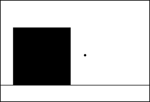
Figure 14-7. Simulating a falling ball to scale
First you need to choose the units for relevant physical quantities in your simulation. The most important units you need are those for time, length, and mass. They are called base quantities in physics. Other quantities, such as velocity and acceleration, depend on these base quantities, and their units can be derived from those of the base quantities by using their defining equations; they are therefore called derived quantities.
In this case, because mass drops out of the equations, it’s completely irrelevant what unit or indeed what value you use for the mass of the ball. So that leaves two base quantities we need to worry about: time and length (or distance).
Let’s assume that you want real-time simulation: in other words, the simulation should proceed at the same rate as real “wall-clock” time. (Sometimes you might not want this: for example, if you are simulating the solar system, you may not want to wait a year for the Earth to go around the Sun once!) In Figure 14-7, the ball in your simulation would then take exactly the same time to fall as it would if falling from the height of a real building. Therefore, you choose to measure time in seconds, as in real life. Not only that, but you want 1 second of simulation time to be equal to 1 second of real time: your scaling factor for time is 1.
The natural unit of distance to use for a screen-based visual simulation is the pixel (px). You also need to decide on an appropriate scaling factor to convert actual distances to pixels.
Scaling factors and parameter values
Suppose that the building in your scene would be 5 m tall in real life, and that you represent it by a rectangle of height 200 px. That means your scaling factor is 0.025 m/px; each pixel represents 0.025 m or 2.5 cm. You can use this length scale factor to scale other objects accordingly. So if your ball is a volleyball of radius 10 cm, its radius in the simulation would be 4 pixels.
Going back to our original question: what value should you give to g? The way you figure this out is as follows. Being an acceleration, g is measured in m/s2. Now, each second is an actual second in the simulation, but each meter is 40 px in the simulation. Therefore, scaling the approximate value of g = 10 m/s2 would give g = 400 in the simulation!
The file scale-model.jsimplements these values in this simple simulation. In the code, the ball is made to stop when it falls the 200 px (equivalent to 5 m in reality) to the ground. The time since the beginning of the simulation is then traced. Run the simulation and you’ll find that the ball takes approximately 1 second to fall to the ground. Is this realistic? It’s easy to find out using the old formula you met in Chapter 4:
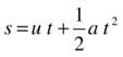
Here the displacement s is the height fallen (5 m), u is the initial velocity magnitude (zero), and a is the acceleration due to gravity g (10 m/s2). Substituting these values indeed gives t = 1 s. We have a real-time scale model! The value traced in the simulation is not exactly 1, but it is close enough. One of the reasons it’s not exactly 1 is that the ball is detected to be past the ground level slightly later because it’s moving so fast. When you run the simulation, you’ll see that it stops slightly below the “ground.”
Suppose you naively gave g the value of 10 in the simulation. What would be the consequence? Do this now, and you should find that the ball takes more than 6 seconds to reach the ground—hardly realistic!
Of course, you may not always need to be as careful as this in fixing the parameters of your simulation. You may not care about having a scale model at all; perhaps you are just interested in creating an animation that looks roughly right. But it’s useful to know how to do this when realism is really important. In more complex simulations it helps to have a systematic method to work out the values of your parameters.
The method of rescaling an equation is a formal procedure that can help to work out appropriate values for the parameters in your simulation. It is especially useful when you have more than one parameter whose value you need to work out or if there are multiple scale factors, but we’ll demonstrate the method for the simple example we’ve just looked at.
Rescaling involves scaling the variables in a system, re-expressing the equations in terms of the new scaled variables, and then comparing the scaled equation with the original one. The procedure is as follows.
First, write down the governing equation or equations (algebraic or differential), identifying all the variables. In our example, the equation is a = g, but this is really the following differential equation:

Next, define scaling factors for each of the variables as follows:
![]()
Here, the variables with hats are the new scaled variables, and the Greek letters are the corresponding scaling factors.
Then substitute the old variables into the original equation. In the preceding differential equation, note that the second derivative means that we are dividing a displacement increment by a time increment twice. Making the substitution, we therefore arrive at this:

We can rewrite this transformed equation as the following:

Comparing this with the original equation, we deduce that the equation in terms of the scaled variables will be exactly the same form as the original equation, provided that the right side is equal to the rescaled value of g:

This equation gives a constraint between the scaling factors and the rescaled value of the parameter g. So if we choose two of them, we can obtain the third. In this example, we chose the scaling factors for distance and time. So we can get the rescaled value of g by substituting the values of the scaling factors τ and λ. The scaling factor τ for time t is 1, as discussed previously, while the scaling factor λ for distance s is 5/200 or 0.025 m/px, as shown in the previous subsection. Therefore, the scaled value of g that we need for the simulation is given by the following:
![]()
This is just as we reasoned earlier.
Note that we could alternatively fix the rescaled value of g together with the scaling factor of one of the variables (either time or length). The previous constraint would then give us the scaling factor for the remaining variable.
For this simple example, the formal procedure just outlined is certainly overkill, but add in more variables and a more complex system of equations, and it will come in handy indeed.
Summary
If you plan to get into physics simulation seriously, sooner or later you need to worry about the accuracy and stability of your integration scheme. This chapter has presented some of the most common options at your disposal. The choice of a particular scheme depends on the problem as well as on other practical factors. In the previous chapters of the book we used the Euler scheme exclusively. In Chapter 16 you’ll see an example in which you need a more accurate integration scheme.