![]()
This final chapter consists of three simulation projects that will illustrate how the physics and methods you’ve learned in this book can be used for different types of applications. The examples are quite different from one another, reflecting differences not only in the underlying physics but also in the purposes for which they are built.
The three examples include the following:
- Building a submarine: The aim here is to show how easily you can modify some of the existing code you’ve already come across to create a submarine that you could incorporate in a 2D game.
- Building a flight simulator: In this example we’ll create a 3D flight simulator that could be further developed in many interesting ways just for pure fun!
- Creating an accurate solar system model: This project is to create an accurate 3D model of the solar system that could be used as an e-learning tool. We will then compare the simulation with data generated from a simulation by NASA.
The idea is that these are your projects, so we will describe the relevant physics and help you build a basic version, but then leave it to you to develop and enhance them in any ways you might want. Have fun!
Building a submarine
In Chapter 7 we had a simple but interesting example of a ball floating in water. It is actually quite easy to modify that example and turn it into an interactive submarine of a type that can be used in simple 2D games. Let’s first quickly review the main physics involved.
Brief review of the physics
In the floating-ball example, we identified three main forces that acted on the ball: gravity, upthrust, and drag, which are given respectively by the following formulas:
![]()
![]()
![]()
Note that we have written the upthrust formula in vector form: the minus sign is needed because upthrust acts upward, opposing the gravity vector g. Just as a reminder, in that formula ρ is the density of water and V is the volume of water displaced by the object.
With a submarine you have a fourth force: the thrust T that pushes the sub, allowing it to move horizontally through the water. This will be modeled as a horizontal force of constant magnitude when power is applied.
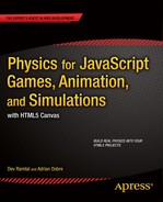
Another relevant piece of physics (as discussed in Chapter 7), is that an object will float if its density (mass per unit volume) is less than or equal to that of water, and it will sink otherwise. A submarine functions on the principle that its effective density can be varied by filling ballast tanks with sea water or pressurized air: its density (mass/volume ratio) varies because its mass thus changes while its volume remains the same.
The visual background is quite simple, consisting of a rectangle with a gradient fill to represent the sky and another one to represent the sea—both are created using the drawing API. A screenshot of the simulation is shown in Figure 16-1. There is also some text on the screen that displays the ratio of the density of the submarine to that of the water.
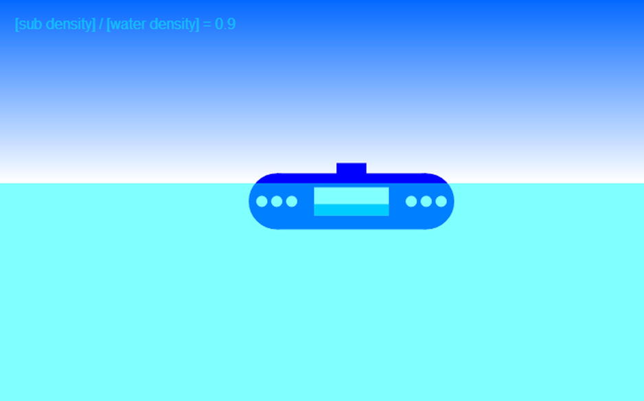
Figure 16-1. Screenshot of the submarine simulation
The submarine is created, using the drawing API, as a JavaScript object Sub—the code is in the file sub.js, available along with all of the source code and related files at www.apress.com. Figure 16-2 takes a closer look at it. The blue rectangle within the sub represents water in the ballast tanks. By controlling its height, we create the illusion of changing the water level, with the mass of the submarine being adjusted accordingly.

Figure 16-2. A closer look at the submarine
The setup code
The setup code is in the init() method of the simulation’s file submarine.js. The code in init() is listed here:
function init() {
     // create the sky
     gradient = context_bg.createLinearGradient(0,0,0,yLevel);
     gradient.addColorStop(0,'#0066ff');
     gradient.addColorStop(1,'#ffffff');
     context_bg.fillStyle = gradient;
     context_bg.fillRect(0,0,canvas_bg.width,yLevel);
     // create the sea
     context_fg.fillStyle = "rgba(0,255,255,0.5)";
     context_fg.fillRect(0,yLevel,canvas.width,canvas.height);
     // create a sub
     sub = new Sub(160,60,'#0000ff',emptySubMass);
     sub.pos2D = new Vector2D(250,300);
     sub.velo2D = new Vector2D(40,-20);
     sub.draw(context);
     // set water height in sub
     setWaterHeight();
     // set up text formatting
     setupText();
     // set up event listener
     window.addEventListener('keydown',keydownListener,false);
     // initialise time and animate
     initAnim();
}
Note that we are using three canvas instances (see the markup in the associated HTML file, submarine.html). The sky is drawn on a background canvas, and the sea is drawn on a foreground canvas. The sub is placed on a canvas instance in the middle. Naturally, the last two canvas elements are made transparent (see the associated style file, style7.css). The water level in the sub is set in the setWaterHeight() method, and the text formatting is set up in the setupText() method. A keydown event listener is then set up, and finally the initAnim() method, which initiates the animation code, is called.
The Sub object is created with four arguments, specifying its width, height, color, and mass, respectively. In addition to these properties it has a tankWidth and a tankHeight property, which are by default set to half of its width and height, respectively. It also has a waterHeight property, with a default value of 0. It has position (x and y) and velocity (vx and vy) properties, and associated pos2D and velo2D getters and setters. Finally, it has a draw() method, which draws the sub’s body, the tank, and the water level. See the code in sub.js.
The rest of the code is a modification of the floating simulation floating-ball.js that we created back in Chapter 7. The main changes have to do with the visual effects and controls (they are described in the next section). The basic motion code, as implemented in the calcForce() method, is not actually very different from that in floating-ball.js. Here is the calcForce() method:
function calcForce(){
     var rheight = 0.5*sub.height;
     var ysub = sub.y + rheight;
     var dr = (ysub-yLevel)/rheight;
     var ratio; // volume fraction of object that is submerged
     if (dr <= -1){ // object completely out of water
          ratio = 0;
     }else if (dr < 1){ // object partially in water
          ratio = 0.5+0.5*dr; // for cuboid
     }else{ // object completely in water
          ratio = 1;
     }
     var gravity = Forces.constantGravity(sub.mass,g);
     var upthrust = Forces.upthrust(rho,V*ratio,g);
     var drag = Forces.drag(k*ratio,sub.velo2D);
     force = Forces.add([gravity, upthrust, drag, thrust]);
}
The variable dr is the fraction of the height of the sub that is submerged under the water level. The variable ratio is the volume fraction that is submerged (which determines the upthrust and drag on the sub) and depends on the shape of the sub in a complex way. Because this simulation is meant for a simple game, it makes sense to deal with it in an approximate way. So we simply treat the sub like a cuboid, in which case the volume ratio is equal to 0.5 + 0.5*dr as long as the value of dr is between 0 and 1. If dr is negative (in which case the sub is completely outside the water), ratio is set to zero. If dr is greater than 1 (in which case the sub is fully immersed), ratio is set to 1.
The variable ratio is used to adjust the upthrust and drag, and they are then added to the weight of the sub. There is a fourth force, thrust, that is added and that obviously did not appear in the floating-ball example of Chapter 7. This is a Vector2D variable whose value is set according to user interaction. So let’s take a look at how the user controls the simulation.
Adding controls and visual effects
The aim is to control the submarine by means of the arrow keys on the keyboard. The right arrow will apply a forward thrust; the left arrow will apply a backward thrust; the down arrow will introduce water in the ballast tanks; and the up arrow will remove water from the ballast tanks and fill them with air. This is done via the following two event handlers, which respond to the keydown and keyup keyboard events, respectively:
function keydownListener(evt){
     if (evt.keyCode == 39) { // right arrow
          thrust = new Vector2D(thrustMag,0);
     } else if (evt.keyCode == 37) { // left arrow
          thrust = new Vector2D(-thrustMag,0);
     }
     if (evt.keyCode == 40) { // down arrow
          ballastInc = incMag;
     } else if (evt.keyCode == 38) { // up arrow
          ballastInc = -incMag;
     }
     window.addEventListener('keyup',keyupListener,false);
}
function keyupListener(evt){
     thrust = new Vector2D(0,0);
     ballastInc = 0;
     window.removeEventListener('keyup',keyupListener,false);
}
The variables thrustMag and incMag control the amount of thrust and the amount by which the water level is to be increased or decreased per timestep. The default values in the code are 20 and 0.01, respectively. The current values of thrust and water level increment are stored in the variables thrust and ballastInc, respectively. The thrust and water level increment are both reset to zero when the keys are up again.
The necessary visual changes are controlled by individual methods that are called at each timestep from the updateSub() method in the move() method:
function updateSub(){
     adjustBallast();
     updateInfo();
}
The adjustBallast() method increments the waterFraction variable, which keeps track of the amount of water in the ballast tank as a fraction of the amount when it is full. Obviously, that fraction cannot be made less than 0 or more than 1; hence the code also makes sure that never happens:
function adjustBallast(){
     if (ballastInc != 0){
          waterFraction += ballastInc;
          if (waterFraction < 0){
               waterFraction = 0;
          }
          if (waterFraction > 1){
               waterFraction = 1;
          }
          setWaterHeight();
     }
}
The final line of code in adjustBallast() calls a setWater() method, whose task it is to adjust the height of the water level and the mass of the sub as a result of the change in the mass of the water in the tank:
function setWaterHeight(){
     sub.waterHeight = sub.tankHeight*waterFraction;
     sub.mass = emptySubMass + waterMass*waterFraction;
}
The final method called from updateSub() is the updateInfo() method, which computes and displays the updated ratio of the density of the submarine to that of water:
function updateInfo(){
     var ratio = sub.mass/V/rho; // ratio of submarine density to water density
     ratio = Math.round(ratio*100)/100; // round to 2 d.p.
     var txt = "[sub density] / [water density] = ";
     txt = txt.concat(ratio.toString());
     context_fg.clearRect(0,0,700,100);
     context_fg.fillText(txt,20,20);
}
To show how everything fits together, we list here the full code of submarine.js:
var canvas = document.getElementById('canvas');
var context = canvas.getContext('2d');
var canvas_bg = document.getElementById('canvas_bg');
var context_bg = canvas_bg.getContext('2d');
var canvas_fg = document.getElementById('canvas_fg');
var context_fg = canvas_fg.getContext('2d');

var sub;
var g = 10;
var rho = 1;
var V = 1;
var k = 0.05;
var yLevel = 200;
var thrustMag = 20;
var thrust = new Vector2D(0,0);
var waterMass = 1;
var emptySubMass = 0.5;
var waterFraction = 0.4; // must be between 0 and 1
var ballastInc = 0; // ballast increment
var incMag = 0.01; // magnitude of the ballast increment
var t0, dt
var force, acc;
var animId;

window.onload = init;

function init() {
     // create the sky
     gradient = context_bg.createLinearGradient(0,0,0,yLevel);
     gradient.addColorStop(0,'#0066ff');
     gradient.addColorStop(1,'#ffffff');
     context_bg.fillStyle = gradient;
     context_bg.fillRect(0,0,canvas_bg.width,yLevel);
     // create the sea
     context_fg.fillStyle = "rgba(0,255,255,0.5)";
     context_fg.fillRect(0,yLevel,canvas.width,canvas.height);
     // create a sub
     sub = new Sub(160,60,'#0000ff',emptySubMass);
     sub.pos2D = new Vector2D(250,300);
     sub.velo2D = new Vector2D(40,-20);
     sub.draw(context);
     // set water height in sub
     setWaterHeight();
     // set up text formatting
     setupText();
     // set up event listener
     window.addEventListener('keydown',keydownListener,false);
     // initialize time and animate
     initAnim();
};
function setupText(){
     context_fg.font = "12pt Arial";
     context_fg.textAlign = "left";
     context_fg.textBaseline = "top";
}
function keydownListener(evt){
     if (evt.keyCode == 39) { // right arrow
          thrust = new Vector2D(thrustMag,0);
     } else if (evt.keyCode == 37) { // left arrow
          thrust = new Vector2D(-thrustMag,0);
     }
     if (evt.keyCode == 40) { // down arrow
          ballastInc = incMag;
     } else if (evt.keyCode == 38) { // up arrow
          ballastInc = -incMag;
     }
     window.addEventListener('keyup',keyupListener,false);
}
function keyupListener(evt){
     thrust = new Vector2D(0,0);
     ballastInc = 0;
     window.removeEventListener('keyup',keyupListener,false);
}

function initAnim(){
     t0 = new Date().getTime();
     animFrame();
}

function animFrame(){
     animId = requestAnimationFrame(animFrame,canvas);
     onTimer();
}
function onTimer(){
     var t1 = new Date().getTime();
     dt = 0.001*(t1-t0);
     t0 = t1;
     if (dt>0.2) {dt=0;};
     move();
}
function move(){
     updateSub();
     moveObject();
     calcForce();
     updateAccel();
     updateVelo();
}
function stop(){
     cancelAnimationFrame(animId);
}
function updateSub(){
     adjustBallast();
     updateInfo();
}
function adjustBallast(){
     if (ballastInc != 0){
          waterFraction += ballastInc;
          if (waterFraction < 0){
               waterFraction = 0;
          }
          if (waterFraction > 1){
               waterFraction = 1;
          }
          setWaterHeight();
     }
}
function setWaterHeight(){
     sub.waterHeight = sub.tankHeight*waterFraction;
     sub.mass = emptySubMass + waterMass*waterFraction;
}
function updateInfo(){
     var ratio = sub.mass/V/rho; // ratio of submarine density to water density
     ratio = Math.round(ratio*100)/100; // round to 2 d.p.
     var txt = "[sub density] / [water density] = ";
     txt = txt.concat(ratio.toString());
     context_fg.clearRect(0,0,700,100);
     context_fg.fillText(txt,20,20);
}
function moveObject(){
     sub.pos2D = sub.pos2D.addScaled(sub.velo2D,dt);
     context.clearRect(0, 0, canvas.width, canvas.height);
     sub.draw(context);
}
function calcForce(){
     var rheight = 0.5*sub.height;
     var ysub = sub.y + rheight;
     var dr = (ysub-yLevel)/rheight;
     var ratio; // volume fraction of object that is submerged
     if (dr <= -1){ // object completely out of water
          ratio = 0;
     }else if (dr < 1){ // object partially in water
          ratio = 0.5+0.5*dr; // for cuboid
     }else{ // object completely in water
          ratio = 1;
     }
     var gravity = Forces.constantGravity(sub.mass,g);
     var upthrust = Forces.upthrust(rho,V*ratio,g);
     var drag = Forces.drag(k*ratio,sub.velo2D);
     force = Forces.add([gravity, upthrust, drag, thrust]);
}
function updateAccel(){
     acc = force.multiply(1/sub.mass);
}
function updateVelo(){
     sub.velo2D = sub.velo2D.addScaled(acc,dt);
}
The submarine is now ready for a test drive! Have fun playing around and experimenting with the parameter values as you’ve done with examples throughout the book.
It’s your turn
That wasn’t too bad, was it? You now have a basic but functional submarine that you can add in a game. Now that it’s in your hands, you can further develop it as you see fit. You can enhance the visual appearance of the sub, add scenery such as a nice background with aquatic creatures and plants, add bubbles, and so on. You could add a sea floor and handle contact with it using a normal force. It should also not be very difficult to convert this simulation to 3D. If you do that, you would, of course, also need to include code to handle rotation.
Building a flight simulator
This project is quite a bit more complicated than the preceding example because we’ll be working in 3D, and also because the physics and operation of aircraft are fairly complex. Therefore, we’ll need to spend a bit more time on theory before we can get to the coding.
Physics and control mechanisms of aircraft
There are two aspects of theory to understand in order to simulate aircraft flight. The first is the underlying physics, which includes an understanding of the forces and torques acting on the aircraft and how they affect the aircraft’s motion. The second aspect is the mechanism by which aircraft control these forces and torques; this requires an understanding of the relevant parts of the aircraft and their associated maneuvers.
We discussed the forces that act on an airplane in Chapter 7: gravity, thrust, drag, and lift. Figure 16-3 shows a force diagram for a plane at an angle to the horizontal. This is a generalization of the force diagram shown in Figure 7-15, which was for the special case of an airplane in horizontal flight. Therefore, the directions of the thrust and drag are not necessarily horizontal, and the lift is not necessarily vertical. As a result, the force balance is a little more complex in this case. It is clearly important to get the magnitudes as well as the directions of these different forces right at all times (during ascent and descent, not just during horizontal flight), so we need robust equations for computing them in general.
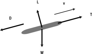
Figure 16-3. The four forces acting on an airplane during flight
The force of gravity W = mg still acts downward and is constant, of course; so that one is easy. The thrust T, whether generated by a propeller or by a jet engine, will usually act along the axis of the plane in the forward direction (unless you are considering an aircraft model such as the Harrier, in which the direction of the thrust can be varied). The magnitude of the thrust depends on many factors such as engine type, engine efficiency, and altitude effects. In our simulation, we’ll disregard all these effects, simply prescribing a value that can be changed by the user.
The drag and lift forces are more subtle. Strictly speaking, they are defined relative to the direction of the airflow over the relevant aircraft part such as the wing. Assuming there is no wind, we can approximate this as the direction of the aircraft’s velocity. The drag force can then be defined as the component of the aerodynamic force (force exerted as a result of the airflow) that acts opposite to the aircraft’s velocity. The lift force is the component perpendicular to the aircraft’s velocity.
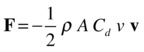
The drag formula is the same as that given in Chapter 7, in which v is now interpreted as the velocity of the aircraft:
The lift formula that we gave in Chapter 7 is generalized to the following formula, in which k is a unit vector perpendicular to the plane’s velocity and oriented to point upward from the plane’s wings:

These are general formulas that need to be adapted once we look at the aircraft parts in more detail. In particular, the relevant areas for use in those equations should be defined. We also need to specify the drag and lift coefficients, which can vary depending on several factors.
Torques on an aircraft: rotation
The forces on an aircraft are not sufficient to compute its motion. As you know, the resultant force determines the translational motion, but these forces can also exert torques if their lines of action do not pass through the center of mass. The weight of an object acts through a point known as its center of gravity. In uniform gravitational fields such as near the surface of the Earth (and an airplane is near enough the Earth’s surface for that purpose), the center of gravity coincides with the center of mass. Therefore, the weight of an airplane never generates a torque. However, the drag and lift forces act through a point known as the center of pressure. This is a similar concept to that of center of gravity, but it depends on the shape and inclination of the airplane, and does not in general coincide with its center of mass. So it can produce a torque that can send the aircraft spinning if unbalanced. An aircraft therefore needs to have stability mechanisms in place to balance this torque.
Of course, you do sometimes want an airplane to rotate. Figure 16-4 shows three ways in which an airplane can rotate about its center of mass and the axes about which it does so. It can pitch by moving its nose and tail up and down; it can roll by moving its wing tips up and down; and it can yaw by moving its nose and tail sideways. The axes are defined relative to the shape of the aircraft, and they all pass through its center of gravity. The pitch axis is oriented in a direction parallel to the wingspan, the roll axis is along the length of the aircraft, and the yaw axis is perpendicular to the other two axes. An aircraft is designed so that it has special parts that can produce these types of motion by controlling the lift and drag forces. Let’s look at those now.
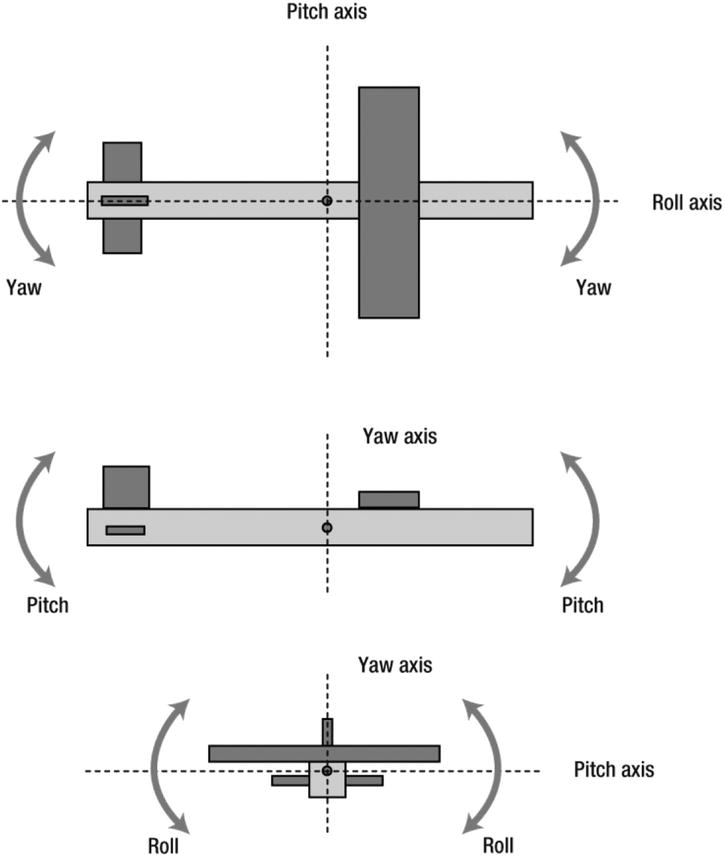
Figure 16-4. Pitch, roll, and yaw
Aircraft can control their motion by modifying the thrust, drag, and lift forces acting on them. This section briefly describes the parts of an aircraft that do this and how they do it. The thrust is controlled by the engine (which can be of different types, such as propeller or jet) and will propel the plane forward. Figure 16-5 shows a schematic of an airplane emphasizing those parts that are relevant to drag and lift and their control.
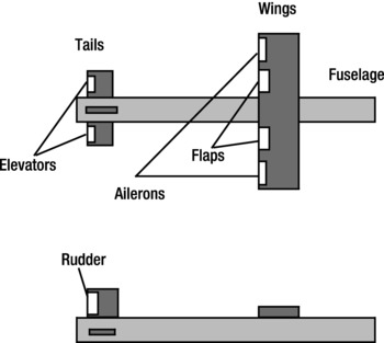
Figure 16-5. Aircraft parts
Fixed “main” parts include these:
- Fuselage: This is the main body of the aircraft. It is responsible for much of the drag. It also creates lift and pitching torque, but only for large angles of inclination, and they can usually be neglected. It can also create yawing torque for large lateral inclination; again this can usually be neglected.
- Wings: The two wings of an aircraft contribute most of the lift and drag forces on it. Without wings, an airplane just wouldn’t fly. The center of pressure of the lift and drag forces on the main wings is close to the center of mass, so one can assume that they contribute no torque, just like the fuselage. However, they have movable parts called flaps and ailerons that can be maneuvered to modify the lift and drag force and generate rolling torque.
- Tails: The tails consist of two parts: a horizontal and a vertical tail, which help in maintaining horizontal and vertical stability of the airplane. They also have movable parts called elevators and rudders that generate pitching and yawing torques.
Movable “control” parts include the following:
- Flaps: Flaps are attached to the rear of the wings and are rotated downward during takeoff and landing to increase the lift force (and also the drag force during landing to slow down the fast-moving aircraft).
- Ailerons: Ailerons are also attached to the rear of the wing, but farther along toward the wing tips. Rotating an aileron downward increases the lift, and rotating it upward decreases the lift. The two ailerons are rotated in opposite directions to produce a rolling torque (couple). Because the ailerons are far from the center of mass, large torques can be produced by relatively small changes in lift on either side of the wings (recall that moment = force × distance). Ailerons are usually controlled by a control stick; moving the stick to the right or left causes the aircraft to roll to the right or left.
- Elevators: Elevators are hinged to the rear side of the horizontal tail. Unlike ailerons, the elevators move together (both upward or both downward), thereby generating a pitching torque. Elevators are controlled by moving a stick forward to raise the nose of the aircraft and moving the stick backward to cause the aircraft nose to dip.
- Rudder: The rudder is attached to the rear of the vertical tail fin. It can rotate to either side, causing a yawing torque. The rudder is controlled by two foot pedals so that depressing the left or right pedal moves the aircraft’s nose to the left or right, respectively.
Airfoil geometry and angle of attack
The shape and inclination of aircraft wings are important factors that determine the magnitude of lift. Figure 16-6 shows the shape of a cross-section of a wing, called an airfoil. The shape of an airfoil is usually rounded at the front and sharp at the rear. The line joining the centers of curvature of the front and rear edges is called the chord line.
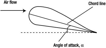
Figure 16-6. Flow over an aircraft wing (airfoil)
The angle between the chord line and the incident air flow (which is generally along the velocity of the plane) is called the angle of attack, usually denoted by the Greek letter α. The drag and lift coefficients of an airfoil depend on the angle of attack, and flight models generally use experimental data or a simple function to evaluate those coefficients as a function of angle of attack.
An airplane can take off only if its velocity exceeds a certain threshold. That threshold value corresponds to the point at which the lift force balances the weight of the plane. In that case, you can equate the expressions for the lift force and the weight:
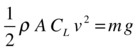
You can then rearrange this formula to give a formula for the velocity, which is the threshold velocity for takeoff:

During landing you have the opposite problem. You don’t want the velocity with which the plane touches the ground to be too high; otherwise, the plane will crash. You can set a reasonable threshold velocity in your game or simulation. Another consideration during landing is that the pitch angle must be zero or slightly positive; otherwise, the nose of the plane will hit the ground.
Turning is achieved by banking to give a horizontal unbalanced component of the lift force that, because it is always perpendicular to the velocity, generates a centripetal force that makes the plane move in a circle (see Figure 16-7). Banking is achieved by rolling the plane using the ailerons. The yawing motion produced by a rudder is not used for turning, but for aligning the plane in the direction of the velocity.
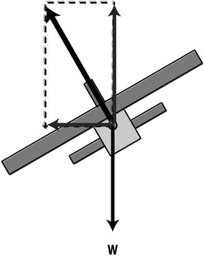
Figure 16-7. Force diagram for a banked plane
What we will create
The simulation we will create will include the essential physics needed to make an airplane fly, with the ability to undergo the different types of motion (straight flight, pitch, roll, and yaw) and maneuvers (takeoff, landing, and turning) discussed. The user will be able to control a very simple airplane model using the keyboard, in a similar way to a pilot controlling an airplane. The operation of the elevators, ailerons, and rudder in creating pitching, rolling, and yawing torque will be simulated. The user can also adjust the amount of thrust. For simplicity we won’t include flaps—however, they can easily be added.
The visual setup is minimalist, consisting of just the ground and a very simple airplane model represented with a cuboid. The code is in the file airplane.js and the init() method looks like this:
function init() {
     setupObjects();
     setupOrientation();
     setupText();
     renderer.render(scene,camera);
     window.addEventListener('keydown',startControl,false);
     t0 = new Date().getTime();
     animFrame();
}
The first two methods setupObjects() and setupOrientation() are responsible for creating the display objects and initializing the airplane’s orientation respectively. Let’s look at setupObjects() first:
function setupObjects(){
     renderer = new THREE.WebGLRenderer({clearColor: 0xff0000, clearAlpha: 1});
     renderer.setClearColor( 0x82caff, 1);
     renderer.setSize(width, height);
     document.body.appendChild(renderer.domElement);

     scene = new THREE.Scene();

     var angle = 45, aspect = width/height, near = 0.1, far = 10000;
     camera = new THREE.PerspectiveCamera(angle, aspect, near, far);
     camera.position.set(100,0,1000);
     scene.add(camera);

     var light = new THREE.DirectionalLight();
     light.position.set(30,0,30);
     scene.add(light);

     var geom = new THREE.PlaneGeometry(5000, 100000, 50, 500);
     var wireframeMat = new THREE.MeshBasicMaterial();
     wireframeMat.wireframe = true;
     var ground = new THREE.Mesh(geom, wireframeMat);
     ground.rotation.x = -Math.PI/2;
     ground.position.set(0,groundLevel,0);
     scene.add(ground);

     airplane = new THREE.Mesh(new THREE.CubeGeometry(400, 100, 100), new THREE.MeshNormalMaterial());
     airplane.overdraw = true;
     scene.add(airplane);
     airplane.mass = massAirplane;
     airplane.pos = new Vector3D(0,200,0);
     airplane.velo = new Vector3D(0,0,0);
     airplane.angVelo = new Vector3D(0,0,0);
}
The “ground” is created using PlaneGeometry with MeshBasicMaterial and a wireframe option, and is rotated around the x-axis by 90 degrees. The airplane is created using CubeGeometry and is given a mass, a position vector, a velocity vector, and an angular velocity. The moment of inertia of the airplane is specified in the variable I, which is initialized in the list of variables at the beginning of the code. As discussed in the previous chapter, the moment of inertia is a 3 × 3 matrix in 3D. Here we consider the inertia matrix to consist of only three diagonal components: Ixx, Iyy, and Izz, the other components of the matrix being taken to be zero. In order to implement the required matrix algebra (see the following section on “Coding up the physics”) we have coded a very simple Matrix3D object that creates a 3 × 3 matrix by considering each row of the matrix as a Vector3D object. Matrix3D therefore takes three Vector3D arguments in its constructor. We have endowed Matrix3D with two methods, multiply() and scaleBy(), which multiply it with a Vector3D object and a scalar, respectively. See the code in the file matrix3D.js for the detailed implementation.
Note that the airplane is created such that it is initially oriented with its length along the x-axis. In the simulation, we’ll want it to point along the –z-axis so that it flies into the screen. To achieve this, the setupOrientation() method rotates the plane by 90 degrees about the y-axis:
function setupOrientation(){
     // initialize airplane orientation
     var qRotate = new THREE.Quaternion();
     qRotate.setFromAxisAngle(new THREE.Vector3( 0, 1, 0 ), Math.PI/2);
     airplane.quaternion.multiply(qRotate);

     // airplane local axes
     ix = new Vector3D(1,0,0);
     iy = new Vector3D(0,1,0);
     iz = new Vector3D(0,0,1);
}
We also define three vectors ix, iy, and iz to represent the airplane’s three axes in its own frame of reference. These will be needed for calculating the lift forces and torques on the airplane in calcForce(). Referring to Figure 16-4, these axes correspond to the roll, yaw and pitch axes respectively. They are defined relative to the airplane, and will therefore change relative to the ground, in so-called “world frame.”
Coding up the physics
The animation loop is set up by a call to the animFrame() method in init(). This produces calls to familiar methods such as moveObject(), calcForce(), updateAccel(), and updateVelo(), which handle the updating of both the translational and rotational motion of the airplane as in previous examples. In addition there is a controlRotation() method that applies a bit of a hack to impose stability on the airplane’s rotational motion, preventing it from spinning out of control. In reality, the stability mechanism is quite complex, and would be rather difficult to implement properly. So we cheat a little in controlRotation(), simply applying a damping factor to the plane’s angular velocity.
The guts of the code consist of the calculation of the forces and torques on the airplane, which is done in the calcForce() method. This looks quite complicated at first sight, but it will make sense when you go through it step by step. We have also included plenty of comments in the downloadable source file; some of them are included in the following listings. Let us list the whole of calcForce() before discussing it:
function calcForce(obj){
     // *** rotate airplane velocity vector to airplane's frame ***
     var q = new THREE.Quaternion;
     q.copy(airplane.quaternion);
     var rvelo = rotateVector(obj.velo,q);

     // *** forces on whole plane ***
     force = new Vector3D(0,0,0);
     var drag = Forces3D.drag(kDrag,rvelo);
     force = force.add(drag);
     var thrust = new Vector3D(-thrustMag,0,0); // thrust is assumed along roll axis
     force = force.add(thrust);

     // *** torques on whole plane ***
     torque = new Vector3D(0,0,0); // gravity, drag and thrust don't have torques

     // *** lift forces and torques on wings and control surfaces ***
     if (rvelo.length() > 0){ // no lift if velocity is zero
          var viXY = new Vector3D(rvelo.x,rvelo.y,0); // velocity in the airplane xy plane
          var viZX = new Vector3D(rvelo.x,0,rvelo.z); // velocity in the airplane xz plane

          // *** calculate angle of attack and lateral angle ***
          calcAlphaBeta(rvelo);

          // *** Wing ***
          // force: lift on the Wing; no overall torque
          var liftW = liftforce(viXY,iz,areaWing,clift(alphaWing+alpha));
          force = force.add(liftW);

          // *** Ailerons ***
          // force: ailerons; form a couple, so no net force
          var liftAl = liftforce(viXY,iz,areaAileron,clift(alphaAl));
          var torqueAl = (iz.multiply(distAlToCM*2)).crossProduct(liftAl); // T = r x F
          torque = torque.add(torqueAl);

          // *** Elevators ***
          // force: horizontal tail (elevators)
          var liftEl = liftforce(viXY,iz,areaElevator,clift(alphaEl));
          torqueEl = (ix.multiply(-distTlToCM)).crossProduct(liftEl);  // T = r x liftHt;
          force = force.add(liftEl);
          torque = torque.add(torqueEl);

          // *** Rudder ***
          // force: vertical tail (rudder)
          var liftRd = liftforce(viZX,iy.multiply(-1),areaRudder,clift(alphaRd+beta));
          torqueRd = (ix.multiply(-distTlToCM)).crossProduct(liftRd); // T = r x liftVt
          force = force.add(liftRd);
          torque = torque.add(torqueRd);
     }

     // *** rotate force back to world frame ***
     force = rotateVector(force,q.conjugate());

     // *** add gravity ***
     var gravity = Forces3D.constantGravity(massAirplane,g);
     force = force.add(gravity);
}
A key feature of this simulation is that most of the force and moment calculations are performed in the airplane’s frame of reference. So we begin by rotating the airplane’s velocity vector into the airplane’s frame by applying the rotateVector() method, which makes use of the applyQuaternion() method in three.js. The drag force is then computed as opposite to this rotated velocity vector. The drag force is computed assuming a constant drag coefficient. This is a simplification; generally, the drag coefficient will depend on the angle of attack, but this dependence is not modeled here for simplicity. The thrust is applied in the direction of the plane’s ix (roll) axis, and its magnitude is controlled by the user by updating the thrustMag variable (as will be described later). The net torque due to these forces is assumed to be zero so that the plane maintains rotational equilibrium.
The next section of code computes the lift forces on the various surfaces of the airplane (wings, ailerons, elevators and rudder) and the moments produced by these forces. Because the lift force is zero if the plane is not moving, the whole calculation is only done if the plane’s velocity is non-zero. The lift forces consist of vertical lift on the wings, elevators, and ailerons and of horizontal lift on the rudder. They depend on the velocities in the xy and xz planes relative to the airplane. These velocities are therefore calculated first. Then they are used to compute the angle of attack α and lateral angle β (the angle between the x and z components of the plane’s velocity) in the calcAlphaBeta() function. Note that we are here assuming that there is no wind. It would be straightforward to add in the effect of the wind, but that would only complicate the code further.
Next, the lift force on the wings is calculated. The cross product is used because the lift force on the wings is perpendicular to the velocity in the xy plane and the wing axis (the pitch axis). The lift coefficient is calculated assuming a linear dependence on the angle of attack, with a constant gradient dCL/dα:
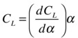
Note that we add the inclination of the wing relative to the plane’s roll axis (alphWing) to the value of α calculated previously to obtain the actual angle of attack. We also impose a limiting value on the lift force because in reality the lift force does not increase indefinitely with the angle of attack, but reaches a maximum value. The lift coefficient is calculated in the clift() function and the lift force in liftforce().
The lift force on the main wings is assumed to generate no torque when the plane is in equilibrium, just like drag and thrust (or, more accurately, the combined torques of these forces are made to cancel out in practice).
The next blocks of code compute the lift forces on the movable control surfaces (elevators, ailerons, and rudder) and the torques they generate. The lift calculation is done in the same way as for the main wings. The torques are calculated as usual by taking the cross product of the distance vector of the lift force from the center of mass and the lift force:
![]()
The appropriate distance vector needs to be specified for each control surface.
After all the lift forces are added to the force vector, the latter is then rotated back to the world frame and the gravity is added as a constant downward force. The subsequent calculation of the acceleration and velocity updates are then performed in the world frame as usual.
Note that the angular motion calculation is done in the airplane’s frame throughout the code. Here we have to be a little careful in how we apply the angular equation of motion (that is, the relationship between torque and angular acceleration). Because the airplane is in a rotating frame of reference, the latter has an additional term, and looks like this (see the section “Torque, angular acceleration, and the moment of inertia matrix” in Chapter 15):
![]()
Recall that this is a matrix equation, with the moment of inertia I being a 3 × 3 matrix and the torque T, angular velocity ω, and angular acceleration α = dω/dt being vectors. This equation can be easily manipulated to give a matrix equation for the angular acceleration:
![]()
Here ![]() is the inverse of the moment of inertia matrix. This equation can be discretized using a forward scheme and implemented in code as shown in the bold lines in the following listing of the updateAccel() method:
is the inverse of the moment of inertia matrix. This equation can be discretized using a forward scheme and implemented in code as shown in the bold lines in the following listing of the updateAccel() method:
function updateAccel(obj){
     acc = force.multiply(1/obj.mass);
     var omega = obj.angVelo;
     alp = Iinv.multiply(torque.subtract(omega.crossProduct(I.multiply(omega))));
}
The inverse moment of inertia matrix Iinv is precomputed in the code from the specified components of the moment of inertia matrix I.
Finally, the airplane’s orientation and position are updated in moveObject():
function moveObject(obj){
     var p = new THREE.Quaternion;
     p.set(obj.angVelo.x*dt/2,obj.angVelo.y*dt/2,obj.angVelo.z*dt/2,1);
     obj.quaternion.multiply(p);
     obj.quaternion.normalize();
     obj.pos = obj.pos.addScaled(obj.velo,dt);
     positionObject(obj);
     positionCamera(obj);
     renderer.render(scene,camera);
}
Note also the addition of the new positionCamera() method in moveObject(), which controls the camera position and movement, and which you are welcome to customize.
In the init() method an event listener is set up for keydown events. The airplane is controlled by using the arrow, X, and Z keys to control the elevators, ailerons, and rudder; and the spacebar and Enter key to control the thrust. This is done in the startControl() event listener. (We won’t list the code here because it’s quite straightforward.) The down-arrow key increases the pitch, raising the airplane’s nose upward, and the up key lowers it. The left- and right-arrow keys make the plane roll to the left and right, respectively. These movements are similar to the way the control stick is used by a pilot to control the elevators and ailerons. The rudder is controlled using the X and Z keys. The maximum angles and increments for these movable parts are set at the beginning of the program. The thrust magnitude is increased and decreased by pressing the spacebar and Enter keys, respectively. Again, the maximum magnitude of the thrust and its increment are set at the beginning of the code.
The camera position is controlled by pressing the A key to follow the airplane or the W key to remain at a fixed point in the world frame. Finally, pressing the Esc key stops the simulation.
Displaying flight information
The updateInfo() method, called at each timestep from the onTimer() method, contains code to write text on a separate canvas element as the simulation progresses. Information is displayed about the airplane’s altitude, vertical velocity, and horizontal velocity as well as the aileron, elevator, and rudder angles. The first two pieces of information are important to bear in mind when you are trying to keep the plane in flight without crashing it. A positive vertical velocity means that the plane is rising; if the vertical velocity is negative, it is losing altitude, so you better watch out.
You can easily add additional information such as the current position of the airplane (useful if you want to go somewhere).
The airplane is now ready to fly! Run it with the default parameter values. When the simulation starts, the plane will have an initial velocity of zero, but there is an applied thrust. If you don’t do anything, the airplane will initially fall under gravity, and then start rising as the applied thrust increases its horizontal velocity and hence provides lift. Increase the thrust by pressing and holding down the spacebar. Then increase the elevators’ angle by pressing the down-arrow key. You will see the plane gradually rising as it moves forward. Then decrease the pitch angle by pressing the up-arrow key, which will reduce the lift and decrease the ascent of the plane, or even make it descend. See if you can make the airplane rise up to a given altitude and remain there. To do that you need to play with the thrust and/or the pitch angle, and you need to make the vertical velocity reach close to zero at your desired altitude. Once you’ve achieved that, you can sit back and relax; the plane will take care of itself.
Restart the simulation and try out the aileron and rudder controls. Note that the plane turns when the plane rolls, just as described in the “Turning” section. Too much rolling or yawing might make the airplane behave somewhat unpredictably, though. See also the detailed comments included in the source code. Figure 16-8 shows a screenshot of the simulation with the plane in flight.

Figure 16-8. The airplane in flight
It’s your turn
You probably already have several ideas about how to improve this simulator. Creating a much more impressive 3D model airplane is probably one of them, and possibly more visually appealing scenery, too. You could go much further with the 3D effects, and also incorporate a more extensive terrain, which could be either generated or based on real aerial information. You could also improve the control of the airplane by adding flaps, include visual elements in the model to represent the control surfaces, add crash scenarios, and so on. You probably have even better ideas of your own!
Creating an accurate solar system model
This project will be somewhat different from most of the examples in the book. The aim here is to create an accurate computer model of the solar system that could be used as an e-learning tool for students. The key word here is accurate: the visual and animation effects are less important than the correctness of the physics and the accuracy of the simulation. Consequently, we will depart from our usual animation framework and adopt a somewhat different coding approach from the outset that will reflect the simulation rather than the animation aspect of the project.
What we will create
Our aim is to create a scale model of the solar system that includes the Sun and the planets. In the supplied source code we include the innermost four planets (Mercury, Venus, Earth, and Mars)—the so-called terrestrial planets. We leave it as an exercise for you to add the other four (Jupiter, Saturn, Uranus and Neptune)—the so-called gas giants. This should be easy to do, and will give you valuable hands-on experience with the code.
Note that Pluto is no longer classified as a planet. In the simulation we’ll pretend that smaller celestial bodies like these do not exist, including asteroids and moons. We can omit them because their effects on the motion of the planets are pretty negligible.
The project will proceed in different stages:
- Step 1: First, we’ll set up a simulation loop using the fourth-order Runge-Kutta scheme (RK4, introduced in Chapter 14) in 3D, which we’ll test with a simple example. The source code for this is in the file rk4test3d.js.
- Step 2: Second, we’ll use that simulation loop to model the motion of a single planet in a simple idealized way. The source code for that step is in the file single-planet.js.
- Step 3: Third, we will include the four inner planets and set their properties and initial conditions based on mean astronomical data, so that we’ll end up with a reasonably realistic solar system model (or rather half of it). We’ll also need to set up appropriate scales carefully. The corresponding file is named solar-system-basic.js.
- Step 4: Fourth, in the file solar-system.js, we will include accurate initial conditions and run the simulation for a year.
- Step 5: Fifth, in solar-system-nasa.js we’ll compare the results with corresponding simulation data from NASA to see how good our simulation is.
- Step 6: Finally, in solar-system-animated.js, we’ll introduce some basic animation to make the simulation more visually appealing.
The physics
The simulation will involve modeling the motion of each planet under the action of the combined gravitational force exerted on it by the Sun and the other planets. The effect of the Sun will, of course, be much larger because of its very large mass compared with those of any of the planets. We’ll adopt a coordinate system in which the Sun is fixed, so that we don’t have to model the motion of the Sun itself. The planets will be able to move in 3D space under the action of those forces.
Let m be the mass of a planet, ri its position vector relative to each of the other planets and the Sun (with riu being the corresponding unit vector), and mi the mass of each of the other planets and the Sun. Then the total force on each planet is given by the following formula:
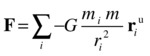
Dividing by the mass, we obtain the acceleration of each planet:
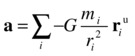
This is the equation that the numerical integration code will solve. That’s it. The physics of this problem is pretty simple! But there are other issues that make the simulation nontrivial: implementing an accurate numerical integration scheme, scaling the model properly, and incorporating accurate initial conditions. We’ll handle each of these requirements one step at a time.
Coding up an appropriate integration scheme
Because accuracy is our prime concern, it makes complete sense to use the RK4 integration method. To implement RK4, we’ll first create a simple “simulation loop” that will do the timestepping, but we’ll do that independently of the “animation loop” that we’ve been using so far. It’s easier to do this than to explain it, so let’s just do it and we’ll explain afterward.
We borrow the RK4 code from the examples in Chapter 14 and modify it to come up with the following code, which is in the file rk4test3d.js:
var dt = 0.05;
var numSteps = 20;
var t = 0;
var g = 10;
var v = new Vector3D(0,0,0);
var s = new Vector3D(0,0,0);

window.onload = init;

function init(){
     simulate();
}
function simulate(){
     console.log(t,s.y);
     for (var i=0; i<numSteps; i++){
          t += dt;
          RK4();
          console.log(t,s.y);
     }
}
function RK4(){
     // step 1
     var pos1 = s;
     var vel1 = v;
     var acc1 = getAcc(pos1,vel1);
     // step 2
     var pos2 = pos1.addScaled(vel1,dt/2);
     var vel2 = vel1.addScaled(acc1,dt/2);
     var acc2 = getAcc(pos2,vel2);
     // step 3
     var pos3 = pos1.addScaled(vel2,dt/2);
     var vel3 = vel1.addScaled(acc2,dt/2);
     var acc3 = getAcc(pos3,vel3);
     // step 4
     var pos4 = pos1.addScaled(vel3,dt);
     var vel4 = vel1.addScaled(acc3,dt);
     var acc4 = getAcc(pos4,vel4);
     // sum vel and acc
     var velsum = vel1.addScaled(vel2,2).addScaled(vel3,2).addScaled(vel4,1);
     var accsum = acc1.addScaled(acc2,2).addScaled(acc3,2).addScaled(acc4,1);
     // update pos and velo
     s = pos1.addScaled(velsum,dt/6);
     v = vel1.addScaled(accsum,dt/6);
     //acc = accsum.multiply(1/6);
}
function getAcc(ppos,pvel){
     return new Vector3D(0,g,0);
}
Okay, let’s start with the familiar. As stated earlier, the RK4() method is a modification of the RK4() method that we first saw in Chapter 14. If you compare the two versions, you will notice one crucial difference: this code deals with the current position and velocity through abstract variables s and v, instead of actual particle position and velocity properties as before. This is the first sign of the separation of the animation aspect from the simulation.
The getAcc() method that previously invoked calcForce() has been simplified here to simply return a constant acceleration vector pointing downward in the y direction. That means here we are specializing the code to a simple gravity problem. The other remaining piece of code is the simulate() method, which is called once upon initialization. The core of the code is incredibly simple. It is the following for loop that does all the timestepping, incrementing the current time and calling the RK4() method, which updates the position and velocity vectors s and v at each timestep:
for (var i=0; i<numSteps; i++){
     t += dt;
     RK4();
}
From an animation perspective, this code and the associated timestepping will execute all in one go: effectively we’ll be precomputing the motion before doing any animation of existing display objects. There isn’t even a display object in this code. The advantage of doing this is that it “decouples” the simulation loop from the animation loop (if there’s going to be one), so that either can do its job unhindered by any time delays introduced by the other. However, this approach doesn’t work if your simulation needs to be interactive.
Looking at how the variables are initialized, we can see that we are simulating the fall of an object from rest (v is initially zero) under gravity for one time unit (because dt * numSteps = 0.05 × 20 = 1). For example, choosing units of seconds for dt and m/s2 for g, this corresponds to letting an object fall from rest for 1 second under gravity with g equal to 10 m/s2. Using the formula s = ut + ½ at2 then tells us that the object falls a distance of 5 m in that time. In the code, we output to the console the pair of values t and s.y at each timestep, which tells us how far the object has fallen at each time. Run the code and you’ll find that the final distance is indeed 5. You can try different timesteps (adjusting the number of steps accordingly) and you’ll find that RK4 is doing a pretty good job, pretty much whatever the timestep. For example, even with a timestep of 0.5 and with 2 steps (so that the duration is still 1 time unit), it still gives exactly 5!
Now that we’ve got a good integrator and a basic simulation loop set up, we’re ready to move on and create something closer to a planetary system.
Building an idealized single-planet simulation
It is straightforward to modify the basic RK4 simulator we just created to simulate a planetary orbit: you essentially have to modify the getAcc() method according to Newton’s 1/r2 formula for gravitational force and choose appropriate initial conditions for s and v. But we also want to see something on the canvas! So, with a little help from three.js, we also add a sun and a planet using sphereGeometry, and include some code that will show us how their positions change with time. The result is the following code, saved as single-planet.js:
var width = window.innerWidth, height = window.innerHeight;
var dt = 0.05;
var numSteps = 2500;
var animFreq = 40;
var t = 0;
var v = new Vector3D(5,0,14);
var s = new Vector3D(0,250,0);
var center = new Vector3D(0,0,0);
var G = 10;
var massSun = 5000;
var scene, camera, renderer;
var sun, planet;

window.onload = init;

function init(){
     setupObjects();
     simulate();
     renderer.render(scene, camera);
}
function setupObjects(){
     renderer = new THREE.WebGLRenderer();
     renderer.setSize(width, height);
     document.body.appendChild(renderer.domElement);

     scene = new THREE.Scene();

     var angle = 45, aspect = width/height, near = 0.1, far = 10000;
     camera = new THREE.PerspectiveCamera(angle, aspect, near, far);
     camera.position.set(0,0,1000);
     scene.add(camera);

     var light = new THREE.DirectionalLight();
     light.position.set(-10,0,20);
     scene.add(light);

     var radius = 80, segments = 20, rings = 20;
     var sphereGeometry = new THREE.SphereGeometry(radius,segments,rings);
     var sphereMaterial = new THREE.MeshLambertMaterial({color: 0xffff00});
     sun = new THREE.Mesh(sphereGeometry,sphereMaterial);
     scene.add(sun);
     sun.mass = massSun;
     sun.pos = center;
     positionObject(sun);

     var sphereGeometry = new THREE.SphereGeometry(radius/10,segments,rings);
     var sphereMaterial = new THREE.MeshLambertMaterial({color: 0x0099ff});
     planet = new THREE.Mesh(sphereGeometry,sphereMaterial);
     scene.add(planet);
     planet.mass = 1;
     planet.pos = s;
     positionObject(planet);
}
function positionObject(obj){
     obj.position.set(obj.pos.x,obj.pos.y,obj.pos.z);
}
function simulate(){
     for (var i=0; i<numSteps; i++){
          t += dt;
          RK4();
          if (i%animFreq==0){
               clonePlanet(planet);
          }
     }
}
function clonePlanet(){
     var p = planet.clone();
     scene.add(p);
     p.pos = s;
     positionObject(p);
}
function getAcc(ppos,pvel){
     var r = ppos.subtract(center);
     return r.multiply(-G*massSun/(r.lengthSquared()*r.length()));
}
function RK4(){
     //code as in previous example
}
The first novel piece of code is in the setupObjects() method, which implements the three.js functionality and creates the sun and planets. Note that the rendering is done just once, at the end in the init() method, after setupObjects() and simulate() have executed. We have added an if block of code in the simulate() function that calls a clonePlanet() method at intervals of animFreq. The clonePlanet() method creates a copy of the planet and places it at the new position. The net result is a series of cloned planets at locations where the planet has been after equal amounts of time (see Figure 16-9). Not quite “animation,” because if you run the code you will see everything displayed at once, but it does convey some sense of stepping through time. This is a planetary trajectory in 3D; you can see the perspective effect causing the planet to appear smaller when its z-coordinate is greater. In terms of the physics, the most significant modification is that the getAcc() method now applies an acceleration due to the sun’s attraction on the planet. This produces the orbit that we see in Figure 16-9.
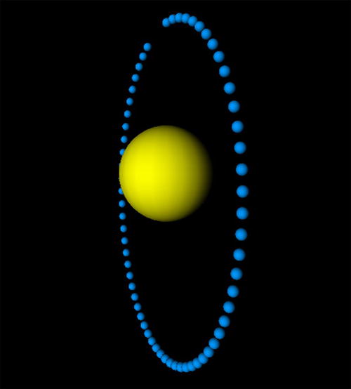
Figure 16-9. A planetary trajectory in 3D
Choosing appropriate scaling factors
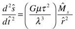
Now that we have an accurate orbit simulator, it’s time to represent the real solar system to scale as the next step toward a realistic simulation. To do this, we need to go back to the governing equation. For the purpose of choosing appropriate scaling factors, it is the form of the equation that matters instead of the details of the various terms. So it will be fine to consider only the portion of the equation reflecting the effect of the sun. Also, it’s the magnitude of the relevant quantities that matters, not their direction. The last equation therefore leads to the following approximate equation for the acceleration of each planet, in which Ms is the mass of the Sun and r is the distance of the planet from it:

We now define scaling factors for time, distance, and mass in a similar way to the example in the previous chapter:
![]()
Substituting these factors into the previous equation and rearranging gives the following corresponding equation in terms of the rescaled variables:
Comparing the two equations then tells us that the value of the gravitational constant G in the rescaled system is given by this:

We now need to choose appropriate scaling factors μ, τ, and λ for the base units for converting quantities from the usual SI units to corresponding simulation units. In any given problem a sensible choice for the scaling factors should reflect scales relevant to the physics. In this case, for example, it makes no sense to think of mass values in terms of kg but instead in terms of the mass of the Sun or the mass of the Earth. Let’s choose the latter. Similarly, it makes little sense to stick with the second as a unit of time, because we will be interested in seeing the planets complete at least one revolution around the Sun (the duration of the simulation will be on the order of years). Therefore, we’ll choose 1 day as the unit of time. Finally, we could choose the mean distance of the Earth from the Sun (known as an astronomical unit or au) as the distance unit. That’s about 150 million km, or 150 × 109 m. This would make the distance between the Earth and the Sun 1 unit in the simulation by definition. However, because we are building a visual simulation, we’ll be thinking of distance in terms of pixels and want to see the Earth a decent number of pixels away from the Sun. A more suitable choice of scaling factor in that case is 1 million km (109 m) per pixel, which would make the Earth-Sun distance around 150 pixels. Table 16-1 summarizes these choices of scaling factors.
Table 16-1. Scaling Factors for Base Units
Scaling factor |
Value |
|---|---|
μ (mass) |
Earth mass = 5.9736 x 1024 kg |
τ (time) |
Earth day = 86400 s |
λ (length) |
1 million km = 109 m |
Scaling factors for derived quantities such as velocity can be worked out from those of the base quantities. For example, the scale factor for velocity is given by λ/τ.
Obtaining planetary data and initial conditions
Next we need to obtain some planetary data such as the masses of the planets and some suitable values for the initial conditions (planets’ positions and velocities). This web page from NASA’s web site has all the required information: http://nssdc.gsfc.nasa.gov/planetary/planetfact.html.
For easy access, we have saved some of the data that we’ll be using as static constants in the Astro object. This includes, for example, the constants EARTH_MASS, EARTH_RADIUS, EARTH_ORBITAL_RADIUS, and EARTH_ORBITAL_VELOCITY and similar constants for other planets. Take a look at the file astro.js. There is a related class called Phys, in the file phys.js, which contains values of a few physical constants such as the gravitational constant G (GRAVITATIONAL_CONSTANT) and the standard value of the acceleration due to gravity on Earth (STANDARD_GRAVITY). These values were obtained from the following web page on the NIST web site: http://physics.nist.gov/cuu/Constants/.
The values of the mean orbital radius and the orbital velocity of the planets in the Astro object will be used as approximate initial conditions in the basic version of the solar system model that we will construct next.
Creating a basic solar system model
We are now ready to put together a basic solar system model that will include all the essential aspects of the simulation. The relevant file, solar-system-basic.js, contains a fair amount of code. So we’ll break it down a bit. Let’s begin by listing the variables and the init() method:
// rendering
var width = window.innerWidth, height = window.innerHeight;
var scene, camera, renderer;

// time-keeping variables
var dt = 1/24; // simulation time unit is 1 day; time-step is 1 hr
var numSteps = 8760; // 1 year; 365*24
var animFreq = 168; // once per week; 24*7
var t = 0;

// gravitational constant
var G;

// sun variables
var center;
var massSun;
var radiusSun = 30;

// arrays to hold velocity and position vectors for all planets
var v;
var s;

// visual objects
var sun;
var planets;
var numPlanets = 4;

// planets' properties
var colors;
var radiuses;
var masses;
var distances;
var velos;

// scaling factors
var scaleTime;
var scaleDist;
var scaleMass;
var scaleVelo;

window.onload = init;

function init(){
     setupScaling();
     setupPlanetData();
     setInitialConditions();
     setupObjects();
     simulate();
     renderer.render(scene, camera);
}
First, take a look at the variable definitions. Note in particular that s and v are now arrays that will hold the Vector3D positions and velocities of the planets. Note also the arrays colors, radiuses, and so on that will hold the properties of the planets. Next take a look at the init() function. The following methods are called in succession before the final rendering: setupScaling(), setupPlanetData(), setInitialConditions(), setupObjects(), and simulate(). Let’s briefly discuss each one in turn.
The setupScaling() method does exactly what its name suggests: it defines the scale factors and then uses them to rescale the mass of the sun and the gravitational constant to their simulation values:
function setupScaling(){
     scaleMass = Astro.EARTH_MASS;
     scaleTime = Astro.EARTH_DAY;
     scaleDist = 1e9; // 1 million km or 1 billion meters
     scaleVelo = scaleDist/scaleTime; // million km per day

     massSun = Astro.SUN_MASS/scaleMass;

     G = Phys.GRAVITATIONAL_CONSTANT;
     G *= scaleMass*scaleTime*scaleTime/(scaleDist*scaleDist*scaleDist);
}
The setupPlanetData() method puts the appropriate values for the planets’ properties in the five arrays radiuses, colors, masses, distances, and velos. The values we chose for radiuses are in proportion to the four planets’ real radii. But please note that they are not in proportion to the radius of the Sun (which in reality would be much larger compared with those of the planets). Moreover, neither the radii of the planets nor the radius of the Sun are in proportion to the distances between them. If we did that, the planets would all be tiny dots in the space available in the browser window. The masses, distances, and velocities are scaled values of those read in from the Astro object for each planet.
function setupPlanetData(){
     radiuses = [1.9, 4.7, 5, 2.7];
     colors = [0xffffcc, 0xffcc00, 0x0099ff, 0xff6600];

     masses = new Array();
     distances = new Array();
     velos = new Array();

     masses[0] = Astro.MERCURY_MASS/scaleMass;
     masses[1] = Astro.VENUS_MASS/scaleMass;
     masses[2] = Astro.EARTH_MASS/scaleMass;
     masses[3] = Astro.MARS_MASS/scaleMass;

     distances[0] = Astro.MERCURY_ORBITAL_RADIUS/scaleDist;
     distances[1] = Astro.VENUS_ORBITAL_RADIUS/scaleDist;
     distances[2] = Astro.EARTH_ORBITAL_RADIUS/scaleDist;
     distances[3] = Astro.MARS_ORBITAL_RADIUS/scaleDist;

     velos[0] = Astro.MERCURY_ORBITAL_VELOCITY/scaleVelo;
     velos[1] = Astro.VENUS_ORBITAL_VELOCITY/scaleVelo;
     velos[2] = Astro.EARTH_ORBITAL_VELOCITY/scaleVelo;
     velos[3] = Astro.MARS_ORBITAL_VELOCITY/scaleVelo;
}
The setInitialConditions() method uses the distances and velocities set up in setupPlanetData() to set the initial values of the position and velocity vectors in s and v for each planet relative to the Sun.
function setInitialConditions(){
     center = new Vector3D(0,0,0);

     s = new Array();
     s[0] = new Vector3D(distances[0],0,0);
     s[1] = new Vector3D(distances[1],0,0);
     s[2] = new Vector3D(distances[2],0,0);
     s[3] = new Vector3D(distances[3],0,0);

     v = new Array();
     v[0] = new Vector3D(0,velos[0],0);
     v[1] = new Vector3D(0,velos[1],0);
     v[2] = new Vector3D(0,velos[2],0);
     v[3] = new Vector3D(0,velos[3],0);
}
As in the single-planet example, the setupObjects() method then makes use of three.js to create the Sun and planets, giving each one the appropriate radius, color, and mass and setting the initial positions and velocities with the aid of the positionObject() method.
function setupObjects(){
     renderer = new THREE.WebGLRenderer();
     renderer.setSize(width, height);
     document.body.appendChild(renderer.domElement);

     scene = new THREE.Scene();

     var angle = 45, aspect = width/height, near = 0.1, far = 10000;
     camera = new THREE.PerspectiveCamera(angle, aspect, near, far);
     camera.position.set(0,0,1000);
     scene.add(camera);

     var light = new THREE.DirectionalLight();
     light.position.set(-10,0,20);
     scene.add(light);

     var sphereGeometry = new THREE.SphereGeometry(radiusSun,10,10);
     var sphereMaterial = new THREE.MeshLambertMaterial({color: 0xffff00});
     sun = new THREE.Mesh(sphereGeometry,sphereMaterial);
     scene.add(sun);
     sun.mass = massSun;
     sun.pos = center;
     positionObject(sun);

     planets = new Array();

     for (var n=0; n<numPlanets; n++){
          sphereGeometry = new THREE.SphereGeometry(radiuses[n],10,10);
          sphereMaterial = new THREE.MeshLambertMaterial({color: colors[n]});
          var planet = new THREE.Mesh(sphereGeometry,sphereMaterial);
          planets.push(planet);
          scene.add(planet);
          planet.mass = masses[n];
          planet.pos = s[n];
          planet.velo = v[n];
          positionObject(planet);
     }
}
function positionObject(obj){
     obj.position.set(obj.pos.x,obj.pos.y,obj.pos.z);
}
Finally we have the simulate() method, together with the associated clonePlanet() method that we had in the previous version of the code. These are all natural generalizations of their previous counterparts to multiple planets, effected with the addition of a parameter n that represents the array index of the relevant planet. The RK4() and getAcc() methods are also updated to include this planet index parameter n, so that they know which planet they are calculating for. Note that getAcc() now includes the gravitational force exerted by each of the other planets in addition to that exerted by the Sun in calculating the resultant force and acceleration of each planet.
function simulate(){
     for (var i=0; i<numSteps; i++){
          t += dt;
          for (var n=0; n<numPlanets; n++){
               RK4(n);
               if (i%animFreq==0){
                    clonePlanet(n);
               }
          }
     }
}
function clonePlanet(n){
     var planet = planets[n];
     var p = planet.clone();
     scene.add(p);
     p.pos = s[n];
     positionObject(p);
}
 function getAcc(ppos,pvel,pn){
     var massPlanet = planets[pn].mass;
     var r = ppos.subtract(center);
     // force exerted by sun
     var force = Forces3D.gravity(G,massSun,massPlanet,r);
     // forces exerted by other planets
     for (var n=0; n<numPlanets; n++){
          if (n!=pn){ // exclude the current planet itself!
               r = ppos.subtract(s[n]);
               var gravity = Forces3D.gravity(G,masses[n],massPlanet,r);;
               force = Forces3D.add([force, gravity]);
          }
     }
     // acceleration
     return force.multiply(1/massPlanet);
}

function RK4(n){
     // step 1
     var pos1 = s[n];
     var vel1 = v[n];
     var acc1 = getAcc(pos1,vel1,n);
     // step 2
     var pos2 = pos1.addScaled(vel1,dt/2);
     var vel2 = vel1.addScaled(acc1,dt/2);
     var acc2 = getAcc(pos2,vel2,n);
     // step 3
     var pos3 = pos1.addScaled(vel2,dt/2);
     var vel3 = vel1.addScaled(acc2,dt/2);
     var acc3 = getAcc(pos3,vel3,n);
     // step 4
     var pos4 = pos1.addScaled(vel3,dt);
     var vel4 = vel1.addScaled(acc3,dt);
     var acc4 = getAcc(pos4,vel4,n);
     // sum vel and acc
     var velsum = vel1.addScaled(vel2,2).addScaled(vel3,2).addScaled(vel4,1);
     var accsum = acc1.addScaled(acc2,2).addScaled(acc3,2).addScaled(acc4,1);
     // update pos and velo
     s[n] = pos1.addScaled(velsum,dt/6);
     v[n] = vel1.addScaled(accsum,dt/6);
}
Run the simulation. Note that it might take a few seconds to run, depending on the speed of your computer and what other processes are currently running; nothing will seem to happen while it’s calculating. That’s because it goes through the whole timestepping loop before doing any rendering. The default values in the code for the timekeeping variables are dt = 1/24, numSteps = 8760, and animFreq = 168. Recalling that in the simulation the unit of time is 1 day, dt = 1/24 corresponds to a timestep of 1 hr. Doubling it will mean that the simulation can run for twice as long in the same wall clock time or can run for the same simulated time in half the wall clock time.
You can experiment with the timestep to see how large you can make it without losing accuracy significantly. The value of 8760 for numSteps equals 365 × 24; so we are doing an Earth year’s worth of simulation. The animFreq value of 168 is equal to 7 × 24, and so the planets’ positions are visually updated once per week. Running the simulation with the default values will produce the trajectories shown in Figure 16-10. Earth is, of course, the third planet from the Sun, and it completes a full orbit in the 1 year of simulation time, which is reassuring! Venus and Mercury complete more than one orbit, and as a result you can see some overlap between the clones. On the other hand, Mars completes only slightly more than half an orbit. If you reduce the simulation time to 8500 timesteps (about 354 days), you will find that Earth just fails to complete one orbit, as expected. This is a good indication that we got the simulation at least approximately right.
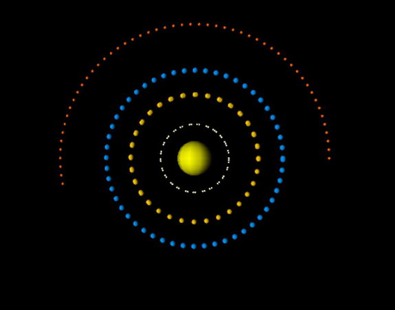
Figure 16-10. A basic solar system model that looks a bit artificial
This is a fully functional and physically quite realistic scale model of the solar system. Apart from the minor fact that the sizes of the planets and Sun are not visually represented in proportion to the distances between them, the real limitation of the model is that the initial conditions chosen for the planets are not actual instantaneous values; they are based on mean values of their distances from the Sun and their mean orbital velocities. Also, the planets are all aligned in a straight line to start with, which is a bit artificial. Let’s fix these limitations now.
Incorporating accurate initial conditions
We’re almost there, but to create a truly realistic solar system simulation you need to use accurate data as initial conditions. The only code that needs to change is really the setInitialConditions() method. You need to put some real data in there; you can get that data from NASA’s HORIZONS system here: http://ssd.jpl.nasa.gov/horizons.cgi.
This system generates highly accurate trajectory data (known as ephemerides) for a large number of objects in the solar system. The data is generated by NASA’s own simulation to extremely high accuracy (typically 16 significant figures!). You can choose the data type, coordinate origin, time span, and other settings. The file initial_conditions.txt, included with this example’s source code, contains some data that we downloaded for the positions and velocities of the eight planets at the time of 00:00 on 1 January 2012. Next to the name of each planet there are six fields that contain values of x, y, z, vx, vy, and vz, respectively. The positions are in km and the velocities in km/s, both relative to the Sun. We have used this data as initial conditions for the four planets we are simulating in the version of the code with the filename solar-system.js. Note that the setupPlanetData() method has also been simplified by removing the distances and velos arrays, which are no longer needed.
If you run the simulation you will find that the simulated trajectories now look more realistic with proper initial conditions (see Figure 16-11). Note in particular the characteristic eccentricity of Mercury’s orbit. Because we have access to NASA’s simulation data, why not compare our simulation with theirs?
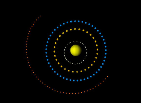
Figure 16-11. Planets’ trajectories in a 1-year simulation with our code
Comparing the model results with NASA data
We have also downloaded and saved position data from the HORIZONS web site for a whole year’s worth of simulation, from 1 Jan 2012 to 1 Jan 2013. The data is saved in CSV format in a separate file for each planet and is located in a subdirectory in the source code folder for this simulation. Note that the HORIZONS system is frequently updated as new measurement data is incorporated. The implication is that if you download data at a different time you may not obtain exactly the same figures to 16-digit accuracy. For most purposes, you wouldn’t even notice the difference, though!
To enable us to compare our simulation results with NASA’s data, we make a few small modifications to the previous code in solar-system.js. The new code is the file solar-system-nasa.js. The first change is to run the simulation for 366 days, by changing the value of numSteps to 8784. Next we change the value of animFreq to numSteps, so that the new planets’ positions are displayed only at the end of the 366 days. In the init() method just before rendering, we introduce a call to a new method, compareNASA(), which creates clones of the planets and places them at locations given by the NASA data on day 366. The remaining changes are in the simulate() method (see the bold lines in the following listing), with the replacement of the clonePlanet() method by a movePlanet() method, which moves the original planets to the new position instead of cloning them. Note also that the index i is replaced by i+1 in the if statement—this ensures that movePlanet() is not called initially (when i = 0) but on the last timestep.
function simulate(){
     for (var i=0; i<numSteps; i++){
          t += dt;
          for (var n=0; n<numPlanets; n++){
               RK4(n);
               if ((i+1)%animFreq==0){
                    movePlanet(n);
               }
          }
     }
}
function movePlanet(n){
     var planet = planets[n];
     planet.pos = s[n];
     positionObject(planet);
}
The result of these changes is that two copies of each planet are placed on the canvas on day 366 of the simulation. One set of planets is located based on the calculations of our simulation and the other set is located at the positions read from NASA’s data, each after exactly one year from the initial conditions. So how do they compare?
Run the simulation and you’ll see the planets in the locations shown in the screenshot in Figure 16-12. But why is there only one set of planets? The answer is that there are actually two sets—they are on top of each other! To convince yourself, add the following line of code just before the last line in the compareNASA() method:
p.pos = sN[i].multiply(2);
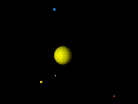
Figure 16-12. Planet positions after one year of simulated time compared with NASA data
What this does is to double the distance of each planet from the Sun for the cloned set of planets corresponding to the NASA data. Re-run the code and you will now find that there are indeed two sets of planets, one at double the distance from the Sun. So this shows that the NASA clones were on top of the original planets in the first run, and you just couldn’t distinguish between the two sets of planets at this resolution. Not bad, eh?
Although we have neglected a whole host of effects, such as the gas giants (especially Jupiter, the largest planet and the closest to the four terrestrial planets), asteroids, and relativistic effects, the results look pretty good. Of course, NASA’s simulation has all these and a lot more, together with much more advanced numerical methods, which make it much more accurate. It would be interesting to run the simulation longer or reduce the timestep to see at what point it starts to show visible differences compared with the NASA data. There are, of course, small differences, and bearing in mind that 1 px on the screen is a million km in reality, they may be significant in absolute terms. Nevertheless, while you may not necessarily be able to use this simulation to send your homemade space probe to Mars, you can most certainly use it to teach school kids or college students about how the solar system works.
Animating the solar system simulation
It is not difficult to modify the solar-system.js simulation to introduce some basic animation. This is done in the modified file solar-system-animated.js. First we replace the call to the simulate() method in init() by a call to the animFrame() method. We then introduce the following modified code, much of which should look very familiar:
function animFrame(){
     animId = requestAnimationFrame(animFrame);
     onTimer();
}
function onTimer(){
     if (nSteps < numSteps){
          simulate();
          moveCamera();
          renderer.render(scene, camera);
     }else{
          stop();
     }
     nSteps++;
}
function simulate(){
     t += dt;
     for (var n=0; n<numPlanets; n++){
          RK4(n);
          movePlanet(n);
     }
}
function movePlanet(n){
     var planet = planets[n];
     planet.pos = s[n];
     positionObject(planet);
}
function moveCamera(){
     camera.position.x += -0.1;
     camera.position.z += -0.5;
}
function stop(){
     cancelAnimationFrame(animId);
}
Note that the line that calls the renderer is now included in the time loop in onTimer(), so that the planets are re-rendered at their new location each timestep, producing the animation. We have also introduced a new moveCamera() method, which moves the camera as the animation progresses. Run the simulation to see the interesting visual effect this produces. You can experiment by making the camera move in different ways. For example, you can view the simulation from the perspective of a fixed Earth by replacing the two lines in moveCamera() with the following line:
camera.position.set(planets[2].position.x,planets[2].position.y,planets[2].position.z+200);
Figure 16-13 shows a screenshot of the resulting animation with this modification.
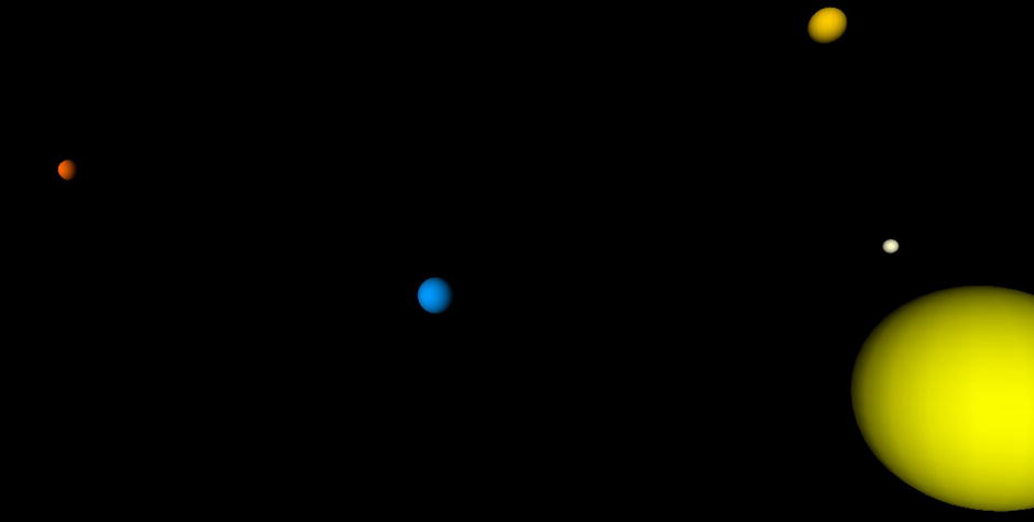
Figure 16-13. Animated version of the solar system simulation
It’s your turn
There are many ways in which you could develop or extend this simulation. The most obvious (and most straightforward) improvement would be to add in the four outer planets. You could also add in interactivity, dynamic scaling, enhanced animation effects, and so on.
There is also a whole host of 3D features waiting to be exploited here. Perhaps you can use actual image maps of the planets wrapped on them. Then you could add functionality to rotate and scale the view. Perhaps you could even show the planets spinning when they are close up. We’ll leave you to it.
Summary
With the completion of this book you now have a powerful set of tools at your disposal that will help you build more realistic and engaging games and animations as well as some pretty powerful simulations. From the simple bouncing ball simulation in Chapter 1, you’ve come a long way, indeed!
Let’s have a quick recap of all the ground covered in this book. In Part I, you went through a good deal of background material in JavaScript, math, and physics to establish the key concepts and techniques relating to physics-based motion and simulation.
Part II covered the basic laws of motion, and you encountered a wide variety of forces, building lots of examples that showed the interesting types of motion those forces produce.
In Part III, you simulated systems consisting of multiple particles or extended objects, including particle collisions, rigid bodies, and deformable bodies.
Finally, in Part IV you looked into how to create more complex simulations that require greater attention to numerical accuracy or that involve 3D or scale modeling.
That’s a lot of material.
This final chapter provided just a tiny glimpse of the possibilities that lie ahead for bringing all that physics together and putting it to use. We hope you will continue to have some serious fun with these projects as well as many others that you’ll build from scratch. We invite you to share your creations on the book’s website at www.physicscodes.com!